A comparison of methods that include estimation of spatial variation in the analysis of data from yield trials

!...

r-" " ~

A COMPARISON OF METHODS THAT INCLUDE ESTIMATION OF SPATIAL VARIATION IN THE ANALYSIS OF DATA FROM YIELD TRIALS

by

Cavell Brownie, Daryl T, Bowman, and Joe W. Burton

Institute of Statistics Mimeo Series No, 2236

September, 1992

MINEO Cavell Brownie, D SERIES Daryl_ T. Bm-Illlan and #2236 Joe W. Burton

:ri11;

A COMPARISON OF METHODS THAT INCLUDE ESTIMATION OF SPATIA

li

VARIATION IN THE ANALYSIS OF DATA

II

The library of the

Department of StMistics

\"\l

North Carolina State University

L.- -'

•

A Comparison of Methods that Include Estimation of Spatial

Variation in the Analysis of Data from Yield Trials.

Cavell Brownie,

Daryl T. Bowman*,

and

Joe W. Burton

Cavell Brownie, Dep. of Statistics, Box 8203, Daryl T. Bowman and Joe W. Burton, Crop

Science Dep., Box 7620, North Carolina State University, Raleigh, NC 27695. *Corresponding

author.

Abbreviations: CE, correlated errors; NN, nearest neighbor; RCBD, randomized complete

A Comparison of Methods that Include Estimation of Spatial

Variation in the Analysis of Data from Yield Trials.

ABSTRACT

In large yield trials, variation in soil fertility (or, more generally, yield potential) can result in

substantial heterogeneity within blocks, and hence in treatment estimates with poor precision.

Methods for improving precision include statistical analyses in which this spatial variation is

accounted for in the estimation of treatment or entry means. Three such types of "spatial"

analysis are reviewed; trend analysis, the Papadakis method, and analyses based on "correlated

errors" models which account for spatial variation through correlations between yields of

neighboring plots. Itis noted that, unlike the classical analyses which can be justified solely on the basis of the randomization employed in the experimental design, validity of these "spatial

analyses" in typical field situations is not guaranteed. Properties of these techniques are

discussed and the subjectivity involved in specifying a model for the spatial variation is

emphasized. Performance of the methodsis illustrated using data from two corn (Zea mays

L.) yield trials and a soybean (Glycine max L.) trial, each of which showed evidence of

heterogeneity within blocks. In comparison to the classical randomized blocks analysis,

precision tended to be best for the trend and the trend plus correlated errors analyses, with the

Papadakis method intermediate. Results for ranking of entries differ across analyses because

each analysis adjusts for spatial variation in a different way. Although using a spatial analysis

technique can improve precision, it can be difficult to determine which specific analysis is the

Many field trials in agriculture, including trials to determine genotypic yield potential, are

carried out using a complete block design. As is well known, the purpose of blocking is to

increase precision by ensuring that within a block treatments are evaluated with respect to

similar environmental (and operational) conditions. Heterogeneity among plots within a block

causes the estimate of a difference between two treatments to vary across blocks, and the

greater the heterogeneity within blocks, the greater the variation in estimates of treatment

effect and the poorer the precision of the study. Even with uniform cultivation practices, there

may be considerable variation in soil properties among plots in a block, and in general, the

larger the required block size, the greater is the within-block heterogeneity. Accordingly,

efficiency of the randomized complete block design (RCBD) tends to be poor in trials involving

a large number of treatments. To increase precision in such a trial, one approach is to reduce

block size by employing an incomplete block design such as a lattice, lattice square, or one of

the more flexible but potentially less efficient a-designs (Patterson et al., 1978). Another

approach is to use a method of analysis which utilizes information in plot position to estimate

and "correct for" spatial variation in yield potential due, for example, to differences among

plots in soil fertility, moisture, or even pest populations. These analyses require contiguous or

regularly spaced plots, arranged in a strip or rectangular grid, but given an appropriate layout

can be applied to data from a complete or incomplete block design.

Increasing efficiency via an analysis which includes estimation of spatial variation in

yield potential has been the focus of a number of recent articles in the agronomy and soil

science literature. Several methods have been described, including trend analysis (Kirk et al.,

1980; Tamura et al., 1988; Bowman, 1990), and the Papadakis method (e.g., Warren and

Mendez, 1982), also called nearest neighbor (NN) analysis (Bhatti et al., 1991), or Productivity

Covariate analysis (Longer and Risley, 1983). There is considerable confusion in terminology,

however, and the properties and relative merits of different methods (and the many variations

on each) are not well understood. Another potential source of confusion is that in promoting

solely on the basis of error mean squares calculated for a limited number of data sets.

Recommendations have beenbased on the assumption that the best method is that which produces the smallest calculated 'error', and there has been little attention given to validity of

estimates of precision or corresponding tests of hypothesis. In making comparisons with the

traditional randomized block analysis, there has also been a tendency to misrepresent the

properties of this analysis, especially properties that are a consequence of randomization which

is an integral part of the experimental design.

The goals of this article are therefore (i) to review the role of randomization in the

classical analysis, (ii) to describe the main types of analysis which include estimation of spatial

variation, and (iii) to provide a more balanced assessment of the properties of these methods,

including comparisons with the classical analyses. Illustrative examples are taken from corn

(Zea maysL.) and soybean (Glycine max L.) yield trials, and treatments are referred to as

entries throughout:

VALIDITY OF THE RCB ANALYSES

The assumptions usually listed for validity of the RCB analysis include independent and

identically distributed (iid) errors. Itis less frequently noted that the classical analysis can be

justified solely on the basis of the chance distribution induced by the design principle of

random assignment of entries to plots within blocks (Kempthorne, 1952). This property of the

RCBD is reviewed here because of a concern that promoting the use of procedures which

account for spatial variation could actually lead to suggestions that randomization is either

inappropriate or unnecessary when systematic heterogeneity is present.

The reason for randomization in experimental design is to provide unbiased estimates of

treatment effects or contrasts, and to provide valid estimates of residual variation or precision

(Steel and Torrie, 1980). When heterogeneity or even systematic trends are present within

blocks, assuming only additivity of entry effects, randomization ensures that, averaging over all

possible assignments or layouts, the difference between two entries is estimated without bias.

averaged over a large number of blocks.) Randomization also provides a framework in which

the traditional estimates of precision, and tests of hypothesis, are valid (Williams, 1986; Baird

and Mead, 1991). Thus 'biases' in treatment means reported by Tamura et al. (1988)

represent results for a single field layout and ignore the role of randomization in the RCBD

entirely. Also, contrary to statements in Bhatti et al. (1991), validity of the traditional

analysis does not require that 'soil ... properties exhibit random variability with little or no

spatial correlation.' Also incorrect are statements in Kirk et al. (1980) to the effect that

estimates of error and tests of significance for the "standard" analysis are biased. The presence

of undetected systematic variation within blocks does not invalidate the classical RCB

analysis, rather it strengthens the case for random allocation of treatments. On the other

hand, substantial heterogeneity within blocks results in estimates that are highly variable, so

that a nontraditional method of analysis might be considered in order to improve precision.

To motivate the nontraditional analyses, suppose that for a particular trial there is

considerable spatial heterogeneity in the site, and that the yield potential (e.g., fertility)

happens to be known for every plot. An efficient analysis would make use of these values and

accordingly adjust observed yields to obtain estimates of differences between entries. In

practice, plot yield potentials will, of course, be unknown but it seems reasonable to consider

the joint estimation of fertility trends and entry effects. To do this requires making

assumptions about the nature of spatial variation, and validity of the resulting "spatial"

analysis will depend on whether model assumptions are met or not. The problem is therefore

to compare two different types of analysis where each has a different basis for validity. The

physical process of randomization provides a basis for validity of the classical RCB analysis,

while the validity of analyses which estimate spatial variation depends on assumptions that are

impossible to verify for a single data set. To permit meaningful comparisons among analyses,

it is important, therefore, to investigate conditions under which the non-traditional analyses

yield valid tests of hypotheses and estimates of precision. Results of such investigations are

ANALYSES WITH ESTIMATION OF SPATIAL VARIATION

The analyses described below assume a rectangular axb layout of plots, with row

position indexed by Ri, i

=

_{1,...,a, and column position by Cj, j}

=

1,...,b. Each of the t entries is replicated r times, so that the total number of plots in the grid is ab

=

rt. For the plot in row i and column j, plot (ij), let Yij represent the observed yield, Tij the unknown yield

potential, and Tk(ij) the effect for the entry assigned to this plot. Then a model which

incorporates spatial variation is

Yij

=

J.C _{+ Tk(ij) + T ij + eij}

whereJ.C_{is an overall mean, Tk(ij) and T ij are assumed to be fIxed effects, and the eij are}

random errors with E(eij )

=

O.

As noted in Zimmerman and Harville, 1991, spatial variation can be incorporated in

this model at two levels. Major trends can be modelled as part of the mean through the T_ij

term, and small scale dependence can be included by allowing correlations between the plot

errors eij' The methods of analysis discussed below differ in the assumptions made about the

Tij and eij' The linear model for the RCB analysis is a special case of Eq. [1] with the

eij assumed iid and the value of Tij depending only on the complete block or replicatein

which plot (ij) is located.

Trend Analysis.

[1]

The term trend analysis has been used to describe an analysis based on the model in Eq.

[1] with the _{eij assumed to be iid, and T ij assumed to be a polynomial function of Ri and Cj}

(for more detail, see Kirk et al., 1980; Tamura et al., 1988; Bowman, 1990; or Warren and

Mendez, 1982, who use the term polynomial regression rather than trend analysis). As an

example, assume that yield potential can be represented by a 2nd degree polynomial response

surface (c.f. Zimmerman and Harville, 1991). Then trend analysis corresponds to fItting the

model in Eq. [1] with

the eij assumed iid, Var(eij)

=

(7"2, and

T ..

=

b_{iR. + b2C. +}

b3R~ +b4C~

+ bSR.C..

Note that block effects are not included in Eqs. [1] and [2] on which trend analysis is

based. This is because one of the arguments given for trend analysis is that boundaries

between contiguous blocks are artificial in the sense that yield potential is not likely to change

abruptly along straight lines corresponding to these boundaries. Including a term for blocks in

Eq. [1] or [2] would result in a model for yield potential with discontinuities along block

boundaries, whereas trend analysis assumes that yield potential varies in a smooth manner.

Under the model given by Eqs. [1] and [2], estimates of the entry means (corrected for

differences in yield potential between plots) and of the parameters b1, ... , bS' as well as tests

of significance, are easily obtained using PROC GLM in SAS (version 6.07; SAS Institute,

Cary, NC). Kirk et al. (1980) explain that fitting the polynomial response surface corresponds

to partitioning out of "error" the systematic component of heterogeneity, and estimates of

precision are based on the remaining random component only. Examples are given of the

increase in (calculated) precision achieved by reducing error in this way.

Although trend analysis can result in increased efficiency, potential shortcomings of this

approach should not be overlooked. These include problems associated with overfitting or

with using an incorrect model. Overfitting occursif_{the true function for T ij is a polynomial}

but we fit a polynomial with too many terms. Fitting an incorrect model occurs if too few

terms are fitted, or if the true function cannot be modeled as a polynomial. Overfitting tends

to add noise (rather than bias) to estimates of entry means, and can lead to poor performance

because of near confounding between polynomial terms and entry effects. Fitting an incorrect

model will result in biased estimates of entry effects and can lead to inflated (i.e., larger than

nominal) type I error rates. For data sets where strong trends are evident, however, numerical

studies suggest that the increase in precision will often more than compensate for bias which

results when the polynomial is at best an approximation (e.g., Zimmerman and Harville,

1991).

An important component of trend analysis, therefore, is deciding how to select the

Warren and Mendez, 1982, suggested an 8th degree polynomial, but did not assess validity of

estimates of precision or tests of significance. Another approach is to select the terms of the

polynomial by means of an algorithm analogous to procedures used for variable selection in

stepwise regression (Kirk et al., 1980; Tamura et al., 1988). This selection algorithm involves

performing a number of preliminary tests of significance to determine the terms to be included

in Tij. ABa consequence, p-values based on the final model are likely to be liberal (too small),

and estimates of precision are likely to be optimistic. In a limited numerical study, Tamura et

al. (1988, Table 3) indeed found inflated Type I error rates for the test for differences between

entries. To improve Type I error rate properties, Tamura et al. suggested that a significance

level of .01 be used in determining the polynomial terms to be included in Tij"

Variations on trend analysis therefore include different procedures for choosing the

polynomial for T ij. Other variations involve specifying functions other than polynomials based

e.g., on Fourier series expansions (Warren and Mendez, 1982). Problems associated with

specifying the degree of the polynomial function for T ij are also encountered with other types

of series approximation.

Papadakisanalysis.

Although it is difficult to describe a rigorous basis for this analysis (e.g., Kempton and

Howes, 1981), the Papadakis method has considerable intuitive appeal. A residual is

calculated for each plot by subtracting the appropriate entry mean from the plot yield. A

measure of yield potential, Xij' is then computed for each plot as the average of the residuals

for the neighboring plots. Adjusted means are obtained for entries by treating the measures

Xij as values of a covariate. That is, adjusted means for entries are based on fitting the model

Yij

=

JJ + Tk(ij) +bXij+eij

where, for interior plots,

Xij

=

1/4 (riJ-1 + riJ+1 + ri-1J +ri+1J)'

rij

=

Yij -

Y

k(ij)'

and

Y

k(ij) is the mean yield for the entry assigned to plot (iJ).

[3]

[4]

For border plots, Xij is the mean of the rij for the 2 or 3 neighboring plots.

As with trend analysis, blocks are ignored when carrying out the Papadakis analysis.

Again, this is because including block effects would introduce seemingly artificial

discontinuities in yield potential for plots that are adjacent but in different blocks. The

Papadakis analysis is sometimes described as an analysis of covariance, but note that X_ij is not

a true covariate because the rij are calculated from the observed yields Yij' Versions ofthe

Papadakis analysis are also referred to as nearest neighbor analyses (Bhatti et aI., 1991; Pearce

and Moore, 1976), however the term (nearest) neighbor analysis is also used in a generic way

to denote any analysis which utilizes information from neighboring plots in accounting for

spatial variation. The Papadakis analysis, including calculation of adjusted entry means, can

readily beimplemented using SAS (see Appendix).

Variations on the Papadakis method include using different subsets of residuals to

compute Xij' For example, Xij may becomputed from residuals of neighbors in the same row

only [Xij

=

1/2 (riJ-1 + riJ+1)]' Also, more than one "covariate" may befitted, so that Eq. [3] may contain one "covariate" for residuals in the same row and a second for residuals in the

same column (e. g., Zimmerman and Harville, 1991). Yet another variation is the iterated

Papadakis method (e. g., Bartlett, 1978) in which Eq. [3] represents step 1, and the adjusted

means from Eq. [3] areusedto calculate step 2 residuals rfl) and yield potentials Xh2). Step 2

adjusted means are then obtained by fitting the model in Eq. [3] with Xij replaced by xh2).

The process isrepeated until adjusted means from consecutive steps are approximately the

same.

Properties of the Papadakis analysis are difficult to determine theoretically. Several

numerical studies (e.g., BinDS and Jui, 1985) of the performance of the method have concluded

that the uniterated version lacks efficiency, while the iterated method produces tests with

inflated Type I error rates. The inefficiency of the uniterated versionisattributed, in part, to

the fact that plot yield potentials and entry effects are not estimated jointly. Studies

Moore, 1976; Longer and Risley, 1983) have confIrmed that no single version will be best for

all fIelds or patterns of soil heterogeneity. Selecting the best "covariate(s)" for a particular

data set leads to problems analogous to those associated with choosing the polynomial

function in trend analysis.

Modelswit.hcorrelated errors.

The most recently developed methods of analysis are based on models that account for

small scale variation in soil properties through correlations between the plot errors fij.

Typically, these models assume that the strength of the correlation between two errors,

Corr (fij' flm)' is greatest for adjacent plots, and diminishes as the distance between the plots

increases. These models and corresponding analyses are more complex to describe and

implement than are either trend analysis or the Papadakis method. Most of the proposed

models are included in the general formulation given by Zimmerman and Harville (1991), but

only methods that are easily implemented with SAS are considered here. For example,

Zimmerman and Harville (1991) studied a modifIcation of the model in Eq. [1] where T ij is a

second degree polynomial and the correlation between plots decays exponentially as the

distance between the plots (or plot centers) increases. SpecifIcally, this model is given by Eqs.

[1]

and

[2],

with

2 ( ) 2 -8d(iJ· 1m) Cov(fij' Elm)

=

(1' Corr Eij' Elm

=

(1' e ' ,

where d(ij,lm)

=

the distance between (the centers of) plots (ij) and (I,m).

[6]

Variations on this model include specifying other polynomial functions for T ij and/or

alternative covariance structures for the errors Eij. The latter include I-dimensional correlation

structures, for example serial correlations between plots within the same row only. This

approach models large scale spatial trends through "fIxed-effect" polynomial terms for the

mean, as does trend analysis, but italsoallows for small scale dependence through correlations between neighboring plots. This"correlated errors" modifIcation of trend analysis is thus

opportunity for subjectivity to enter the analysis. Ifthe polynomial function for the trend and the covariance function have both been specified, the new PROC MIXED in SAS can be used

to carry out an appropriate analysis (see Appendix).

In theory, inferences provided by this "trend plus correlated errors" (trend+CE) analysis

are valid if the assumptions of Eqs. [1], [2] and [6] are correct for an appropriate target

population. In practice, it will be difficult to determine if these assumptions are even

approximately correct for a given data set, and properties of the analysis when the trend+CE

model is incorrect are not easily derived analytically. Accordingly, Zimmerman and Harville

carried out a numerical study using uniformity trial data to assess performance of the analysis

based on Eqs. [1], [2] and [6]. They found that this trend+CE analysis was more efficient than

an uniterated Papadakis analysis, and considerably more efficient than the RCB analysis.

The trend+CE analysis was also more efficient than the corresponding trend analysis with iid

errors.

To assess validity of each method, Zimmerman and Harville compared the averages

(over different randomizations or layouts) of two measures of precision: one based on the

predicted variance for that model, and the other an empirical estimate possible because of the

absence of treatment effects in uniformity trials. Results suggested that estimates of precision

basedon the trend+CE model generally agreed well with the empirical estimates. In

comparison, estimates of error produced by both the Papadakis and trend analyses were found

to differ considerably from the empirical estimates, the Papadakis estimates being consistently

pessimistic. As expected, validity of the RCB analysis was demonstrated, even though

systematic heterogeneity was evident in the uniformity trial yields.

Zimmerman and Harville (1991) caution that the favorable results for the model with

covariance as in Eq. [6] (and for related models with asymmetric correlation structures) are

preliminary, beingbased on 3 data sets each with a limited number of plots. They also note that there is no simple solution to the problem of how to select an appropriate covariance

Zimmerman and Harville are sufficiently promising, however, to warrant further investigation

of analysesbased on models with correlated errors to account for spatial variation in data from

large yield trials.

EXAMPLES

Properties of the analyses described above are illustrated using data from two corn yield

trials (Bowman, 1985) and a soybean trial. Each corn trial included 30 commercial entries, the

experimental design being a 6x5 rectangular lattice in 3 replicates (c.f., Cochran and Cox,

1957), laid out with the 18 incomplete 5-plot blocks arranged in an 18x5 grid (see Fig. 1). The

soybean trial contained 180 inbred lines or entries in 3 replicates, with entries in 10 sets of 18

in a split plot type of arrangement (c.f., Cochran and Cox, 1957, p. 388). Each complete block

or replicate was 70m

x

35m in area, with plots arranged in a 15

x

12 grid. However replicates

were not contiguous, being separated by alleys. More detail isgiven for the corn trials than for

the soybean trial partly because the corn trials allow comparisons with incomplete block

designs and partly because presentation of results is easier with 30 than with 180 entries.

Corntrials 1and 2.

To examine the data from each trial for systematic trends in yield potential, residuals

rij were calculated as in Eq. [5] and plotted against row position R_iand, separately, against

column position C_j. The following series of analyses was then applied to the data from each

trial:

(a) the RCB analysis,

(b) the lattice analysis with incomplete block effects assumed random,

(c) a Papadakis analysis with a single "covariate" as in Eqs. [3] and [4],

(d) trend analysis with the polynomial function for Tij selected using the Tamura et al.

(1988) modification of a program developed by Kirk et al. (1980),

(e) trend+CE, a correlated errors modification of (d) with the polynomial for Tij as in

(d), and Corr(lij' lIm) as in Eq. [6], and

replicates and Corr(fij' flm) as in Eq. [6].

SAS code for carrying out each of these analyses is given in the Appendix.

Comparing results for these different analyses is not a straightforward matter. This is

because for a given trial, the true ranking of entries and the actual pattern of spatial

heterogeneity are both unknown. Conceptually, there are also difficulties relating to the

implied target populations if block effects are assumed random in the traditional analyses. In

fact, there is no completely objective way to determine which analysis is the most appropriate

for a single data set. Nevertheless, it is informative to compare certain results from these

analyses, keeping in mind what is known about the properties of each.

Ideally, comparisons of precision among analyses should be based on the variances or

standard errors of estimated entry effects or contrasts. For each data set and analysis, a model

basedestimate of the standard error can be calculated for each adjusted entry mean. The

average of these standard errors then provides a measure of precision for comparing analyses

(Table 1). Other articles (e.g., Warren and Mendez, 1980; Kirk et al., 1982; Tamura et al.,

1988) have based comparisons of precision on the error mean square. This is reasonable for the

RCB, trend and Papadakis analyses since the standard error of an adjusted entry mean is

largely determined by the (square root) of the error mean square. For the CE models,

however, because of the more complex variance structure, precision cannot be summarized

using a single mean square analogous to the error mean square. Accordingly, the root error

mean square is reported in Table 1 for the RCB, trend and Papadakis analyses, but there is no

corresponding entry for CE and trend+CE analyses. For the lattice analysis, precision depends

on whether incomplete blocks are assumed random or fixed, the latter being more closely

analogous to the fixed effects model of trend analysis. Itwas decided to perform the lattice

analyses with incomplete blocks random, but the square root of intrablock error is given in

Table 1 as an indication of precision of the lattice analysis with fixed block effects.

To further examine differences between analyses, comparisons were also made of the

means were compared across analyses to illustrate that the different methods of accounting for

spatial variation can lead to quite different results with respect to ranking of entries. This

seems important to emphasize because it will usually be impossible to determine which analysis

produces the most accurate ranking of entries for a given trial.

Plots of residuals, corrected for entry effects only (see Eq. [5]), against row position

showed evidence of systematic trends in yield potential for both trials (Fig. 2). Plotting

residuals against column position was less informative. The model selection procedure in

Tamura et al. (1988) on the whole supported this visual assessment resulting in a 4th degree

polynomial on row position for trial 1, and a polynomial involving both row and column terms

for trial 2. Consequently, substantial reductions in "unexplained variation" can be achieved by

a nontraditional analysis, and average standard errors are largest for the RCB analysis which

accounts for spatial heterogeneity only through differences between the 3 complete replicates

(Table 1). For trial 1 where the rows correspond to incomplete blocks, and trend appears to

depend mainly on row position, the lattice analysis is effective. For trial 2, where yield

potential seems to depend to some extent on both row and column position, the lattice analysis

is comparatively less effective. Accordingly, trend analysis produces an increase in precision

comparable to that for the lattice in trial 1, but appears more efficient than the latticein trial 2. The Papadakis analysis is intermediate between the RCB and trend analyses in both eases.

Several correlated errors models were fit to the data and only the most noteworthy

results are reported. When the polynomial terms specified for Tij were selected as in Tamura

et al. (1988), there was little difference between results obtained with trend analysis (i.e.,

assuming the fij iid) and the corresponding correlated errors (or trend+CE) analysis. This was

true whether the correlation structure was assumed to be 2-dimensional as in Eq. [6] or

1-dimensional either within rows or within columns. On the other hand, accounting for spatial

variation using a correlated errors structure but no trend other than replicate effects (CE

analysis) did not appear to improve precision relative to the RCB analysis.

lattice, and trend analyses, these estimates depend on row position only, while the Papadakis

estimates are different for each plot. For comparison, the average of the Papadakis Xij values

for each row is plotted with the other 3 estimates. For the RCB analysis, yield potential is

assumed to be the same for the 6 rows in each complete block, and the estimated trend is thus

a step function. In contrast, the lattice and trend analyses suggest systematic variation within

blocks 1 and 3, with yield potential tending to increase with row position. Comparing the

lattice and trend estimates, the lattice estimates agree closely with the row averages of the

residuals (not shown) resulting in a rough pattern in Fig. 3a, while the trend estimates are like

a smoothed version of these points (corresponding approximately to fitting a 4th degree

polynomial to the lattice estimates).

For trial 2, the surface estimated by trend analysis has gradients in both row and

column directions, whereas the lattice estimates are necessarily constant within each row. As a

consequence, estimates of yield potential from these analyses agree reasonably well in the

center plot of each row (Fig. 3c) but agree less well for the extreme plots in each row (i.e., for

plots in colums 1 and 5, Figs. 3b and 3d respectively). Like the trend analysis estimates, the

Papadakis estimates of yield potential are different for each plot, but the Papadakis estimates

are not obviously closer to the trend estimates than to the lattice estimates.

The test for entries was not significant for trial 1, but adjusted means are presented for

both trials in Table 2, as both sets of means illustrate how results can differ according to the

analysis used. Note that the greater differences among analyses in estimates of spatial variation

for trial 2 are reflected in larger differences in adjusted means across analyses for trial 2 than

for trial 1 (see Table 2). Also in both trials it is evident that estimated entry means for the

analyses that adjust for spatial variation differ substantially from the estimates for the RCB

analysis. Comparing the trend and lattice analyses for trial 1, the largest differences between

adjusted means are for entries 27 and 28, with entry 27 ranked 3rd by the lattice analysis and

only 11th by trend analysis. Both of these entries occur in rows for which the trend estimates

lower for the trend than for the lattice analysis.

For trial 2, analyses differ considerably with respect to entry 10, which is the top

ranking entry for the Papadakis and trend analyses, but is 4th for the lattice analysis. Entry

10 occured in two plots for which yield potential was estimated to be low under the trend

analysis, and accordingly was adjusted upward relative to the other entries, giving a yield of

11807 kg ha-1 for trend analysis, compared to 10799 kg ha-1 for the lattice analysis.

Although less important for interpretation of results, there was also a large difference in the

estimated means for entry 25 in the different analyses (Table 2). Like entry 10, entry 25 was

located in plots with low estimated yield potential under the trend analysis.

Soybean trial.

Residuals obtained after fitting entry effects only, when plotted against column position

showed evidence of trends from left to right within each replicate (Fig. 4). Effects of row

position were more-difficult to elucidate from plots.

Yield was missing for two of the 540 plots in this large trial, and so the RCB analysis

was modified by computing adjusted means for entries. Analyses which estimate spatial

variation required no modification because of the missing plots, but did have to be modified

slightly because replicates were not contiguous. The Papadakis analysis was implemented by

calculating the "covariate" values Xij as in Eq. [4] but using residuals from plots in the same

replicate only. The Tamura et a!. (1988) program could not be used to select the polynomial

model for trend analysis because replicates were not contiguous, and also because the number

of entries exceeded 50. Instead, basedon the residual plots, PROC GLM was used to fit a

polynomial within each replicate which included all first and second order terms plus cubic and

quartic terms for rows. This model was then simplified by successively eliminating the highest

order nonsignificant (p>.Ol, Tamura et al., 1988) terms. Two trend+CE analyses were carried

out, trend(l)+CE using the polynomial row and column terms exactly as in trend analysis,

and trend(2)+CE with only a linear column effect within each replicate. A I-dimensional

2-dimensional structure in Eq. [6], and was implemented with both trend(I)+CE and

trend(2)+CE.

Evidence of spatial heterogeneity was reflected in the highly significant "covariate" in

the Papadakis analysis, and also in highly significant row and column polynomial effects.

Average standard errors were similar for the Papadakis, trend, and trend+CE analyses, and

about 20% smaller than for the RCB analysis (Table 3). Correspondingly, the root error mean

square for the Papadakis and trend analyses was about 80% that for the RCB analysis. The

similarity between standard errors for the two trend+CE analyses suggests that, as noted by

Zimmerman and Harville (1991), the correlation structure can to some extent 'absorb' large

scale trend not accounted for in Tij"

Comparing analyses in terms of estimated entry means, agreement tends to be greater

among the trend and trend+CE analyses than between any of these and the RCB analysis

(Figs. 5a, 5b). Comparing results for the top ranked entries, 11 entries were ranked in the top

20 by all five methods, and six of these were ranked in the top 10 by all methods.

DISCUSSION AND CONCLUSIONS

For each of the examples presented it is evident from plots of residuals that there were

trends in yield potential which resulted in heterogeneity within complete blocks. For field

sites like these, there is disagreement on whether to improve precision by using an incomplete

block design or by using an analysis which accounts for (within block) spatial variation.

Reasons for not using incomplete block designs such as the lattice or lattice square relate to the

practical difficulties imposed by restrictions on the number of entries that can beincluded and the inconvenience incurred when a decision is made to include additional entries after field

plans have been prepared. The main argumentagai.ostusing a nontraditional spatial analysis

is that properties of these analyses for typical field situations are largely unknown, whereas a

simple randomization argument provides validity for the traditional RCB and intrablock

lattice analyses. The reason for using a nontraditional spatial analysis is that greater gains in

design and the conventional analysis.

On the basis of examples discussed here (see also Kirk et aI., 1980; Pearce and Moore,

1976; Bowman, 1990, etc.) and numerical studies in Zimmerman and Harville (1991), Baird

and Mead (1991), Binns and Jui (1985), it seems clear that precision can be improved by using

a nontraditional analysis without necessarily sacrificing validity. An example where the

lattice design and analysis are ineffective and a spatial analysis is more efficient is provided by

the second of the corn trials where gradients in yield potential are not I-directional. Note,

however, that this is not an argument against use of incomplete block designs, because a

spatial analysis can be applied to data obtained with such designs.

Perhaps more difficult than deciding whether to use a nontraditional analysis, is the

problem of selecting a particular spatial model and analysis. The examples given here

illustrate clearly that Papadakis, trend, and correlated errors analyses will produce different

rankings of entries" for a given data set. Results will also depend on how the Papadakis

"covariate" is calculated, on the polynomial used to model trend, and on the covariance

structure assumed. No simple rules can be given for deciding which is the best analysis,

instead some of the issues to be kept in mind are noted below.

In simple regression problems such as relating yield to rate of fertilizer applied,

polynomials can be useful approximations to the true relationship. On the other hand,

polynomials can be entirely inappropriate as when the response curve plateaus. Similarly,

polynomials will not always be good approximations to the variation in yield potential in a

field, and the presence of entry or variety effects in the data makes it harder to detect poor fit

than in a simple regression problem. Approximating trend using a polynomial can increase

precision without introducing substantial bias, but for a given trial results for one or more

entries could be misleading if the yield potential surfaceisnot well approximated by a polynomial model.

The Papadakis analysis will not be as efficient as trend or trend+CE analyses when an

relies less on a specific shape for the yield surface it will be less likely than trend analysis to

produce adjustments to means that are extreme. This is apparent in both the soybean and

second corn trial, where the Papadakis adjustments are on average substantially (about 40%)

smaller than for trend and trend+CE analyses. Comparing the Papadakis and trend analyses,

there is the usual trade-off between possible gains in efficiency versus increased bias incurred by

making more stringent assumptions about the data (specifically, about the form of the yield

surface).

Zimmerman and Harville (1991) and Baird and Mead (1991) claim that the best gains

in precision overall are made with correlated errors models, and for the soybean trial the

trend+CE analyses did seem to be effective. For the corn trials examined here, however, there

seemed to be little to be gained by assuming errors correlated in comparison to trend analysis

as implemented using the Tamura et al. (1988) program.

Considerable detail has been omitted in this review of spatial analysis techniques useful

for yield trials. In particular, correlated errors models have received very brief treatment. A

topic that has been ignored entirely is that of designs developed specifically for use with spatial

analyses (see, e.g., Williams, 1985). Also the use of spatial analyses when the goal is to

combine results from a series of trials over space and time has not been addressed here or

elsewhere. Objective methods to assist in selecting the best analysis for a particular data set

have not been developed but are clearly needed. Itis hoped that by providing SAS code,

researchers will be encouraged to implement several of these analyses and thus provide

empirical information on their performance. Careful evaluation of the results by a number of

researchers should then lead to better understanding of the methods and their advantages and

REFERENCES

Baird, D. and R. Mead. 1991. The empirical efficiency and validity of two neighbour models.

Biom. 47:1473-1487.

Bartlett, M. S. 1978. Nearest neighbour models in the analysis of field experiments. J. R.

Stat. Soc., Ser. B 40:147-174.

Bhatti, A. U., D. J. Mulla, F. E. Koehler, and A. H. Gurmani. 1991. Identifying and

removing spatial correlation from yield experiments. Soil Sci. Soc. Am. J. 55:1523-1528.

Binns, M. R., and P. Y. Jui. 1985. A simulation study of the nearest neighbour analysis

method of Papadakis. Comm. Stat. - Simul. Compo 14:159-172.

Bowman, D. T. 1985. Measured crop performance. I. Corn hybrids. North Carolina State

Univ. Res. Rep. 102.

Bowman, D. T. 1990. Trend analysis to improve efficiency of agronomic trials in flue-cured

tobacco. Agron. J. 82:499-501.

Cochran, W. G., and G. M. Cox. 1957. Experimental designs. John Wiley& Sons, New York.

Kempthorne, O. 1952. The design and analysis of experiments. John Wiley &Sons, New York.

Kempton, R. A., and C. W. Howes. 1981. The use of neighbouring plot values in the analysis

of variety trials. AppI. Stat. 30:59-70.

Kirk, H. J., F. L. Haynes, and R. J. Monroe. 1980. Application oftrend analysis to horticultural field trials. J. Am. Soc. Hort. Sci. 105:189-193.

Longer, D. E., and M. A. Risley. 1983. Improved precision in soybean variety trials. Proc.

13th Soybean Res. Conf. p. 22-28.

Patterson, H. D., E. R. Williams, and E. A. Hunter. 1978. Block designs for variety trials. J.

Agric. Sci. 90:395-400.

Pearce, S. C., and C. S. Moore. 1976. Reduction of experimental error in perennial crops,

Tamura, R. N., L. A. Nelson, and G. C. Naderman. 1988. An investigation of the validity

and usefulness of trend analysis for field plot data. Agron. J. 80:712-718.

Warren, J. A., and I. Mendez. 1982. Methods of estimating background variation in field

experiments. Agron. J. 74:1004-1009.

Williams, E. R. 1985. A criterion for the construction of optimal neighbour designs. J. R.

Stat. Soc. B 47:489-497.

Williams, E. R. 1986. Neighbour analysis of uniformity data. Aust.J. Stat. 28:182-191.

Zimmerman, D. L., and D. A. Harville. 1991. A random field approach to the analysis of

APPENDIX

The SAS (version 6.07) code included here was used to carry out the analysis of the corn trial data. The calculation of row and column positions (R, C) from plot numbers is specifically for plots in an 18x5 grid, and numbered in serpentine fashion, as indicated in Fig. 1. Note, however, that the PROC TREND code used to obtain the 4th degree polynomial for trend analysisisnot included.

/. SPATIAL.SAS./

••••••calculate row and column positions from plot number•••••; DATA SUB; SET 'inputfile';

IF LOC=3;

ROW=INT«PLOT-l)/5) +1; COL=MOD«PLOT-l),5) +1;

IF MOD(ROW,2)=0 THEN COL=6-COL;

KEEP LOC ROW COL YIELD ENT REP PLOT; ••••••calculate papadakis covariate••••••;

PROC SORT; BY ROW COL;

~PROC GLMj CLASS ENTj

MODEL YIELD=ENTj

OUTPUT OUT=NEW R=RESj DATA LEFTj SET NEWj

COL=COL+lj IF COL <=5j LEFT=RESj

KEEP LOC LEFT COL ROW; DATA RIGHT;SET NEW;

IF COL >=1;

RIGHT=RES;

KEEP LaC RIGHT COL ROW;

DATA TOP; SET NEW;

ROW=ROW-1;

IF ROW >=1;

TOP =RES;

KEEP LaC TOP COL ROW;

DATA BaTT; SET NEW;

ROW=ROW+1;

IF ROW <=18;

BOTT=RES;

KEEP LaC BaTT COL ROW;

DATA TOG; MERGE SUB LEFT RIGHT TOP BaTT; BY LaC ROW COL;

COV=MEAN(LEFT,RIGHT,TOP,BOTT);

PROC PRINT;

TITLE 'PAPADAKIS ANALYSIS';

PROC GLM; CLASS ENT;

MODEL YIELD=ENT COY;

LSMEANS ENT/OUT=PAPAD;

DATA A; SET SUB;

******calculate orthogonal polynomial contrasts for trend analysis;

R1=ROW-9.5; R2=RhR1 - 323/12;

R3=RhR2-64*R1/3; R4=RhR3- 8hR2/4;

PROC GLM DATA=A; CLASS REP ENT;

LSMEANS ENT/ OUT=RCBDj

TITLE 'RCB ANALYSIS'j

PROC GLM DATA=Aj CLASS ENTj

MODEL YIELD=ENT Rl R2 R3 R4j

LSMEANS ENT/OUT=TRENDj

TITLE 'TREND ANALYSIS'j

PROC MIXED DATA=Aj CLASS REP ENT ROW COL PLOTj

MODEL YIELD=REP ENTj

REPEATED PLOT/TYPE=SP(POW)(ROW COL) SUB=REPj

LSMEANS ENTj

MAKE 'LSMeans' OUT=CEj

TITLE 'CE ANALYSIS'j

PROC MIXED DATA=Aj CLASS REP ENT ROW COL PLOTj

MODEL YIELD=ENT Rl R2 R3 R4j

REPEATED PLOT/TYPE=SP(POW)(ROW COL) SUB=REPj

LSMEANS ENTj

MAKE 'LSMeans' OUT=TRENDCEj

TITLE 'TREND+CE ANALYSIS';

PROC MIXED DATA=Aj CLASS REP ENT ROW PLOTj

MODEL YIELD=REP ENTj

RANDOM ROW/ SUB=REPj

LSMEANS ENTj

MAKE 'LSMeans' OUT=LATTICEj

TITLE 'LATTICE ANALYSIS'j

DATA Bj SET RCBDj RCBDMN=LSMEANj

DATA Cj SET TRENDj TRENDMN=LSMEANj TRENDSE=STDERRj

DROPLSMEANSTDER~

DATA Dj SET TRENDCE; TRCEMN=LSMEAN; TRCESE=SEj DROP LSMEAN SE DF T P_ T LEVELj

DATA E; SET CEj CEMN=LSMEAN; CESE=SEj DROP LSMEAN SE DF T P_ T LEVEL;

DATA F; SET LATTICE; LATTMN=LSMEAN; LATTSE=SE; DROP LSMEAN SE DF T P_ T LEVELj

DATA G; SET PAPADj PAPADMN=LSMEANj

PAPADSE=STDERR; DROP LSMEAN STDERR; DATA MEANTOG; MERGE B G F C D E; DROP _NAME_; PROC PRINT;

Table 1. Square root of the calculated error mean square (REMS), average standard error of

an entry mean (AVSE), error degrees of freedom (edf), and F ratio for the test of no entry

effects, for six different analyses of data from two corn yield trials.

Trial 1 Trial 2

Analysis REMS AVSE edf F REMS AVSE edf F

kgha-1 kgha-1

RCBD 981 566 58 1.21 852 492 58 3.59

Lattice 772t 508

43t

1.34 813t 490

43t

3.54

Papadakis 863 501

59t

1.04 786 454

59t

3.90

Trend 808 475 56 1.39 599 362 53 7.05

Trend+CE -§ 470

56t

1.34 -§ 370

53t

7.07

CE -§ 544

58t

1.25 -§ 505

58t

5.81

t intrablock error.

t

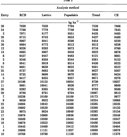
error or 'denominator' df, and F test, are approximate.

Table 2. Estimated yields for 30 commercial entries from five different analyses of the data from two corn trials. Entries are ranked according to the estimate from trend analysis.

Trial 1 Analysis method

Entry RCB Lattice Papadakis Trend CE

--- kg ha-1 _________________________________________

Table 2 continued.

Trial 2 Analysis method

Entry RCB Lattice Papadakis Trend CE ________________________________________ kg ha-1 ---_______________________________ 26 7839 7838 7794 7520 7866 24 7700 7778 7748 7846 7645 3 7971 8177 8551 8435 8405 28 8715 8743 8653 8437 8400 15 8907 8841 8596 8454 8320 20 8864 8773 8512 8512 8326 12 9326 9293 9073 8716 8760 13 8865 8907 8859 8822 8676 6 9427 9447 9483 9121 9091 2 9346 9358 9244 9261 9152 8 8841 8919 9314 9438 9323 21 9661 9639 9622 9501 9522 25 8737 8662 9106 9627 9307 14 9725 9699 9678 9631 9424 5 9417 9355 9257 9671 9278 27 10196 10153 10054 9730 10037 11 9991 10041 9826 9777 9689 30 9292 9365 9735 9782 9580 29 9789 9791 9704 10067 9813 7 10226 10169 10109 10172 9977 9 9850 9922 10269 10254 10068 22 10894 10842 10486 10385 10525 18 10602 10529 10368 10388 10132 23 9975 9834 10049 10392 10154 17 10976 10968 10636 10393 10549 19 10589 10599 10444 10448 10347 16 10679 10552 10802 10486 10440 1 10443 10469 10412 10530 10404 4 10980 11131 11057 10989 10876

Table 3. Square root of the calculated error mean square (REMS), average standard error of

an entry mean (AVSE), error degrees of freedom (edf), and F ratio for the test of no entry

effects, for 5 different analyses of yields from a soybean trial involving 180 inbred lines or

entries.

Analysis REMS AVSE edf F

RCBD Papadakis

Trend Trend+CE (1) Trend+CE (2)

---kgha-1

---633 366 497 288

504 298 - tt 278

- tt

284

356 357t 345 345t 353t

3.29

5.12

4.54 5.43 5.27

t

error or 'denominator' df and F test are approximate.

FIGURE CAPTIONS

Fig. 1. Field layout for corn trial 1, showing allocation of the 30 entries to plots which are

numbered in serpentine fashion and arrayed in an 18x5 grid. The design is a 6x5 rectangular

lattice, with six incomplete blocks (Rows) in each of three complete replicates (Reps).

Fig. 2. Residuals (plot yield - mean for entry) plotted against row position and identified by

column position, (a) for corn trial 1, and (b) for corn trial 2.

Fig. 3. Estimated plot yield potentials (kg ha-1) for RCB analysis (*), lattice analysis (A),

Papadakis analysis(0), and trend analysis(+), plotted against row position. Estimates in (a) are for corn trial 1 and (0) represents the average of the Papadakis estimates for a row.

Estimates in (b), (c), and (d), are for plots in columns 1, 3, and 5, respectively, for corn trial 2.

The RCB (*) and lattice (A) estimates depend on row position only and are the same in (b),

(c), and (d).

Fig. 4. Residuals (yield - mean for entry) for soybean trial plotted against column position.

The basic-design was an RCBD with 180 entries in three replicates. Each replicate was a

15x12 grid of plots, but replicates were not contiguous in the field, being separated by alleys

running between columns 12 and 13 and between columns 24 and 25.

Fig. 5. Agreement between adjusted entry means for three of the five analyses applied to the

RepIII

Rep II

Rep I

90 89 88 81 86

?7 1~ 7 10 %

81 82 83 84 85

11\ 1> 23 ?Q 14

80 79 78 71 76

1? 1\ 1R ?.:1 .:1

71 72 73 74 75

~n ?1 1 R ?n

70 69 68 67 66

?I\ ?? ? 11> 0

61 62 63 64 65

10 3 11 ?R 17

60 59 58 51 56

?.:1 R ?Q 3 13

51 52 53 54 55

? 7 ?~ 1R ?R

50 49 48 47 46

.:1 Q 30 14 1Q

41 42 43 44 45

_ ?O fi 1fi 10 2fi

40 39 38 31 36

1\ ')1 ')1\ 11 11\

31 32 33 34 35

17 1 1') ?7 ??

30 29 28 21 26

?~ ?1> ').:1 ?1 ??

21 22 23 24 25

R 1\ 7 10 Q

20 19 18 11 16

?I\ ?7 30 ?Q ?R

11 12 13 14 15

1 1> 4 ~ ?

10 9 8 1 6

11> 11 14 1~ 1?

1 2 3 4 5

1R 11\ ?O 17 1Q

18

12

6

1

Row

(a)

(b)

3000

""

3000

Ol

i.

1000

(1j

r

2000

1

1

1 4

5

3 2

3

5

8

5 5

H

4

3

3

d

3 4

4 3

4

01 3

5

5

1.

~

8

f

1 2 1

2

41

21$

5

2

5 2

~

2

1

j

22

3

2

34

4

3 4 3

22

~

4

q

1

T

5

1

1

2000

1000

-1000

-2000

4

4

2 3

5

5

5 4

3 d 3

4

435~

a

2 1 3

4

3 4

22

4

1

OJ

1

2

~

5

1

5

1 5

4

2

a

4 3

!

T

3 13

I

12

32

1

5

l '

d

113

3 1

4

2

g

4

~

4

5 5 1

§

v

(1j

::J

-1000

'0

"

.

-1

4

6

8

10

12

14

16

18

Row

2 4 6

8

10

12

14

16

18

,.

( a )

2000

-

as

.c 1250

-

Cl A

~

-

500

A

( b )

A

* * otl * • ~

o

1250 A O -250 500

2 0 0 0 . . . - - - ,

-1000 -1750

...

A,ri

0 I

rtJ

A I **Q'*** A

,

f

,

,r...,{')

Ci A

, 0 ' 1 ( . :;

(. A',~ ,

I 0 \ A , '

*

*/0 * * *

o'~

6

/J

l:I' A

* ...

't, •

0 ...

5

cp

A "t---l"

,

of

,

,

,

AI

,,

I

,

+

as

CD -1750 ... -250 c: CD

>-o

a.

-1000

...

8 1 0 1 2 1 4 1 6 1 8

6 4

2

- 2 5 0 01---.r__--r--.--..__----.---r--.---...---.,...J

o

8 1 0 1 2 1 4 1 6 1 8

6 4

2

- 2 5 0 0 ~-,....-___.-___r-...-_,_-.._____,r_____"T-~

o

( C )

( d )

.... -250

C

CD

....

o

a.. -1 000

2 0 0 0 . . . . - - - ,

1250

500

2 0 0 0 . , - - - ,

-250 -1000 500 1250

as

as

.c

-A

CD -1750 -1750

>-8 1 0 1 2 1 4 1 6 1 >-8

6

4 2

- 2 5 0 0

1---..---.--,..-_,_-.,..--..--___.-___"T---.--o

8 1 0 1 2 1 4 1 6 1 8

6

4 2

- 2 5 0 0 ~-,....-___.-___r-...-_,_-.._____,r_____"T-~

•

2500

2000

1500

+

+

+

++

+

+ +

•

o

4

8

1 2

1 6

20

Column

( a)

( b)

46001

+

4600

+

+

+

;}*+

-II

+

i

t+

'0

g~t

+

f'

~#*t+

H~.Jflt

-

Q)

.- 3600

3600

~

+It H

~

+f+

1#

itt

+++

'0

+J1

-' t

++}t

++

+"

(JJ

+

If

Q)

V~+*

+

t~

filt+

W

2600

,\t+t +

2600

+lit

+

/'IJI

0

+

itt

++

+

+

t-

+

t+

1""\

++t

*

+

C

t

+

+tt

++

'0

+

~

1600

+

1600

+

~

I

t

_;1

I

+

+

+

4600

1600

2600

3600

RCeD

est

I

d YIe Id

600

1_i r

I I I I

600

600,

I

I I I I I

600

1600

2600

3600

4600

Trend(2)+CE est1d yield