R E S E A R C H
Open Access
Two-dimensional integer wavelet transform
with reduced influence of rounding
operations
Tilo Strutz
*and Ines Rennert
Abstract
If a system for lossless compression of images applies a decorrelation step, this step must map integer input values to integer output values. This can be achieved, for example, using the integer wavelet transform (IWT). The
non-linearity, introduced by the obligatory rounding steps, is the main drawback of the IWT, since it deteriorates the desired filter characteristic.
This paper discusses different methods for reducing the influence of rounding in 5/3 and 9/7 filter banks. A novel combination of two-dimensional implementations of the JPEG2000 9/7 filter bank with new filter coefficients is proposed and the effects of the methods on lossless image compression are investigated. In addition, these filter banks are compared to the 9/7 Deslauriers-Dubuc filter bank (97DD).
The analysed two-dimensional implementations generally perform better than their one-dimensional
counterparts in terms of compression ratio for natural images. On average, the 2D 97DD filter bank performs best. In addition, it has been found that the compression results cannot be improved by simply reducing the number of lifting stepsvia2D implementations of the JPEG2000 9/7 filter bank. Only the 2D implementation with a minimum number of lifting steps, in combination with modified lifting coefficients, leads to fewer bits per pixel than the separable implementation on average for a selected set of images.
Keywords: integer wavelet transform; filter bank; 2D lifting; image compression; rounding
1 Introduction
Efficient systems for the lossless compression of image data require a decorrelation step which maps the integer input samples to integer output values. In wavelet-based com-pression systems (see [] for an overview), this is achieved by using the lifting implementation of a discrete wavelet transform (DWT) [] in combination with the rounding of intermediate computation results, which is called in-teger wavelet transform (IWT) []. Beginning with initial investigations on the IWT, which were also motivated by the standardization of the new image compression system JPEG [], and its application in the JPEG frame-work [], this topic has received growing attention. The idea of integer transforms relates back to the so-called S
*Correspondence: [email protected]
Deutsche Telekom, Hochschule für Telekommunikation Leipzig, Institute of Communications Engineering, Gustav-Freytag-Str. 43-45, Leipzig, 04277, Germany
transform [], the improved version called S + P transform [], and the reversible TS transform []. Since then, several integer wavelet transforms have been analysed in terms of their performance in image compression systems [].
Wavelet filter banks are typically designed without tak-ing the integer-to-integer mapptak-ing into account. The con-version into an integer wavelet transform requires round-ing steps which introduce non-linear effects, which dete-riorate the desired filter properties. That is one of the ma-jor reasons why JPEG (Part ) uses the simple / fil-ter bank, which can be realised with a minimum of lifting steps,i.e.a minimum of rounding operators. In addition, this filter bank has favourable coefficients of –. in its first lifting step, leading to rounding errors in only % of all cases. The / filter bank, in contrast, requires irrational filter coefficients, making it per se less suitable for integer-to-integer mapping.
Besides the degradation of the decorrelation perfor-mance, the non-linearity of rounding makes the
dimensional application pseudo non-separable, because the result of a D transform is dependent on the order of row and column decomposition.
The effects of rounding have been investigated in [] with the assumption that rounding errors are similar to quantization errors and can be modelled by additive noise. In [], the optimizations of filters for a lossy-to-lossless framework and its implementation in hardware are dis-cussed. Another issue of interest is to make the IWT adap-tive to the statistics of the image to be processed. This can be achieved by either switching between filters of different length [–] or by optimising the lifting steps [–]. Many papers are dedicated to the approximation of the standard / filter coefficients by rational values for low-complexity hardware or software implementations [– ]. More recent research has also addressed the problem of reducing the adverse effect of rounding operations in terms of designing new filters with more favourable lifting coefficients [] or modifications of the signal flow, reduc-ing the number of liftreduc-ing steps [, ]. The construction of three-channel filter banks based on the lifting scheme has also been considered for lossless image compression []. This paper investigates methods for reducing the influ-ence of rounding in terms of reduced number of lifting steps and new filter coefficients for the two-dimensional JPEG / filter bank. The derived processing struc-tures are evaluated with respect to compression efficiency and complexity. In addition, the results are compared to the one- and two-dimensional implementation of the LeGall / filter bank [] and the / Deslauries-Dubuc filter bank [, –], which both can be implemented with only two lifting steps.
The paper is organised as follows: first, Section reviews the reversible / filter bank used in JPEG, discusses the handling of signal boundaries, and explains how the D implementation reduces the number of rounding steps. Section is dedicated to the JPEG / filter bank. It explains the separable D signal flow and afterwards de-scribes how the number of lifting steps can be decreased by rearranging the processing steps. Section discusses a Deslauriers-Dubuc filter bank (DD), which can be im-plemented with the same D structure as the / filter bank, while having filter lengths of nine and seven. In Sec-tion , the design of ‘rounding-friendly’ filters is addressed. Section investigates all processing structures by means of sub-band entropy, compression performance, and com-plexity. Section concludes the paper.
2 The 5/3 filter bank
2.1 One-dimensional decomposition
The biorthogonal / two-channel filter bank is based on following analysis filters []
h[n]=–/ –/,
h[n]=–/ / / / –/. () (h[n]) and (h[n]) are the impulse responses of the analysis high-pass and analysis low-pass filters, respectively. This filter bank can be easily implementedviathe lifting scheme [].
Both filters have two vanishing moments each,i.e.they satisfy
=
n
h[n]·np,
=
n
h[n]·np·(–)n
forp∈ {; }. ()
Letxn(n= , , , . . .) be the samples of an integer-valued input signal. The filtering according to the lifting scheme computes, in a primal lifting step, the high-pass filter out-putdn(detail signal)
dn=xn++
α·(xn+xn+) + .
()
using the lifting coefficientα. A dual lifting step using the coefficient β produces the low-pass filter output an
(ap-proximation signal)
an=xn+
β·(dn–+dn) + .
()
based on the detail signaldnand the original signal val-uesxn. The property of integer-to-integer mapping, which
is essential for lossless compression, is imposed simply by properly rounding the intermediate values to integer val-ues [].
The application of the lifting steps in reverse order and using subtraction instead of summation reconstructs the original signalxn
xn=an–
β·(dn–+dn) + .
, ()
xn+=dn–α·(xn+xn+) + .. () Setting the lifting coefficients equal toα= –. andβ = ., the lifting scheme (without rounding) performs the same operations as the filters in equation () of the conven-tional filter bank.
2.2 Two-dimensional decomposition
The impulse responses of the two-dimensional filters are the products of the one-dimensional filters
h[n]=h[n]T·h[n]
=
⎛
⎝–// –/ –//
/ –/ /
⎞
Figure 1 5/3-lifting decomposition inz-domain with separated processing of horizontal and vertical direction.
h[n]
=h[n]
T ·h[n]
= · ⎛ ⎝– – – – – – – – ⎞ ⎠, ()
h[n]=h[n]T·h[n]=h[n]T, ()
h[n]=h[n]T·h[n]
= · ⎛ ⎜ ⎜ ⎜ ⎜ ⎝ – – – – – – – – – – – – ⎞ ⎟ ⎟ ⎟ ⎟ ⎠. ()
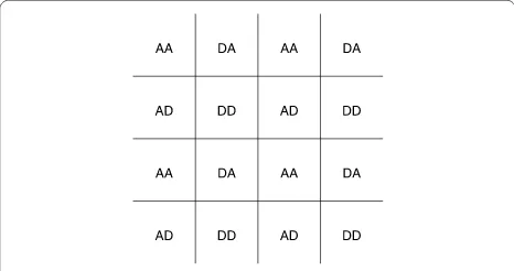
Based on the polyphase description in Figure , the lift-ing coefficients of the D implementation can be derived. The variablez corresponds to the vertical and z to the horizontal direction. The annotations DD, AD, DA, and
AAare related to the positions in Figure . The lettersA
andDdenote the D approximation signal (low-pass band) and the detail signal (high-pass band), respectively. In D,
Figure 2 Position of resulting sub-band coefficients on a grid.
they appear in pairs.DA, for example, denotes the posi-tions of D sub-band coefficients derived from horizontal low-pass filtering and vertical high-pass filtering,i.e. us-ing the two-dimensional filter (h[n]). The lifting filters areL(z) = ( +z),L(z) = ( +z), K(z) = ( +z–
), and K(z) = ( +z–
).
The actual number of rounding steps can be determined based on Figure . Rounding is required at each lifting step before the summation,i.e.eight times in total. The round-ing steps are interdependent, however. The horizontal dual steps, for instance, process values fromDDandDA posi-tions, which have already been affected by the rounding in previous primal steps. This possible accumulation of rounding errors continues in the second dimension of the image signal.
LetXandYbe the polyphase input and output vectors
X= ⎛ ⎜ ⎜ ⎝ DD AD DA AA ⎞ ⎟ ⎟
⎠, Y=
⎛ ⎜ ⎜ ⎝ DD AD DA AA ⎞ ⎟ ⎟ ⎠. ()
Then, the first two lifting steps can be denoted as
L=
⎛ ⎜ ⎜ ⎝
a
a
⎞ ⎟ ⎟ ⎠,
L=
⎛ ⎜ ⎜ ⎝
b
b
⎞ ⎟ ⎟ ⎠
()
witha=α·L(z) andb=β·K(z). After exchanging the
orientation using the permutation matrix
P= ⎛ ⎜ ⎜ ⎝ ⎞ ⎟ ⎟ ⎠, ()
another two lifting steps follow
L=
⎛ ⎜ ⎜ ⎝
a
a
⎞ ⎟ ⎟ ⎠,
L=
⎛ ⎜ ⎜ ⎝
b
b
⎞ ⎟ ⎟ ⎠
Y=
⎛ ⎜ ⎜ ⎝
a a a·a
b a·b+ a·b a·(a·b+ ) b a·b a·b+ a·(a·b+ ) bb b·(a·b+ ) b·(a·b+ ) (a·b+ )·(a·b+ )
⎞ ⎟ ⎟
⎠·X ()
Figure 3 Processing of 5/3-lifting decomposition.See text for details.
witha=α·L(z) andb=β·K(z). The entire processing is
Y= (P·L·L)·(P·L·L)·X, ()
leading to equation () in Figure .
In Figure , the single lifting steps are annotated with ei-therαorβ, expressing which of the two equations () or () is used (in one dimension). The D-lifting computation is derived from this signal flow as follows. IfX(z,z) cor-responds toxn,m, then we get the following equivalences:
AD•––◦xn,m–, DD•––◦xn,m,
DA•––◦xn–,m, AA•––◦xn–,m–.
With respect to Figure , the sub-band signals
DD(z,z)•––◦ddn,m, AD(z,z)•––◦adn,m–,
DA(z,z)•––◦dan–,m, AA(z,z)•––◦aan–,m–
are accordingly computed as follows. The two-dimensional detail signal is computed with
ddn,m=xn,m+α·(xn,m–+xn,m+)
+α·(xn–,m+xn+,m)
+α·xn–,m–+xn+,m–
+xn–,m++xn+,m+. () According to the processing structure of the lifting scheme, the signal values xn,m are now overwritten by
ddn,mand are not available anymore. Therefore, the next lifting step is
dan–,m=xn–,m+α·(xn–,m–+xn–,m+)
+β·(ddn–,m+ddn,m). ()
Since we know that the filter (h[n]) is the transpose of (h[n]), the computation of the AD path must analogously
be equal to
adn,m–=xn,m–+α·(xn–,m–+xn+,m–)
+β·(ddn,m–+ddn,m). ()
Based on these three relations we get
aan–,m–=xn–,m–
+β·(adn–,m–+adn,m–)
+β·(dan–,m–+dan–,m)
–β·(ddn–,m–+ddn–,m
+ddn,m–+ddn,m). ()
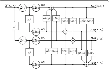
Consequently, the two-dimensional filtersh· · ·hcan be implemented directly using a D lifting structure. Fig-ure illustrates the processing steps.
Based on equations ()-(), it becomes obvious that only one single rounding step is required for each sub-band value in the D implementation. And, in fact, the scheme in Figure can be modified accordingly, reducing the total number of lifting steps from eight to four (Figure ). This corresponds to a factorization of equation () in merely three matrices, since signalsADandDAcan be computed concurrently
Y=Lβ·Lαβ·Lα·X ()
with
Lα=
⎛ ⎜ ⎜ ⎝
a a aa
⎞ ⎟ ⎟ ⎠,
Lαβ=
⎛ ⎜ ⎜ ⎝
b a b a
⎞ ⎟ ⎟ ⎠
Figure 4 General two-dimensional signal flow for 5/3 lifting: (a)-(d) first, second, third, and fourth lifting step.
and
Lβ=
⎛ ⎜ ⎜ ⎝
–bb b b
⎞ ⎟ ⎟
⎠. ()
Figure 5 Two-dimensional 5/3-lifting decomposition in z-domain with reduced number of lifting steps.
Section investigates the influence of the reduced num-ber of rounding steps on the performance of an IWT-based compression system.
3 JPEG2000 9/7 filter bank 3.1 One-dimensional decomposition
The standard / filter bank can be implemented based on the lifting scheme in the same manner as the / filter bank shown in the previous section. The only difference is that, in total, four lifting steps are needed in each direction ([], Figure ).
In literature, the factorization of a scaling factor is also discussed. We would like to remark that in the case of loss-less compression, this scaling is not necessary and would merely introduce more rounding operations degrading the performance of the wavelet transform. In lossy compres-sion, the scaling can be shifted into the quantization step, thus, there is no reason to treat the scaling within the transformation stage.
Further, it must be pointed out that for the practical im-plementation and in order to avoid an exception handling at the signal boundaries, it is sufficient to extend the origi-nal or intermediate sigorigi-nals by a single value at both bound-aries.
In application to image compression, the typical filter de-sign aims to achieve maximal flat magnitude responses at frequencyf = (high-pass filter) and at half of the sam-pling frequency (low-pass filter),i.e.a maximum number of vanishing moments is desired []. The / filters allow for vanishing moments each, thus the equations () hold true forp∈ {; ; ; }. These constraints lead to the follow-ing liftfollow-ing coefficients, eitherviafactorisation of the two-channel filter bank [] orviadirect filter design based on the lifting structure []
α≈–., γ ≈.,
Figure 6 Separable two-dimensional 9/7-lifting decomposition inz-domain.The symbol ‘x·’ is a short-cut forx·P(z) (see text for details).
3.2 Two-dimensional decomposition
The two-dimensional signal flow can be described in sim-ilar manner as the D / filter bank. Figure depicts the separable transformation without rounding steps. The annotation of primal and dual lifting steps withα,γ, β, andδ, relates to the subsequent lifting steps shown in [], Figure . For the sake of visualisation, the annotation withL(z),L(z),K(z), andK(z) is omitted. Its influence
should be clear by now. The coefficientsαandγ are asso-ciated withL(zk),βandδwithK(zk). The processing can
be denoted as
Y= (P·L·L·L·L)·(P·L·L·L·L)·X. ()
The four additional liftingL· · ·L steps are identical to
L· · ·Lin their structure, only the lifting coefficients are exchanged fromαtoγ andβtoδ.
The inner eight lifting steps encircled by the dotted line have the same structure as the / decomposition in Fig-ure
Y= (PLLP)·(PLLPLL)·(LL)·X. ()
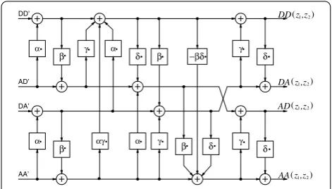
In [], it is suggested to substitute them, using the lifting structure of Figure , facilitating the reduction of round-ing steps. Figure shows the result. As can be seen, the first two lifting steps in the horizontal direction, as well as the last two steps in the vertical direction, remained un-touched. The number of rounding operations has been re-duced from four (Figure ) to only three per sub-band sam-ple.
It is, however, possible to reduce the number of rounding steps further by reordering the matrices
Y= (PLLPLL)·(PLLPLL)·X. ()
Figure 7 Two-dimensional 9/7-lifting decomposition in z-domain with reduced number of lifting steps.
The third and fourth lifting step of the horizontal de-composition of Figure can be moved to the end of the processing pipeline (Figure ). Now, both parts encir-cled by the dotted lines can be substituted using the lifting structure of Figure . The corresponding processing is
Y= (LδLγ δLγ)·(LβLαβLα)·X ()
with
Lγ =
⎛ ⎜ ⎜ ⎝
g g gg
⎞ ⎟ ⎟ ⎠,
Lγ δ=
⎛ ⎜ ⎜ ⎝
d g d g
⎞ ⎟ ⎟ ⎠
()
Figure 9 Two-dimensional 9/7-lifting decomposition in z-domain with only eight rounding steps.
and
Lδ=
⎛ ⎜ ⎜ ⎝
–dd d d
⎞ ⎟ ⎟
⎠, ()
with g=γ ·L(z), g=γ ·L(z),d=δ·K(z) andd= δ·K(z).
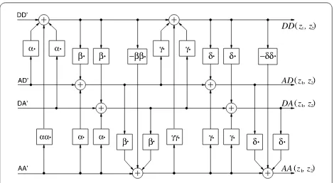
The new decomposition in Figure requires even fewer lifting steps and is still fully compatible with the conven-tional / filter bank (Figure ), when the rounding steps are left out. Now, only two steps per sub-band sample are required. The number of consecutive processing steps is even reduced from eight (Figure ) to six, since theADand
DAchannels can be computed at the same time. Iwahashi and Kiya developed this structure independently with the focus on the reduced latency of this D decomposition [].
4 Deslauriers-Dubuc 9/7 filter bank
In addition to the filter banks defined in the JPEG standard part I, the Deslauriers-Dubuc / filter bank (DD) is of interest in this context [, , ]. Its high-pass filter has four vanishing moments and the low-high-pass filter two. As the name suggests, the filters have and taps, respectively
h[n]
= – – ,
h[n]= –
–
. ()
The filter bank, however, can be implemented with only two lifting steps, similar to the / filter bank. In integer
arithmetic, the lifting steps are
dn=xn+
+xn–– ·(xn+xn+)
+xn++ , ()
an=xn+[xn+xn++ ]. () This makes the structure in Figure applicable for the DD filter bank as well. The only difference concerns fol-lowing lifting polynomials: L(z) = (z–
– – ·z+z)
andL(z) = (z– – – ·z+z) both in combination with
α= /. The other lifting steps remain K(z) = ( +z– ) andK(z) = ( +z–
) withβ= /.
The D lifting steps of the DD filter bank are imple-mented as
ddn,m=xn,m
+(xn,m–+xn,m+
+xn–,m+xn+,m) + (xn–,m–+xn–,m+
+xn+,m–+xn+,m+)·
–(xn–,m+xn+,m
+xn,m–+xn,m+) +xn–,m–+xn–,m+
+xn–,m–+xn–,m+
+xn+,m–+xn+,m+
+xn+,m–+xn+,m+· +xn–,m–+xn–,m+
+xn+,m–+xn+,m+
+ , ()
adn,m–=xn,m–
+(ddn,m–+ddn,m) +xn–,m–
– ·(xn–,m–+xn+,m–)
+xn+,m–+ , ()
dan–,m=xn–,m
+(ddn–,m+ddn,m) +xn–,m–
– ·(xn–,m–+xn–,m+)
aan–,m–=xn–,m–
+(adn–,m–+adn,m–
+dan–,m–+dan–,m)
– (ddn–,m–+ddn–,m
+ddn,m–+ddn,m) + . () 5 ‘Rounding-friendly’ lifting coefficients
The superiority of the separable / filters over the separa-ble standard / IWT filter bank, documented in literature [, , ], has its reason in the minimal accumulated influ-ence of rounding at each lifting step, leading to a minimal change in the filter characteristics. Not only is the number of steps lower (only two instead of four in each direction), but the rounding error in its first lifting step is also smaller, since the factor ofα= –/ only results in errors when the sum ofxmandxm+is odd (see eq. ()). The degradation
of the magnitude response of the standard / filter is dis-tinctly higher.
With this degradation in mind, we investigated whether some of the filter-design constraints leading to a maximum number of vanishing moments can be released, to obtain lifting coefficients which introduce fewer rounding errors, while keeping the essential characteristic of the magnitude responses.
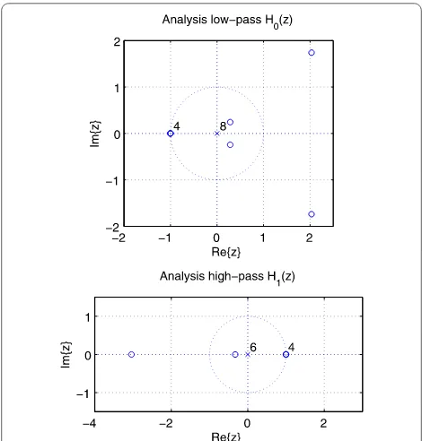
Introducing a maximal number of vanishing moments as realized with equation () corresponds to a maximum number of zeros atz= – for the analysis low-pass filter
H(z) and atz= for the analysis high-pass filterH(z)
(Figure ). The corresponding lifting coefficients have al-ready been shown in equation ().
In general, the relaxation of these filter constraints leads to poorer decorrelation of the input image. If, however, the adverse effects of rounding decrease due to the modifica-tion of the lifting coefficients, then there might be an opti-mal compromise. Reducing the number of vanishing mo-ments from four to two increases the degree of freedom in selecting lifting coefficients with suitable properties.
Inspecting the flow chart in Figure , it becomes obvi-ous that the first lifting step has the greatest influence on the non-linear filter characteristic. All rounding errors in-troduced at this point are likely to propagate through the entire lifting cascade. Consequently, it is desirable to find a set of lifting coefficients leading to similar magnitude re-sponses as the original coefficients in eq. (), but withα equal to – avoiding any rounding error in the first lifting step. A promising set of lifting coefficients was found in [] with
α= –, β= –
√
,
γ=
√
–
, δ=
.
()
Figure 10 Location of zeros and poles of the standard 9/7 wavelet filter.
The approximation to
α= –, β= –
, γ=
, δ=
()
allows a division-free implementation in integer arith-metic as follows
ddn,m
=xn,m
– (xn–,m+xn+,m+xn,m–+xn,m+)
+ (xn–,m–+xn–,m+
+xn+,m–+xn+,m+) ()
adn,m–
=xn,m–
– (xn–,m–+xn+,m–)
–·ddn,m– +ddn,m+ ()
dan–,m
=xn–,m
– (xn–,m–+xn–,m+)
aan–,m–
=xn–,m–
–·adn–,m–+adn,m–
+dan–,m–+dan–,m
+ ·ddn–,m– +ddn–,m
+ddn,m– +ddn,m+ ,, ()
ddn,m=ddn,m
+,·dan–,m+dan+,m
+adn,m–+adn,m+
+ ,·aan–,m–+aan–,m+
+aan+,m–+aan+,m+
+ , ()
adn,m–
=adn,m–
+·aan–,m–+aan+,m–
+(ddn,m–+ddn,m)+ ()
dan–,m
=dan–,m
+·aan–,m–+aan–,m+
+(ddn–,m+ddn,m)+ ()
aan–,m–=aan–,m–
+(adn–,m–+adn,m–
+dan–,m–+dan–,m)
– (ddn–,m–+ddn–,m
+ddn,m–+ddn,m) + . ()
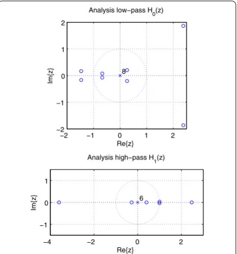
The corresponding filters have no real vanishing mo-ments. Figure shows that in comparison to Figure , zeros have moved from their original location on the unit circle to other places.
6 Investigations
6.1 Effects of rounding in 1D
The effects of rounding on the impulse responses of the high and low-pass filters have been investigated in the fol-lowing manner.
The convolution
y[n] =h[n] *v·x[n]
Figure 11 Location of zeros and poles of the 9/7 wavelet filter with relaxed constraints enabling division-free integer arithmetic.
was computed with (x[n]) equal to the Kronecker deltaδ[k] as input signal. The convolution result is therefore equal to
v·h[n–k] =h[n] *v·x[n].
If, however, the rounding to integer values is additionally performed, then the result is notv·h[n–k], butv·h[n–k]. When using an impulse magnitude ofv= and settingk= , for example, the designed impulse responses of the / decomposition change from eq. () to
h[n]=– –/,
h[n]=– –/.
In case of the standard / filters, the impulse responses change from
h[n]= (. –. –.
. –. · · ·),
h[n]= (. –. –.
. . . · · ·)
to
Figure 12 Change of magnitude response caused by rounding: (a) 5/3 filter bank; (b) 9/7 Deslauriers-Dubuc filter bank; (c) 9/7 filter bank; (d) 9/7 filter bank with lifting coefficients from eq. (39) (solid: transfer function without rounding; dash, dash-dot, and dot indicate signal valuesvof 31, 15, and 9 used for determination of the impulse responses with rounding).
h[n]= /. Figure shows the corresponding magnitude responses depending on the valuevof the single impulse functioning as input signal.
The smaller the input valuev, the higher the effect of rounding.
6.2 Effects of rounding in 2D
In order to illustrate the rounding effects in two dimen-sions, the same procedure as in the previous section was performed, but with the distinction that D filters were used.
.. Effects in the / filter bank
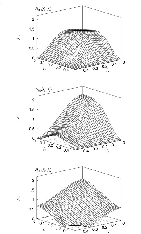
Figure (a) depicts the original magnitude response of the / filter (h[n]) from eq. (). The frequency axes are nor-malised by the sampling frequency. If rounding is applied, the magnitude response changes (Figure (b)). In this and subsequent investigations, the impulse magnitude used as input signal was always set equal tov= .
In general, the resulting impulse responses depend on the processing structure. In the particular case of v= however, theh,h, andhfilters are the same for both
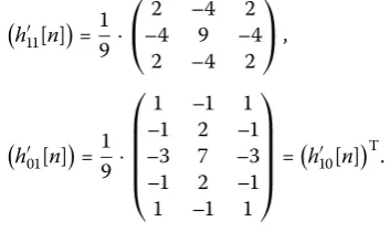
(Figure or from Figure ). The impulse responses from eqs. ()-() change in both cases to
h[n]= ·
⎛
⎝– – –
–
⎞ ⎠,
h[n]= ·
⎛ ⎜ ⎜ ⎜ ⎜ ⎝
–
– –
– –
– –
–
⎞ ⎟ ⎟ ⎟ ⎟ ⎠=
h[n]T.
Figures (c) and (d) compare the original with the de-formed magnitude responses for the filterh.
Figure 13 5/3 filter bank: distorted magnitude response caused by rounding to integer values; (a) original magnitude responseH11(fx,fy);
(b) separable/2D implementationH11(fx,fy) (Figures 1 and 5); (c) original magnitude responseH01(fx,fy); (b) separable/2D
implementationH01(fx,fy).
The two-dimensional impulse responses from () dete-riorate to
h[n]sep= · ⎛ ⎜ ⎜ ⎜ ⎜ ⎝ – – ⎞ ⎟ ⎟ ⎟ ⎟ ⎠.
in case of the separable implementation and to
h[n]D= · ⎛ ⎜ ⎜ ⎜ ⎜ ⎝ ⎞ ⎟ ⎟ ⎟ ⎟ ⎠.
in case of the D implementation.
.. Effects in the / filter bank
For the case of the standard / filter bank, we have to compare three different implementations, which are called ‘v’, ‘v’, and ‘v’ in the following, according to the flow charts in Figures , , and , respectively.
The h impulse response changes from the matrix
shown in Figure to following
h[n]v= · ⎛ ⎜ ⎜ ⎜ ⎜ ⎜ ⎝ – – – – – .. . ... ... ... ... ... ... ⎞ ⎟ ⎟ ⎟ ⎟ ⎟ ⎠ ,
h[n]v= · ⎛ ⎜ ⎜ ⎜ ⎜ ⎜ ⎝ – – – .. . ... ... ... ... ... ... ⎞ ⎟ ⎟ ⎟ ⎟ ⎟ ⎠ ,
h[n]v= · ⎛ ⎜ ⎜ ⎜ ⎜ ⎜ ⎝ – – – .. . ... ... ... ... ... ... ⎞ ⎟ ⎟ ⎟ ⎟ ⎟ ⎠ .
The magnitude of the input impulse was again equal to
Figure 14 5/3 filter bank: distorted magnitude response of H00(fx,fy) caused by rounding to integer values; (a) original
magnitude response; (b) separable implementation (Figure 1); (c) 2D implementation (Figure 5).
from the matrices above. The graph of the correspond-ing magnitude responses underlines this observation (Fig-ure ).
Similar alterations of the filter coefficients can be ob-served for theh,h, andh filters. Another effect of non-linearity is that thehfilters are no longer the trans-poses of thehfilters.
Comparing the similarities of the two-dimensional im-pulse responses between the different implementations, the deviation is higher for thehandhfilters than for thehfilter. This continues for thehfilter, which shows the highest variation from one implementation to another. Using the new lifting coefficients, the degradation of the filters is generally reduced (Figure in comparison with Figure ).
Note that the degradation is dependent on the magni-tude of the impulse functioning as input signal. The shown magnitude responses merely give an impression of the ef-fects, but do not allow a general conclusion or even a the-oretical analysis.
6.3 Efficiency of decorrelation
The efficiency of the different filter banks was first analysed based on the zero-order entropies of single sub-bands.
Table -Table contain the zero-order entropies of the sub-bands DD, AD, DA and AA after one D de-composition step is applied to different grey-scale im-ages. Barbara-Zelda are taken from [], cats_g-educ from []. kodim-kodim are the green components of true colour images found at []. The meaning of the column titles is
– v: / filter bank, implementation of Figure , – v: / filter bank, implementation of Figure , – D: / Deslauriers-Dubuc, implementation of
Figure ,
– D: / Deslauriers-Dubuc, implementation of Figure ,
– v: / filter bank, implementation of Figure , – v: / filter bank, implementation of Figure , – v: / filter bank, implementation of Figure , – va - va: same as before, but with lifting
coefficients from equation ().
The numbers in bold denote the best (smallest) value in each entire row. In each category (/, Deslauriers-Dubuc, /, / with modified coefficients), the best value is un-derlined.
While the explanations in Section were given with im-plicit floating-point arithmetic plus rounding operation (eqs. (), (), and ()–()), the practical implementation of the / filter banks (v, v) is based on plain integer arithmetic as follows
dn=xn+–(xn+xn+), (∗)
an=xn+(xn+xn++ ), (∗)
ddn,m=xn,m
+xn–,m–+xn+,m–
+xn–,m++xn+,m+
–(xn,m–+xn,m++xn–,m
+xn+,m)+ , (∗)
dan–,m=xn–,m
+ddn–,m+ddn,m
–(xn–,m–+xn–,m+)
h[n]≈ ·
⎛ ⎜ ⎜ ⎜ ⎜ ⎜ ⎝
. –. –. . –. –. .
–. . . –. . . –.
–. . . –. . . –.
. –. –. . –. –. .
..
. ... ... ... ... ... ...
⎞ ⎟ ⎟ ⎟ ⎟ ⎟ ⎠
h[n]≈ ·
⎛ ⎜ ⎜ ⎜ ⎜ ⎜ ⎜ ⎜ ⎝
. –. –. . –. –. .
–. . . –. . . –.
–. . . –. . . –.
. –. –. . –. –. .
. –. –. . –. –. .
..
. ... ... ... ... ... ...
⎞ ⎟ ⎟ ⎟ ⎟ ⎟ ⎟ ⎟ ⎠
h[n]=h[n]T
h[n]≈ ·
⎛ ⎜ ⎜ ⎜ ⎜ ⎜ ⎜ ⎜ ⎝
. –. –. . . . –. –. .
–. . . –. –. –. . . –.
–. . . –. –. –. . . –.
. –. –. . . . –. –. .
. –. –. . . . –. –. .
..
. ... ... ... ... ... ... ... ...
⎞ ⎟ ⎟ ⎟ ⎟ ⎟ ⎟ ⎟ ⎠
Figure 15 Two-dimensional impulse responses of the original 9/7 filter bank.The matrices are symmetric in the horizontal and vertical directions. The factor 1/9 is extracted for better comparison with numbers in the text.
Figure 16 9/7 filter bank: distorted magnitude response ofH11(fx,fy) caused by rounding; (a) original magnitude response; (b) 97v1
Figure 17 9/7 filter bank with modified lifting coefficients (eq. (39)): distorted magnitude response ofH11(fx,fy) caused by
rounding; (a) original magnitude response; (b) 97v1a implementation; (c) 97v2a implementation; (d) 97v3a implementation.
adn,m–=xn,m–
+ddn,m–+ddn,m
–(xn–,m–+xn+,m–)
+ , (∗)
Figure 18 9/7 filter bank with modified lifting coefficients (eq. (39)): distorted magnitude response ofH00(fx,fy) caused by
rounding; (a) original magnitude response; (b) 97v1a implementation; (c) 97v2a implementation; (d) 97v3a implementation.
aan–,m–=xn–,m–
+(adn–,m–+adn,m–
+dan–,m–+dan–,m) – (ddn–,m–+ddn–,m
Table 1 DD-band entropies in bit per pixel after first decomposition
Image 53v1 53v2 97D1 97D2 97v1 97v2 97v3 97v1a 97v2a 97v3a
barbara.y 4.503 4.494 4.427 4.415 4.218 4.202 4.206 4.235 4.230 4.223 barbara2.y 4.765 4.746 4.834 4.819 4.595 4.578 4.577 4.553 4.536 4.532
black.y 3.716 3.708 3.828 3.814 3.550 3.529 3.537 3.470 3.466 3.450
boats.y 3.795 3.791 3.873 3.865 3.611 3.598 3.605 3.548 3.548 3.536
goldhill.y 4.361 4.348 4.469 4.461 4.203 4.190 4.192 4.137 4.130 4.125
zelda.y 3.961 3.961 4.094 4.091 3.785 3.775 3.778 3.697 3.702 3.696
cats_g 3.098 3.083 3.100 3.086 2.967 2.952 2.970 2.958 2.942 2.937
bike 4.098 4.087 4.163 4.147 4.000 3.967 3.979 3.933 3.918 3.905
educ 3.717 3.707 3.610 3.588 3.537 3.525 3.531 3.529 3.523 3.507
kodim07 3.478 3.463 3.582 3.551 3.451 3.377 3.425 3.350 3.323 3.292
kodim08 4.933 4.930 5.009 5.008 4.794 4.792 4.792 4.743 4.742 4.740
kodim09 3.842 3.837 3.938 3.931 3.728 3.711 3.722 3.655 3.654 3.642
average 4.022 4.013 4.077 4.065 3.870 3.850 3.860 3.817 3.810 3.800
Table 2 AD-band entropies in bit per pixel after first decomposition
Image 53v1 53v2 97D1 97D2 97v1 97v2 97v3 97v1a 97v2a 97v3a
barbara.y 4.202 4.198 3.853 3.846 3.960 3.961 3.971 4.087 4.093 4.081 barbara2.y 4.231 4.239 4.108 4.113 4.169 4.172 4.178 4.190 4.197 4.188 black.y 3.438 3.423 3.280 3.273 3.472 3.471 3.487 3.468 3.468 3.451 boats.y 3.733 3.718 3.547 3.515 3.734 3.716 3.736 3.753 3.749 3.732 goldhill.y 4.492 4.528 4.443 4.470 4.553 4.581 4.582 4.554 4.587 4.580 zelda.y 3.147 3.120 3.024 3.001 3.132 3.117 3.132 3.114 3.103 3.084 cats_g 3.348 3.341 3.255 3.245 3.332 3.329 3.338 3.360 3.371 3.364 bike 4.613 4.598 4.611 4.596 4.737 4.730 4.740 4.710 4.705 4.698 educ 4.989 4.983 4.733 4.721 4.939 4.935 4.939 5.031 5.028 5.026 kodim07 4.031 4.045 3.801 3.823 3.982 4.018 4.031 4.044 4.071 4.057 kodim08 5.672 5.644 5.696 5.679 5.806 5.786 5.789 5.780 5.754 5.753 kodim09 4.169 4.150 4.146 4.124 4.255 4.237 4.250 4.234 4.220 4.212 average 4.172 4.166 4.041 4.034 4.173 4.171 4.181 4.194 4.196 4.186
The results for the DD band (high-pass filtering in both directions) show a clear trend with decreasing entropy from left to right (Table ), when excluding D and D. There is only one exception: the implementation v leads to lower entropy on average than v when the standard lifting coefficients (eq. ()) are used. The Deslauriers-Dubuc filter bank (D) performs worst de-spite the four vanishing moments of its high-pass filter. One reason lies in the gain ofH(z)|z=–= , which is sig-nificantly higher than the gain of the JPEG / high pass. In comparison to the / filter banks (also having
H(–) = ), the filter characteristic seems to be more in-fluenced by the rounding operations deteriorating the ad-vantage of two additional vanishing moments.
The D implementations of the / filter bank (v) and of the Deslauriers-Dubuc filter bank (D) are superior to the separable implementations. All other / implementa-tions yield better results, despite the higher number of lift-ing steps. It also can be seen that the modified liftlift-ing coef-ficients truly improve the decorrelation on average. How-ever, the numbers in this table also reveal that the num-ber of rounding steps is not a unique measure to estimate
the influence of rounding steps. The DD values depend on three steps in v and only on two steps in v; never-theless, the result is better for v.
Table draws another picture. The implementations v, D, v, and va are again the winner within their categories. The filter banks based on only two lift-ing steps, however, lead to the smaller entropies in the AD band on average. Surprisingly, the results for the DA band in Table are not very similar to the values for the AD band. Very interesting, although not in the primary scope of this paper, is the fact that all images taken from [] have a higher entropy in the DA band compared to the AD band. The vertical edges are obviously sharper than the horizon-tal ones. Using rotated versions of the images reverses the results. It might be that the point spread function of the camera system used for taking these pictures was not sym-metric. This can also cause the / filter bank to perform better for the DA band than for the AD band. Short filters are more suitable at pronounced edges.
al-Table 3 DA-band entropies in bit per pixel after first decomposition
Image 53v1 53v2 97D1 97D2 97v1 97v2 97v3 97v1a 97v2a 97v3a
barbara.y 5.431 5.449 5.383 5.389 5.460 5.473 5.480 5.475 5.485 5.490 barbara2.y 5.537 5.531 5.539 5.541 5.617 5.623 5.626 5.607 5.600 5.602 black.y 4.005 4.070 4.055 4.077 4.114 4.158 4.173 4.063 4.115 4.126 boats.y 4.471 4.490 4.492 4.492 4.574 4.593 4.603 4.552 4.559 4.564 goldhill.y 4.582 4.585 4.584 4.584 4.647 4.657 4.660 4.639 4.637 4.638 zelda.y 4.062 4.087 4.072 4.076 4.124 4.139 4.151 4.109 4.123 4.125 cats_g 3.445 3.423 3.350 3.339 3.428 3.460 3.432 3.444 3.456 3.454 bike 4.507 4.503 4.501 4.496 4.577 4.609 4.618 4.567 4.569 4.577 educ 4.734 4.708 4.450 4.445 4.609 4.633 4.648 4.724 4.725 4.730 kodim07 3.627 3.614 3.557 3.548 3.660 3.733 3.755 3.665 3.664 3.683 kodim08 5.814 5.812 5.837 5.831 5.960 5.955 5.957 5.936 5.926 5.928 kodim09 4.046 4.061 4.039 4.047 4.115 4.143 4.162 4.093 4.103 4.112 average 4.522 4.528 4.488 4.489 4.574 4.598 4.605 4.573 4.580 4.586
Table 4 AA-band entropies in bit per pixel after first decomposition
Image 53v1 53v2 97D1 97D2 97v1 97v2 97v3 97v1a 97v2a 97v3a
barbara.y 7.563 7.558 7.553 7.538 8.119 8.113 8.109 8.100 8.097 8.090 barbara2.y 7.504 7.495 7.490 7.483 8.047 8.055 8.045 8.031 8.025 8.027 black.y 6.759 6.744 6.773 6.744 7.372 7.342 7.360 7.330 7.327 7.316 boats.y 7.111 7.097 7.103 7.082 7.669 7.659 7.672 7.646 7.645 7.647 goldhill.y 7.556 7.548 7.551 7.537 8.127 8.134 8.127 8.103 8.099 8.099 zelda.y 7.332 7.334 7.330 7.319 7.912 7.916 7.915 7.884 7.897 7.888 cats_g 4.738 4.740 4.732 4.734 5.008 5.020 5.023 5.006 5.007 5.010 bike 7.429 7.430 7.396 7.396 7.918 7.925 7.929 7.919 7.920 7.920 educ 7.449 7.448 7.446 7.445 8.041 8.044 8.047 8.017 8.019 8.017 kodim07 7.139 7.147 7.114 7.121 7.672 7.677 7.680 7.662 7.669 7.667 kodim08 7.822 7.828 7.794 7.800 8.333 8.333 8.332 8.320 8.320 8.321 kodim09 7.237 7.246 7.223 7.232 7.793 7.801 7.802 7.776 7.782 7.784 average 7.137 7.135 7.125 7.119 7.668 7.668 7.670 7.650 7.651 7.649
most the same. The superior results for the / and DD filter banks are also caused by the lower amplification of the low-pass filter (see Figure ). While their low-pass fil-ter transfer functionH(z) is equal to atz= , the amplifi-cation for the JPEG / low pass is about . affect-ing also the D characteristics (compare Figures a and a).
In addition, we would like to point out that the modified lifting coefficients again have a positive influence on the decorrelation.
6.4 Compression results
The overall performance of the different filter banks was tested in combination with a compression system, which applies the basic coding algorithm of JPEG without using the header/marker structure. The number of decom-position steps was dependent on the image size, for exam-ple, five decompositions for images with × pixels
and seven decompositions for images with ×
pixels. The focus was exclusively on lossless image com-pression. A rate-distortion analysis exploiting the scalabil-ity of the compression scheme is not considered in this pa-per.
When comparing the lossless compression results in bits per pixel (Table ), the superiority of the D implementa-tion of the / Deslauriers-Dubuc filter bank becomes ap-parent. There is also only a single case (goldhill.y) where the separable / implementation is better than any D im-plementation. Only in cases of special image texture (bar-bara.y, cats_g, and educ) can a standard / implementa-tion compete with the / filter banks.
The v(a) implementation does not result in any ad-vantage over the separable v(a) implementation. The new non-separable implementation va in combination with the lifting coefficients according to eq. () performs best within all / filter banks based on the JPEG / filter-bank structure.
6.5 Complexity of implementations
compu-Table 5 Compression results in bits per pixel [bpp]
Image 53v1 53v2 97D1 97D2 97v1 97v2 97v3 97v1a 97v2a 97v3a
barbara.y 4.594 4.584 4.478 4.469 4.538 4.535 4.549 4.558 4.563 4.556 barbara2.y 4.778 4.776 4.737 4.744 4.777 4.793 4.802 4.769 4.772 4.772 black.y 3.765 3.750 3.774 3.750 3.854 3.844 3.864 3.796 3.796 3.786 boats.y 4.057 4.033 4.024 3.991 4.104 4.095 4.117 4.075 4.070 4.059 goldhill.y 4.593 4.595 4.594 4.596 4.633 4.650 4.656 4.618 4.620 4.616 zelda.y 3.870 3.850 3.853 3.834 3.912 3.901 3.920 3.876 3.872 3.864 cats_g 2.542 2.534 2.500 2.493 2.527 2.532 2.541 2.537 2.539 2.537 bike 4.364 4.342 4.343 4.324 4.412 4.409 4.431 4.387 4.383 4.373 educ 4.534 4.513 4.342 4.315 4.493 4.490 4.512 4.534 4.530 4.515 kodim07 3.777 3.741 3.715 3.687 3.846 3.850 3.888 3.814 3.809 3.794 kodim08 5.531 5.516 5.539 5.533 5.572 5.568 5.574 5.553 5.544 5.545 kodim09 4.027 4.013 4.027 4.012 4.092 4.090 4.116 4.054 4.053 4.046 average 4.203 4.187 4.161 4.146 4.230 4.230 4.248 4.214 4.213 4.205
Table 6 Complexity estimation for different filter-bank implementations
Filter bank Adds Shifts Mults
53v1 20 8 0
53v2 28 8 0
97D1 32 8 4
97D2 48 9 4
97v1a 40 12 8 97v2a 47 11 10 97v3a 55 10 8
tation of four sub-band values for the investigated filter-bank structures. The numbers have been determined as follows. The implementation of v is based on equations (∗) and (∗). There are five adds and two shifts. To com-pute four sub-band values, both equations have to be ap-plied two times horizontally and two times vertically, lead-ing to a total number of twenty adds and eight shifts. Equa-tions (∗)-(∗) compute four sub-band values according to the D structure v. There are + + + = adds and + + + = shift operations. Filter bank D is based on equations () and (), requiring eight adds, two shifts and one integer multiplication. Again, these num-bers must be multiplied by four. Equations ()-() reflect the complexity of filter bank D. There are +++ = adds, nine shift operations and four integer multiplica-tions.
The numbers for filter banks va, va and va have been derived from their implementations (see also eqs. ()-()).
It can be noticed that the increase of complexity is rather moderate when switching from a one-dimensional to a two-dimensional implementation. This is largely due to the properties of the lifting scheme and the utilisation of the symmetry of filters. With respect to the memory ac-cess, the D implementation is even somewhat advanta-geous, as the algorithm runs only once through the data
and not twice, separately in horizontal and vertical di-rections. Practical implementations, however, also have to consider the efforts of signal extension at the signal bound-aries, which are highest for the Dx filter banks.
7 Summary and conclusions
The paper has discussed and analysed different attempts to decrease the effects of rounding in implementations of the integer wavelet transform. The number of rounding steps could be reduced practically by special two-dimensional implementations of the / and / filter banks and vir-tually by using a first lifting coefficient ofα = – in the JPEG / filter bank. Dependent on the implemen-tation, the rounding of intermediate values to integers has different effects on the impulse responses and, conse-quently, on the decomposition of the signal.
The set of test images contained twelve natural images. It can be shown that the various processing schemes af-fect the single sub-bands differently in terms of entropy. As soon as the low-pass filter comes into play, the / fil-ter bank and the DD filfil-ter bank tend to decorrelate the image data better than the standard / filter bank and its derivatives. The gain of the low-pass filter atz= has a high impact on lossless compression performance.
The compression results of the / and DD filter bank have been improved on average by substituting the sepa-rable implementation with a special D processing, which would be compatible in the absence of rounding. The mere reduction of rounding steps by D implementations of the JPEG / filter bank does not lead to increased compression ratios. Only when the modified lifting coef-ficients enabling division-free integer arithmetic are com-bined with the new proposed D implementation does the average bitrate of the compressed images decrease from . bpp to . bpp. This is about the same bitrate as for the standard / filter bank while having distinctly higher complexity.
solely determined by the number of lifting steps, which means the rounding errors (strictly: their variances) do not simply sum up. The degradation of the filter characteristics under the presence of rounding also depends on the values of the lifting coefficients and on the structure of process-ing. The best compression result could be obtained with the new D implementation of the / Deslauriers-Dubuc filter bank (D). It requires only two sequential lifting steps as the / filter bank, while having more suitable fil-ter characfil-teristics. The improvement is .% compared to the standard / implementation (v) for the set of images used.
Competing interests
The authors declare that they have no competing interests.
Acknowledgements
The authors would like to thank the unknown reviewers who gave valuable comments on an earlier version of this manuscript.
Received: 26 May 2011 Accepted: 11 March 2012 Published: 4 April 2012
References
1. JE Fowler, B Pesquet-Popescu, An overview on wavelets in source coding, communications, and networks. EURASIP J. Image Video Coding2007, Article ID 60539 (2007)
2. W Sweldens, The lifting scheme: a new philosophy in biorthogonal wavelet construction, inProc. of SPIE, vol. 2569, San Diego, USA, July 1995, pp. 68–79
3. AR Calderbank, I Daubechies, W Sweldens, Y Boon-Lock, Lossless image compression using integer to integer wavelet transforms, inProc. of ICIP, vol. 1, 26-29 Oct. 1997, pp. 596–599
4. ISO/IEC JTC1/SC29/WG11 N1890, Information technology - JPEG 2000 Image Coding System. JPEG 2000 Part I, Final Draft Intern. Standard 15444, 25 Sep. 2000
5. F Sheng, A Bilgin, PJ Sementilli, MW Marcellin, Lossy and lossless image compression using reversible integer wavelet transforms, inProc. of ICIP, vol. 3, Los Alamitos, CA, USA (1998), pp. 876–880
6. VK Heer, H-E Reinfelder, A comparison of reversible methods for data compression, inProc. of SPIE - Medical Imaging IV, vol. 1233 (1990), pp. 354–365
7. A Said, WA Pearlman, An image multiresolution representation for lossless and lossy image compression. IEEE Trans. Image Process.5(9), 1303–1310 (1996)
8. A Zandi, JD Allen, EL Schwartz, M Boliek, CREW: compression with reversible embedded wavelets, inProc. of DCC, Snowbird, Utah, USA, 28-30 Mar 1995, pp. 212–221
9. MD Adams, F Kossentini, Reversible integer-to-integer wavelet transforms for image compression: performance evaluation and analysis. IEEE Trans. Image Process.9(6), 1010–1024 (2000)
10. J Reichel, G Menegaz, MJ Nadenau, M Kunt, Integer wavelet transform for embedded lossy to lossless image compression. IEEE Trans. Image Process. 10(3), 383–392 (2001)
11. M Grangetto, E Magli, M Martina, G Olmo, Optimization and
implementation of the integer wavelet transform for image coding. IEEE Trans. Image Process.11(6), 596–604 (2002)
12. D Sersic, Integer to integer mapping wavelet filter bank with adaptive number of zero moments, inProc. of ICASSP, vol. 1, Istanbul, Turkey, 9 June 2000, pp. 480–483
13. AT Deever, SS Hemami, Lossless image compression with
projection-based and adaptive reversible integer wavelet transforms. IEEE Trans. Image Process.12(5), 489–499 (2003)
14. H Li, G Liu, Z Zhang, Optimization of integer wavelet transforms based on difference correlation structures. IEEE Trans. Image Process.14(11), 1831–1847 (2005)
15. GCK Abhayaratne, G Piella, B Pesquet-Popescu, H Heijmans, Adaptive integer-to-integer wavelet transforms using update lifting, inProc. of SPIE, vol. 5207 (2003), pp. 813–824
16. GCK Abhayaratne, Spatially adaptive integer lifting with no side information for lossless video coding, inProc. Picture Coding Symposium (PCS), St. Malo, France, April 2003, pp. 495–500
17. ÖN Gerek, AE Cetin, An edge-sensing predictor in wavelet lifting structures for lossless image coding. EURASIP J. Image Video Coding2007, Article ID 19313 (2007)
18. J Solé, P Salembier, Generalized lifting prediction optimization applied to lossless image compression. IEEE Signal Process. Lett.14(10), 695–698 (2007)
19. V Kitanovski, M Kseneman, D Gleich, D Taskovski, Adaptive lifting integer wavelet transform for lossless image compression, inProc. of IWSSIP, Bratislava, Slovakia, 25-28 June 2008
20. DBH Tay, A class of lifting based integer wavelet transform, inIEEE Int. Conf. on Image Processing, vol. 1, Thessaloniki, Greece, 07-10 Oct. 2001, pp. 602–605
21. Z Guangjun, C Lizhi, C Huowang, A simple 9/7-tap wavelet filter based on lifting scheme. IEEE Int. Conf. Image Process.2, 249–252 (2001) 22. S Barua, KA Kotteri, AE Bell, JE Carletta, Optimal quantized lifting
coefficients for the 9/7 wavelet, inICASSP’04, vol. 5, 17-21 May 2004, pp. 193–196
23. T Strutz, Wavelet filter design based on the lifting scheme and its application in lossless image compression. WSEAS Trans. Signal Process. 5(2), 53–62 (2009)
24. M Iwahashi, H Kiya, Non separable 2D factorization of separable 2D DWT for lossless image coding, inProc. of ICIP, Cairo, Egypt, 7-11 Nov 2009, pp. 17–20
25. M Iwahashi, H Kiya, A new lifting structure of non separable 2D DWT with compatibility to JPEG 2000, inProc. of ICASSP, Dallas, Texas, USA, 14-19 March 2010, pp. 1306–1309
26. T Strutz, Design of three-channel filter banks for lossless image compression, inProc. of ICIP, Cairo, Egypt, 7-11 Nov 2009, pp. 2841–2844 27. D Le Gall, A Tabatabai, Sub-band coding of digital images using symmetric
short kernel filters and arithmetic coding techniques, inProc. of ICASSP, New York, NY, USA, 11-14 Apr 1988, pp. 761–764
28. G Deslauriers, S Dubuc, Symmetric iterative interpolation process. Constr. Approx.5, 49–68 (1989)
29. G Strang, T Nguyen,Wavelets and Filter Banks(Wellesley-Cambridge Press, Wellesley, 1996)
30. L Cheng, DL Liang, ZH Zhang, Popular biorthogonal wavelet filtersviaa lifting scheme and its application in image compression. IEE Proc., Vis. Image Signal Process.150(4), 227–232 (2003)
31. M Antonini, M Barlaud, P Mathieu, I Daubechies, Image coding using wavelet transform. IEEE Trans. Image Process.1(2), 205–220 (1992) 32. I Daubechies, W Sweldens, Factoring wavelet transform into lifting steps. J.
Fourier Anal. Appl.4(3), 247–269 (1998)
33. www1.hft-leipzig.de/strutz/Papers/Testimages/Bath-AC-UK/bath.html, Dezember 2010 (copied from the former web page
www.bath.ac.uk/elec-eng/research/sipg/resource/images.htm) 34. ITU-T Recommendation T.24: Standardized digitized image set, Version 3,
1998
35. http://r0k.us/graphics/kodak, Dec. 2009
doi:10.1186/1687-6180-2012-75
Cite this article as:Strutz and Rennert:Two-dimensional integer wavelet
transform with reduced influence of rounding operations.EURASIP Journal