Efficient Analysis of Time-Varying Multicomponent
Signals with Modified LPTFT
Yongmei Wei
School of Electrical and Electronic Engineering, Nanyang Technological University, Singapore 639798 Email:[email protected]
Guoan Bi
School of Electrical and Electronic Engineering, Nanyang Technological University, Singapore 639798 Email:[email protected]
Received 19 May 2004; Revised 13 October 2004; Recommended for Publication by Yuan-Pei Lin
This paper presents efficient algorithms for the analysis of nonstationary multicomponent signals based on modified local poly-nomial time-frequency transform. The signals to be analyzed are divided into a number of segments and the desired parameters for computing the modified local polynomial time-frequency transform in each segment are estimated from polynomial Fourier transform in the frequency domain. Compared to other reported algorithms, the length of overlap between consecutive segments is reduced to minimize the overall computational complexity. The concept of adaptive window lengths is also employed to achieve a better time-frequency resolution for each component. Numerical simulations with synthesized multicomponent signals show that the proposed ones achieve better performance on instantaneous frequency estimation with greatly reduced computational complexity.
Keywords and phrases:time-frequency analysis, time varying, multicomponent, modified LPTFT, impulse noise.
1. INTRODUCTION
Due to their superior performance in dealing with non-stationary signals, time-frequency transforms (TFTs) have found various applications in many areas including commu-nications, multimedia, mechanics, and biology [1]. The most popular and simplest TFT is short-time Fourier transform (STFT) that has been widely used for many practical applica-tions [1,2]. Nevertheless, the STFT suffers from low resolu-tion when the analyzed signal is highly nonstaresolu-tionary. Local polynomial time-frequency transform (LPTFT), referred to as the generalization of STFT, was reported to provide high resolution for nonstationary signals [3,4] with a local poly-nomial function approximating to the frequency character-istics. Unfortunately, the estimation of a number of extra pa-rameters required by LPTFT computation results in a heavy computational load. This is mainly due to the long overlap between consecutive signal segments for which the estima-tion process is implemented [4]. In order to reduce the com-putational complexity, attempts can be made to reduce the length of overlap between the consecutive segments. How-ever, problems of reduced resolution in the time-frequency domain have to be solved by using more effective methods of window length selection.
This paper presents analysis algorithms for time-varying multicomponent signals containing white Gaussian and/or impulse noises. Different from previously reported algo-rithms, the proposed modified local polynomial time-frequency transform (MLPTFT) reduces the overlap length between consecutive segments to minimize the number of segments to be processed. Effective methods of estimating the MLPTFT parameters from each signal segment are pre-sented. Deterioration of resolution due to the reduction of overlap length is avoided by using adaptive window lengths. This paper is organized as follows. Section 2 provides a brief review of the LPTFT and introduces the MLPTFTs for the analysis of multicomponent signals containing different noises. Sections3and4present the details of parameter esti-mation and window length selection. Simulation results are given inSection 5to show the effectiveness of the proposed algorithms.
2. MODIFIED LPTFT
2.1. Segmentation
The signal with noise to be analyzed is defined as
x(t) −2−1 0 1 2 3 4 5 6 7 · · · Segmentx1 −2−1 0 1 2
Segmentx2 −1 0 1 2 3
Segmentx3 0 1 2 3 4
(a)
x(t) −2−1 0 1 2 3 4 5 6 7 8 · · · Segmentx1 −2−1 0 1 2
Segmentx2 1 2 3 4 5
Segmentx3 4 5 6 7 8
(b)
x(t)−2−1 0 1 2 3 4 5 6 7 8 9 · · · Segmentx1 −2−1 0 1 2
Segmentx2 3 4 5 6 7
Segmentx3 8 9 · · ·
(c)
Figure1: Segmentation examples for overlap length: (a)α=Q−1=4, (b)α=(Q−1)/2=2, (c)α=0, and window lengthQ=5.
wherew(t) represents white Gaussian noise or impulse noise and s(t) contains mono- or multi-nonstationary compo-nents in the time-frequency domain. In the paper, the im-pulse noise either belongs to Middleton class A [5] or is de-fined as w(t) = w31(t) +jw23(t) [4], wherew1(t) andw2(t) represent mutually independent white Gaussian noises with unit variances. It is also assumed that the sampling frequency of the discrete data is normalized to be one Hz and param-etert takes integer values. The input signalx(t) is divided into many small segments with a window functionh(τ) in the time domain. Thejth signal segment is defined as
xj=x
j(Q−α) +τh(τ),
0≤j≤
N
(Q−α)
−1, 0≤α≤Q−1,
−(Q−1)
2 ≤τ ≤
(Q−1) 2 ,
(2)
where xis the function to return the largest integer that is equal to or smaller thanx,N is the length of signalx(t),
Q, which is assumed to be an odd number without loss of generality, is the length of the window h(τ) or equiv-alently the length of the signal segment, and α represents the length of the overlap between the consecutive signal seg-ments.Figure 1shows examples forα=0,Q−1, and (Q−1)/2 withQ=5. Heavy computational complexity is needed for estimating the extra parameters required by LPTFT compu-tation if the overlap length is large because the number of signal segments to be processed is accordingly increased.
2.2. The MLPTFT
The local polynomial time-frequency transform (LPTFT) of
x(t) is defined as [3]
LPTFT(t,f)= ∞
τ=−∞x
(t+τ)h(τ)e−j2π[mM=2lm−1(t)(τm/m!)+f τ],
(3)
whereh(τ) is the window function with lengthQ, andl(t)=
[l1(t),. . .,lM−1(t)] are the parameters related to the deriva-tives of the instantaneous frequency ofx(t) [3]. The LPTFT is based on the idea of fitting an (M−1)th-order polynomial function approximation of the frequency ofxjdefined in (2) withα=Q−1 to determine the nonparametric character-istic of the signal [3]. In addition to the calculation of (3), other processing costs for the LPTFT are for the estimation of both the time-varying parameterl(t) and window length
Q. It has been shown in [3] that the LPTFT can yield high resolution of the time-varying frequency provided that these parameters are accurately estimated and properly updated.
The LPTFT cannot be directly used for signals containing multiple components because individual signal components have their own parameterl(t) and window lengthQ. We de-fine the MLPTFTpfor signals containingpcomponents with sets of parameters L(t) : {li(t); 1 ≤ i ≤ p} and window lengthQ:{Qi; 1≤i≤p}as
MLPTFTp(t,f)
= ∞
τ=−∞
1
ax(t+τ)e −j2π f τ
p
i=1
hi(τ)e−j2π
M
m=2li,m−1(t)(τm/m!),
(4)
where
a=
p
i=1
hi(τ)e−j2π
M
m=2li,m−1(t)(τm/m!)
2 (5)
is the scaling factor keeping the signal energy unchanged and
· 2is the second-norm operation in terms ofτ.
Now we consider the performance of the MLPTFTp for signals containing pnonparallel components withM th-order polynomial phase defined as
x(t)=
p
i=1
xi(t)= p
i=1
Aiej2π
M
whereAiis the amplitude of theith componentxi(t). It was shown that the optimal{li(t)}for theith component is given as [3]
li,s−1(t)= d sM
m=0ki,mtm
dts
=
M
m=s
m(m−1)· · ·(m−s+ 1)ki,mtm−s, (7)
where 1 ≤i ≤ pand 2 ≤s ≤M is the index of the phase parameters inxi(t). From (4), the MLPTFTp ofx(t) can be expressed as
MLPTFTp(t,f)
=1 a
p
i=1 Aiδ
f −M
m=1
mki,mtm−1
∗FTτhi(τ)
+ i<q≤p
q=1,q<i
Aiδ f −M
m=1
mkq,mtm−1
∗FTτ
hi(τ)e−j2π
M
m=2[ki,m−kq,m](τm/m!)
, (8)
where∗is the convolution operator and FTτrepresents the Fourier transform in terms ofτ. The first term in (8) is the useful autoterm and the second one contains the undesirable cross-terms. Generally, the cross-terms have much smaller magnitudes, compared with that of the autoterm because the phase factor ofe−j2πM
m=2[ki,m−kq,m](τm/m!) is spread in the
fre-quency domain [6]. The MLPTFTpgenerally has fewer cross-terms than the bilinear TFT [1] and can be approximately viewed as the sum of the optimal LPTFTs of each compo-nent. Furthermore, the constant scaling factor a for each window in (4) or (8) keeps the signal energy ratio between components approximately unchanged after the MLPTFTp computation because the influence of the cross-terms is triv-ial. It is worth mentioning that a similar modified form of the LPTFT, which also uses summation of the LPTFTs with sev-eral parameters suitable for each component, was proposed in [4]. However, the estimation ofL(t) is based on maximiz-ing the concentration measure [4], which is different from our proposed MLPTFTp.
2.3. Robust modified LPTFT
The MLPTFTp is only suitable for signals containing Gaus-sian noise and achieves poor performance for signals con-taining impulse noise. It is known that for stationary signals, robust FT (RFT) [7,8] has been developed to deal with im-pulse noises. Similarly, the robust MLPTFTp (RMLPTFTp) is defined for nonstationary signals with impulse noises. The
MLPTFTpdefined in (4) is also expressed as
MLPTFTp(t,f)
=FTτ 1a
p
i=1
x(t+τ)hi,t(τ)e−j2π
M
m=2li,m−1(t)(τm/m!)
. (9)
The RFT [7,8] can be conveniently used to replace the FTτin (9) to define RMLPTFTpas follows. We use the suboptimal marginal-median form of the RFT [8] and replace FTτwith median operation as
RMLPTFTp(t,f)
=medianτ 1
a
p
i=1
x(t+τ)hi,t(τ)e−j2π
M
m=2li,(m−1)(t)(τm/m!)
×e−j2π f τ ,
(10)
where medianτrefers to selecting the median value with re-gard toτon the real and imaginary parts, respectively. With the MLPTFTp and RMLPTFTp in (9) and (10) introduced forp-component nonstationary signals with different kinds of noises, major steps for the estimation of the parameterL(t) and window lengthQare presented in detail in the following two sections, respectively.
3. ESTIMATION OFL(T)
This section considers methods estimatingL(t) from the seg-ments achieved by (2) to minimize the computational com-plexity without deteriorating the smoothness of the spec-trum. As mentioned previously, the signal is generally di-vided into many segments and theL(t) estimation is based on the idea of finding an (M−1)th-order polynomial func-tion to approximate the frequency characteristics of each sig-nal segment. In the previously reported methods, the overlap factorαequalsQ−1 which means that there areNsegments of lengthQfor anN-point input sequence. In general, sev-eral MLPTFTps with different sets of parameters are com-puted for each signal segment. For segmentxj, for example, theL(j) that yields the maximum value [2] or values larger than a threshold [4] is selected. Because two consecutive sig-nal segments overlap heavily, that is, two adjacent sigsig-nal seg-ments differ by only one data point, this method requires a large computational load [4].
1.4 1.2 1 0.8 0.6 0.4 0.2 0 20
15 10
5 0
a1 0 10 20
30 40
a2
|
RPFT
|
(a)
90 80 70 60 50 40 30 20 10 0 20
15 10
5 0
a1
0 10
20 30
40
a2
|
PFT
|
(b)
Figure2: Comparison between (b) PFT and (a) RPFT of a signal containing two chirps with impulse noise.
inFigure 1, the parameters for the shaded data intervals are estimated from the corresponding signal segment. For ex-ample, L(2),L(3), andL(4) are estimated from segmentx2 whenα =2 inFigure 1b. In this way, onlyN/(Q−α) in-stead of Nsignal segments are processed to acquireL(t) at all time instants. Generally,αcontrols the tradeoffbetween the computational load and the smoothness of the spec-trum. Whenα = 0, there is no overlap and onlyN/Q seg-ments are processed, which reduces the computational load
Qtimes compared with that withα = Q−1 in the previ-ously reported method. In general, the MLPTFTpwithL(t) estimated withα=0 yields satisfied performance to achieve a good polynomial function approximation to the frequency components if the window lengthQis small enough, which is further illustrated in the first experiment ofSection 5. Oth-erwise, this arrangement may cause problems of unsmooth-ness of the frequency components when consecutive seg-ments are connected because longer windows are prone to larger differences between the estimated parameters for the consecutive segments. Under this circumstance, the overlap-ping factor αis required to be increased. According to the types of noises encountered in practice, the following meth-ods of parameter estimation are presented for each case.
(a) Estimation for signals with Gaussian noise
The coefficients of the polynomial function model are es-timated by searching the peak locations of the polynomial Fourier transform (PFT) of the signal segment. The PFT of
xjis defined as
PFTxj,a
= ∞
t=−∞ xje−j2π(
M m=1amtm)
=FTt
˜
xj
a2,a3,. . .,aM
,
(11)
where ˜xj(a2,a3,. . .,aM) = xje−j2π(
M
m=2amtm) and a = {a1,. . .,aM}. It is assumed that p peaks are found in the PFT indicating the p components and are located at posi-tionsai= {ai,1,. . .,ai,M}, 1≤i≤ p. The parameters inL(t) needed for computation of the MLPTFTpof theith compo-nent are calculated by (7) withki,mbeing replaced with the estimatesai,mform=1,. . .,M.
(b) Estimation for signals with impulse noise
The robust PFT (RPFT) is derived for the estimation of co-efficients from signals with impulse noise. The estimation of phase parameters is the same as that presented in the previ-ous section except that the RPFT uses the RFT [7,8] instead of the FT in the PFT computation. Figure 2compares the performances achieved by the PFT and RPFT of the signal expressed asx(t) =e−jπ0.002t2
+ejπ(0.002t2+0.3t)
with impulse noisew(t)=0.5[w3
1(t) +jw23(t)]. It is shown that two chirp rates are easily identified from the RPFT shown inFigure 2a rather than from the PFT inFigure 2b.
4. WINDOW LENGTH ESTIMATION
characteristics of the signal components. In our analysis, the initial window length is selected to be small enough to pro-vide acceptable accuracy of the approximation and the actual length of the window is increased according to the properties of consecutive signal segments.
Since we intend to increase the window length used if consecutive segments have the same polyphase model, we as-sume that two consecutive segments, the jth and (j+ 1)th segments, belong to the same polynomial phase model. If the jth segment has the phase 2πMm=0ki,mtm, the phase of the (j+ 1)th segment should be 2πMm=0ki,m(t+ (Q−α))m because the (j + 1)th segment is delayed by a time in-terval of the segment overlap compared with that of the
jth segment. The difference between the coefficients of the consecutive segments is calculated by
M
m=0
ki,m
t+ (Q−α)m −
M
m=0
ki,mtm
=
M
m=0
ki,m m
s=0
Cmsts(Q−α)m−s− M
m=0
ki,mtm
=
M
m=0 m−1
s=0
ts(Q−α)m−s,
(12)
whereCs
m =s!/(m!(m−s)!). For clarity of presentation, we define
M
m=0
bmtm= M
m=0 m−1
s=0
ts(Q−α)m−s, (13)
wherebmis the constant coefficient associated withtmterm on the right-hand side of (13). We represent the coeffi -cients of the polynomial function estimated from the jth and (j+ 1)th segments withaj,mandaj+1,m, respectively, where 1≤m≤M. The difference (aj+1,m−aj,m) is compared with
bm. If each|aj+1,m−aj,m−bm|is smaller than a predefined thresholdTm, these two segments have the same polyphase model and the length of the window increases by Q−α. The final window length is the total length of the consecu-tive segments that have the same polynomial function model. In general, Tm is defined as the summation of two values. The first value is the deviation caused by the estimation of
kj,min the consecutive segments due to the noise influence. This value is decided by the statistical performance of the es-timation method introduced inSection 3. The second one is the difference defined by the user. This factor controls the tradeoffbetween the resolution and distortion from the real time-frequency characteristics of the signal. A larger value is used if the resolution is the main consideration of the ap-plications. In our simulations in the next section, we define the first value as the bias introduced by the gridding oper-ation during the estimoper-ation ofL(t) and the second value as zero.
From the previously described estimation methods of
L(t) and window lengths, the main computational complex-ity is the computation of several PFTs so that L(t) lead-ing to the maximum peak values can be selected. It can be easily seen that compared with the algorithm reported in [3], the computational complexity forL(t) estimation is sig-nificantly reduced. This is because, with the segmentation method shown inFigure 1, the number of segments for an
N-point sequence is reduced to beN/(Q−α)in compar-ison with N segments needed in [3]. It is worth mention-ing that the computational complexity can be further re-duced if an efficient algorithm, such as a high-order am-biguity function [10] and its variations [11], is used in es-timating the polynomial phase parameters instead of PFT. The estimation of window lengths requires overheads for computation of (12) and the costs of comparison with the given threshold is trivial. It should be noted that the pre-sented computation process of MLPTFTp can be extended to deal with the mixture of Gaussian and impulse noise by using L-estimation-based transforms [12] instead of FT in the same way as that MLPTFTpis extended to RMLPTFTp.
5. EXPERIMENTAL RESULTS
Two types of signals, which contain a mono- and multi-component, respectively, are used to test the performance of the proposed algorithms. For simplicity, the second-order MLPTFTpis used in all experiments dealing with the input sequencex(t) withN=512. TheL(t) is estimated from the positions (ai = {ai,1,. . .,ai,M}, 1≤i≤pandM=2) of the peaks in the PFT or RPFT based on (7). The noise termw(t) is chosen from Gaussian and/or impulse noise.
The first type of signals contains a monocomponent de-fined as
x1(t)=exp
−j
256
π
cos
√
2πt
256
+w(t). (14)
The estimation of instantaneous frequency of x1(t) is conducted with Gaussian noise w(t) of different variances. Monte Carlo simulations are performed to obtain the mean square error (MSE) for each estimator. The MSE is defined by (1/N)Nt=−01( ˜f(t)−f(t))2, wheref(t) is the true instanta-neous frequency and ˜f(t) is the estimation of f(t) accord-ing to the curve peak positions in the MLPTFTp of x1(t). The MSEs are compared for different overlap lengths α =
102
101
100
10−1
10−2
10−3
10−4
10−5
−2 0 5 10 15 20
SNR (dB)
MSE
α=Q/2
α=Q/3
α=0
α=Q−1
Q=43
Q=23
Q=33
Figure3: The comparisons between MSEs from MLPTFTpwith differentαandQ.
0.4 0.3 0.2 0.1 0 −0.1 −0.2 −0.3 −0.4 −0.5
0 50 100 150 200 250 300 350 400 450 500 Time
Fre
q
u
en
cy
(a)
0.4 0.3 0.2 0.1 0 −0.1 −0.2 −0.3 −0.4 −0.5
0 50 100 150 200 250 300 350 400 450 500 Time
Fre
q
u
en
cy
(b)
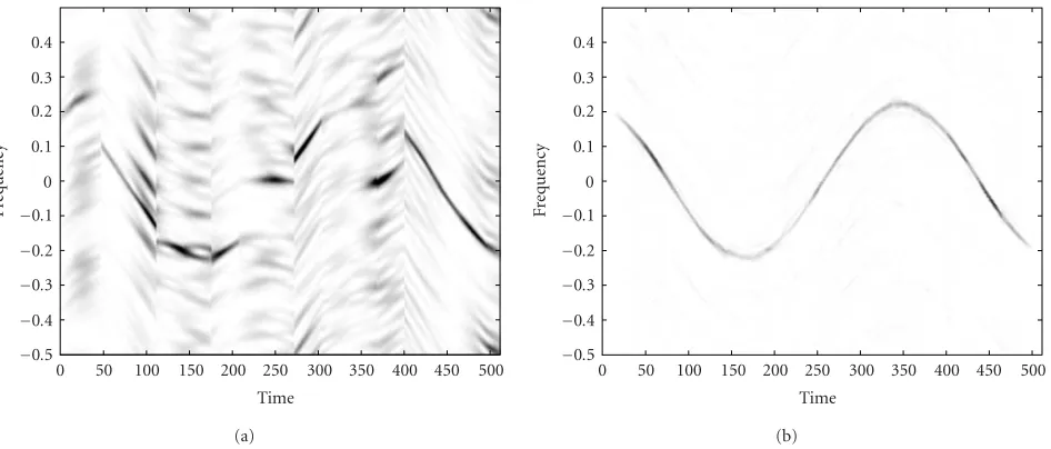
Figure4: The comparison between (a) MLPTFTpand (b) RMLPTFTpof a sinusoidal FM signal.
is high, the MSE is mainly affected by the bias which in-creases with the increase of window length. When SNR is low, the variance of the signal is the dominant factor af-fecting the MSE. The variances decrease with the increase of window length so that the MSE becomes relatively small. It is worth mentioning that, when SNR is extremely low, for example, below 0 dB, MSEs deteriorate significantly. This is because the windows used in our proposed MLPTFTp are generally with smaller length. The use of narrow win-dows leads to the increasing influence of noise especially for low SNR. The most important observation made in Figure 3 is that the MSE performances for different over-lap lengths are very close to each other regardless of the
window lengths, which leads to the conclusion that the de-crease of overlap length between segments does not dete-riorate the performance of MLPTFTp. In our investigation, several kinds of nonstationary signals, including the fourth-order polynomial phase signals, sinusoidal FM signals, and logarithm FM signals, have been used to reach similar con-clusions. Therefore, the reduction of computational com-plexity due to the reduction of the number of segments to be processed does not obviously deteriorate the MSE performance.
We now changew(t) embedded inx1(t) to be the impulse noise which belongs to the Middleton class A model [5,13] with the formw(t)=w1(t) +
40
0.4 0.3 0.2 0.1 0 −0.1 −0.2 −0.3 −0.4 −0.5
0 50 100 150 200 250 300 350 400 450 500 Time
Fre
q
u
en
cy
(a)
0.4 0.3 0.2 0.1 0 −0.1 −0.2 −0.3 −0.4 −0.5
0 50 100 150 200 250 300 350 400 450 500 Time
Fre
q
u
en
cy
(b)
Figure5: The comparison between MLPTFTpwith (a) fixed and (b) adaptive window length.
0.4 0.3 0.2 0.1 0 −0.1 −0.2 −0.3 −0.4 −0.5
0 50 100 150 200 250 300 350 400 450 500 Time
Fre
q
u
en
cy
(a)
0.4 0.3 0.2 0.1 0 −0.1 −0.2 −0.3 −0.4 −0.5
0 50 100 150 200 250 300 350 400 450 500 Time
Fre
q
u
en
cy
(b)
Figure6: Comparison between (a) MLPTFTpand (b) RMLPTFTpof the multicomponent signal with impulse noise.
10δ(t) andτiforms Poisson processes.Figure 4presents the MLPTFTpand RMLPTFTpto clearly show that good perfor-mance is achieved by using the RFT in RMLPTFTpinstead of the FT in MLPTFTp.
We consider the signal contains multiple components, which is defined as
x2(t)=exp
−j
256
π
cos
√
2πt
256
+ exp−j0.002πt2+exp−j0.002πt2+0.06πt
+w(t),
(15)
Figure 6shows the comparison between the MLPTFTp and RMLPTFTpwhenw(t)=0.9[w31(t) + jw32(t)]. The sig-nals(t) used is the same as in the previous experiment except that the third component is zero. The components smear sig-nificantly inFigure 6abecause the FT used in the MLPTFTp is not able to substantially suppress the non-Gaussian noise. However, the RMLPTFTp yields much better performance and the two components can be clearly seen inFigure 6b.
6. CONCLUSION
This paper presents analysis algorithms effectively dealing with time-varying multicomponent signals. In particular, these algorithms allow the reduction of computational com-plexity by minimizing the length of overlap between consec-utive signal segments. Experiments show that by using the proposed algorithms of parameters estimation and adaptive window length, the signals containing both single and mul-tiple components with Gaussian and impulse noises can be more accurately represented in the time-frequency domain.
REFERENCES
[1] S. Qian and D. P. Chen,Joint Time-Frequency Analysis: Meth-ods and Applications, Prentice-Hall, Upper Saddle River, NJ, USA, 1996.
[2] H. K. Kwok and D. L. Jones, “Improved instantaneous frequency estimation using an adaptive short-time Fourier transform,”IEEE Trans. Signal Processing, vol. 48, no. 10, pp. 2964–2972, 2000.
[3] V. Katkovnik, “A new form of the Fourier transform for time-varying frequency estimation,” Signal Processing, vol. 47, no. 2, pp. 187–200, 1995.
[4] I. Djurovic, “Robust adaptive local polynomial Fourier trans-form,”IEEE Signal Processing Lett., vol. 11, no. 2, pp. 201–204, 2004.
[5] D. Middleton, “Channel modeling and threshold signal pro-cessing in underwater acoustics: an analytical overview,”IEEE J. Oceanic Eng., vol. 12, no. 1, pp. 4–28, 1987.
[6] A. Scaglione and S. Barbarossa, “On the spectral properties of polynomial-phase signals,”IEEE Signal Processing Lett., vol. 5, no. 9, pp. 237–240, 1998.
[7] V. Katkovnik, “Robust M-periodogram,” IEEE Trans. Signal Processing, vol. 46, no. 11, pp. 3104–3109, 1998.
[8] I. Djurovic, V. Katkovnik, and L. J. Stankovic, “Median filter based realizations of the robust time-frequency distributions,” Signal Processing, vol. 81, no. 7, pp. 1771–1776, 2001. [9] V. Katkovnik, “Local polynomial periodograms for signals
with the time-varying frequency and amplitude,” inIEEE International Conference on Acoustics, Speech, and Signal Pro-cessing (ICASSP ’96), pp. 1399–1402, Atlanta, Ga , USA, May 1996.
[10] S. Peleg and B. Porat, “Estimation and classification of polynomial-phase signals,” IEEE Trans. Inform. Theory, vol. 37, no. 2, pp. 422–430, 1991.
[11] M. Z. Ikram and G. T. Zhou, “Estimation of multicomponent polynomial phase signals of mixed orders,” Signal Processing, vol. 81, no. 11, pp. 2293–2308, 2001.
[12] I. Djurovic, L. Stankovic, and J. F. Bohme, “Robust L-estimation based forms of signal transforms and time-frequency representations,”IEEE Trans. Signal Processing, vol. 51, no. 7, pp. 1753–1761, 2003.
[13] S. M. Zabin and H. V. Poor, “Efficient estimation of class A noise parameters via the EM algorithm,” IEEE Trans. Inform. Theory, vol. 37, no. 1, pp. 60–72, 1991.
Yongmei Wei received the B.E. degree in electronic and communication engineer-ing from Harbin Institute of Technology, China, in 2001. Now she is pursuing her Ph.D. degree in electrical and electronic en-gineering at Nanyang Technological Uni-versity, Singapore. Her current research in-terests include time-frequency analysis and its applications, interference excision, chan-nel estimation and adaptive modulation in communication systems.
Guoan Bireceived a B.S. degree in radio communications, from Dalian University of Technology, China, in 1982, an M.S. de-gree in telecommunication systems, and a Ph.D. degree in electronics systems, from Essex University, UK, in 1985 and 1988, re-spectively. Since 1991, he has been with the School of Electrical and Electronic Engi-neering, Nanyang Technological University, Singapore. His current research interests