Real-Time Optimal Trajectory Generation for Constrained Dynamical Systems

(1)

Constrained Dynamical Systems

Thesis by Mark B. Milam

In Partial Fulfillment of the Requirements for the Degree of

Doctor of Philosophy

California Institute of Technology Pasadena, California

2003

(2)

ii

c

° 2003 Mark B. Milam

(3)

(4)

iv

Acknowledgements

The work in this thesis would not of been possible without the help of many

in-dividuals. I would like to express my gratitude to Kudah Mushambi and Samuel

Chang for their contributions to the software package that resulted from this

re-search. I would like to acknowledge Simon Yeung, Jim Radford, Bill Dunbar,

Muruhan Rathinam, Michiel van Nieuwstadt, Sudipto Sur, and Francesco Bullo

for being generous with their time. Additionally, I would like to thank Youbin Mao

for the many invaluable discussions we have had over the years. Ryan Fran was

instrumental in getting the Caltech Ducted Fan experiment operational. I thank

him for his help on the experiment as well as introducing me to the sport of rock

climbing.

Prof. Nicholas Petit greatly influenced the work in this thesis. I would like to

thank him for his contributions to the micro-satellite project as well as evaluating

the performance of the proposed software algorithm in this thesis. I look forward to

collaborating with Nick in the future. My thanks go out to the dynamical systems

mavens: Wang Sang Koon and Prof. Jerrold Marsden provided the opportunity

to work on the micro-satellite project; Dong-Eui Chang for working with me on

the mathematical intricacies of differential flatness. I acknowledge Prof. Joel

Burdick for accepting to be a member of my thesis committee. Thanks to Prof.

John Hauser for contributing to the receding horizon control chapter of this thesis

as well as the design of the ducted fan experiment. I was surprised when we

met our goal of implementing receding horizon control on the experiment before

I graduated. I would like to reserve special acknowledgment for my mentor and

exemplary adviser, Prof. Richard Murray. Richard provided an unique

multi-discipline research environment as well as the inspiration, funding, guidance, and

motivation for my work.

I am indebted to Charmaine Boyd for handling the endless administrative

details of the Caltech ducted fan experiment. Thanks also to Rodney Rojas and

(5)

Rodney and I hoisted the 175 kg Caltech ducted fan experiment on its pedestal.

I owe gratitude to Northrop Grumman for providing a PhD fellowship to help

support my research.

I would like to thank to my parents, to whom I have dedicated this thesis,

for their support throughout the years. My wife, Joy, has always been loving

throughout this difficult experience while working full-time and raising our family.

She has always been my greatest source of energy to finish this thesis. For this, I

(6)

vi

Real-Time Optimal Trajectory Generation for Constrained

Dynamical Systems

by Mark B. Milam

In Partial Fulfillment of the

Requirements for the Degree of

Doctor of Philosophy

Abstract

With the advent of powerful computing and efficient computational algorithms,

real-time solutions to constrained optimal control problems are nearing a reality. In

this thesis, we develop a computationally efficient Nonlinear Trajectory Generation

(NTG) algorithm and describe its software implementation to solve, in real-time,

nonlinear optimal trajectory generation problems for constrained systems. NTG is

a nonlinear trajectory generation software package that combines nonlinear control

theory, B-spline basis functions, and nonlinear programming. We compare NTG

with other numerical optimal control problem solution techniques, such as direct

collocation, shooting, adjoints, and differential inclusions.

We demonstrate the performance of NTG on the Caltech Ducted Fan testbed.

Aggressive, constrained optimal control problems are solved in real-time for

hover-to-hover, forward flight, and terrain avoidance test cases. Real-time trajectory

generation results are shown for both the two-degree of freedom and receding

horizon control designs. Further experimental demonstration is provided with the

station-keeping, reconfiguration, and deconfiguration of micro-satellite formation

with complex nonlinear constraints. Successful application of NTG in these cases

demonstrates reliable real-time trajectory generation, even for highly nonlinear

and non-convex systems. The results are among the first to apply receding horizon

(7)

(8)

viii

List of Figures

1.1 Separation of different levels of trajectory generation. . . 2

1.2 Two-degree-of-freedom-design. . . 3

1.3 Receding horizon control design. . . 3

2.1 UCAV coordinate system conventions. . . 16

2.2 Ducted fan trajectory generation homotopy example: x: 0→ −.8 and z: 0→ −.8 with large time weight. . . 18

2.3 A flat system has the important property that the states and the inputs can be written in terms of the outputszand their derivatives. Thus, the behavior of the system is determined by the flat outputs. Note that the map wis bijective. . . 38

(12)

xii

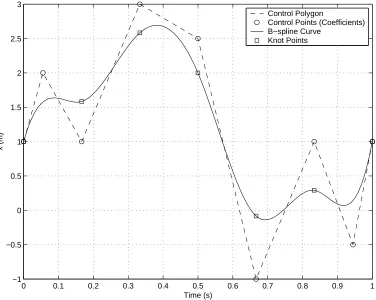
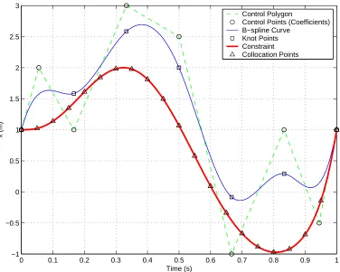
3.1 In this hypothetical problem, the B-spline curve has six intervals

(l = 6), fourth order (k = 4), and is C3 _{at the breakpoints (or} smoothness s = 3). The constraint on the B-spline curve (to be larger than the constraint in this example) will be enforced at the

21 collocation points. The nine control points are the decision

vari-ables. . . 60

4.1 RIOTS and NTG van der Pol comparison . . . 70

4.2 The different formulations of the optimal control problem for the

example. Top: full collocation. Bottom: flatness parametrization. . 78

4.3 Main results. The cpu-time is an exponential decreasing function

of the relative degree. Top: full collocation. Bottom: flatness

parametrization. . . 79

4.4 log(Number of variables) versus log(cpu-time). In each case 200

runs were done with random initial guesses. The variance of the results is represented by the error bar. The slope of the linear

regression of the mean values of cpu-time is 2.80 . . . 80 4.5 NTG direct collocation, “semi-flat” and “flat” convergence analysis.

The abscissa is the number of convergent test cases out of the 500

for each 6561 test case. The ordinate shows the number of 6561 test

cases. . . 83

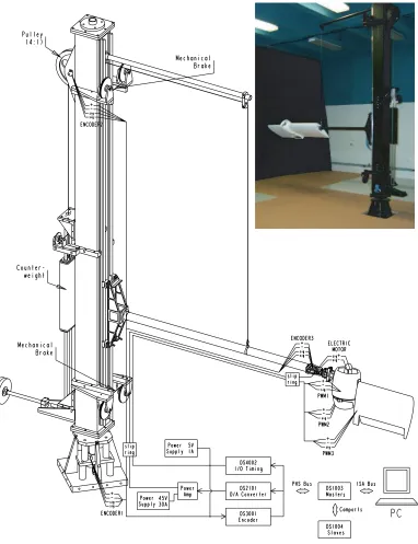
5.1 Ducted fan testbed . . . 87

5.2 Ducted fan coordinate frames . . . 88

5.3 B-spline curve fits to wind tunnel and flight test results for the

CL(α),CD(α), andCM(α) aerodynamic coefficients. . . 90 5.4 forward-flight mode equilibrium manifold . . . 93

5.5 Sample run showing joystick input and timing concepts. The initial

conditions for each run are denoted with IC, and the final conditions

(13)

5.6 “Shuttle” maneuver depicting joystick command , NTG reference

trajectory, and actual state . . . 97

5.7 “Shuttle” maneuver depicting all the trajectories that are computed and which trajectories are accepted. For each trajectory, a fixed constant is added to the time axis so that all trajectories can be seen. “X” denotes the start of a trajectory. “O” denotes an accepted trajectory that was applied until completion; that is, the system reached a hover equilibrium. . . 98

5.8 “Shuttle” Maneuver run times . . . 99

5.9 Terrain avoidance position and pitch attitude of the Caltech Ducted Fan. NTG reference trajectory (dashed) and actual (solid). The attitude (θ) is denoted by the orientation of the airfoil. . . 99

5.10 Terrain avoidance commanded and actual forces . . . 100

5.11 Hover to hover test case: Altitude and x position for two different vertical trajectory constraints. The actual (solid) and NTG ref-erence trajectories (dashed). The attitude (θ) is denoted by the orientation of the airfoil. . . 101

5.12 Forward-flight test case: θand ˙x desired and actual. . . 102

5.13 Forward-flight test case: Desired FXb and FZb with bounds. . . 103

5.14 Forward-flight accepted trajectory errors . . . 103

5.15 Forward-flight test case: Altitude andxposition (actual (solid) and desired(dashed)). Airfoil represents actual pitch angle (θ) of the ducted fan. . . 104

5.16 Forward-flight test case: 60 second run, 30 computed trajectories, tsample= 2 sec. . . 104

5.17 Illustration of sub-level set of J∗ T(·) to which the state of the true system will converge . . . 112

5.18 Illustration of timing scheme without prediction. . . 114

(14)

xiv

5.20 Plot depicting the actual attitude and position of the ducted fan

throughout both step commands. . . 119

5.21 The commanded forces in the body frame. There is a nonlinear transformation between FXB, FZB and commanded current to the motor and the thrust vector bucket angle δτ. . . 119

5.22 Horizontal position of the ducted fan . . . 120

5.23 The attitude of the ducted fan . . . 121

5.24 The spatial horizontal velocity of the ducted fan . . . 122

5.25 Force constraints and computation times. . . 123

5.26 Vertical position of the ducted fan . . . 125

6.1 Orbit and inertial coordinate systems. . . 132

6.2 Micro-satelllite modes of operation: reconfiguration, station-keeping, and deconfiguration . . . 134

6.3 Station keeping with guaranteed earth coverage . . . 136

6.4 Station-keeping for three micro-satellites. Relative distances (m) . 139 6.5 Station-keeping for three micro-satellites. Projected area (m2_{). . . 140}

6.6 Station-keeping for three micro-satellites. ∆V (m/s) . . . 141

6.7 Projected area for station-keeping with and without control. Pro-jected area (m2). Without control, the projected area becomes sin-gular. . . 142

6.8 Reconfiguration. Going into a formation with a projected area of 450m2. Top: projected area versus time. Middle: relative distances versus time. Bottom: thrusts in the body frame, where each colunm is a different satellite. . . 145

(15)

List of Tables

2.1 Summary of the flatness characteristics of several simple VTOL

con-figurations. Flat in forward flight implies that the mixing of hover

actuation and aerodynamic surfaces is possible. . . 46

4.1 Summary of results of simple cart comparison showing that

exploit-ing differential flatness compares favorably with other transcription

techniques. . . 68

4.2 RIOTS and NTG van der Pol comparison . . . 71

4.3 NTG Goddard example results showing the increase in accuracy in

solution as the number of knot intervals is increased . . . 73

5.1 Maximum acceptable periods as determined in simulation . . . 117

5.2 Maximum acceptable periods as determined on the real experiment 118

6.1 Station-keeping. Top: effect of S for a given d. Bottom: effect of e

(16)

1

Chapter 1

Introduction

A simple one-degree-of-freedom approach to tracking a real-time target using

feed-back control system is to subtract the current state of the system from the target

and feed this error to the controller. It is well known that this approach frequently

fails for a large class of nonlinear mechanical systems with constraints, where a

global asymptotically stable solution that satisfies the constraints does not exist.

Even when a solution is found, it is difficult to achieve high performance in the

presence of constraints.

When used in conjunction with a stabilization technique, generating a

trajec-tory that satisfies the system dynamics has been proven effective in mitigating the

deficiencies of the one-degree of freedom design. Typical applications of trajectory

generation include obstacle avoidance by a robotic vehicle, minimum time missile

interception of an agile target, formation flight of microsatellites with coverage

constraints, and a rapid change of attitude for an unmanned flight vehicle to evade

a dynamic threat. References [1] and [68] articulate the need for advanced control

techniques to accomplish these missions.

Depending on the system setup, there may be more than one level of trajectory

generation, as shown in Figure 1.1. At the mission level, an objective along with

a set of mission constraints are derived from high level mission inputs, with which

a desired trajectory is generated. The time-scale at this level of trajectory

(17)

(18)

1. Introduction 3

P

Plant ∆

Feedback

noise output

xd

Compensation ref

ud _u

δu

Trajectory Generation

Figure 1.2: Two-degree-of-freedom-design.

P

Plant ∆

output noise

ref Trajectory u Generation

Figure 1.3: Receding horizon control design.

controls of this trajectory are then applied for a certain fraction of the horizon

length, after which the process is repeated. It has been shown theoretically that

receding horizon control is stabilizing if an appropriate cost function is chosen and

the trajectory can be computed quickly.

It is possible to combine the two-degree-of-freedom and receding horizon control

designs. For example, one could generate a feasible trajectory using the

two-degree-of-freedom design and stabilize with the receding horizon control design.

A prime example, where a two-degree-of-freedom or receding horizon control

design would be applied, is an unmanned flight vehicle. The desired objective of the

unmanned flight vehicle could be commanded by the operator or pre-programmed

(19)

certain point, pass through several way-points, or track a target. For some

mis-sions, unmanned flight vehicles will autonomously fly highly aggressive maneuvers,

frequently on the fringe of the flight envelope. The idea of directly commanding

the unmanned flight vehicle to track a target would be impractical, considering

the fast dynamics and constraints of a typical unmanned flight vehicle. Some

fu-ture unmanned flight vehicles could autonomously launch an attack and return

to base or land on aircraft carriers. These vehicles would provide more tactical

flexibility than a cruise missile because they would be able to loiter in the area and

search for a moving target, which it could then strike with its weapons. Future

unmanned flight vehicles will have the ability to respond quickly to a wide range of

unforeseeable circumstances in search and rescue, border patrol, and counter-drug

operations. A key feature of these unmanned flight vehicles will be their ability to

autonomously plan their own trajectories. Therefore, the important goal of opti-mal trajectory generation is to construct, in real time, a solution that optimizes the

system objective while satisfying system dynamics, as well as state and actuation

constraints.

Hence, it is the objective of this thesis to develop an efficient computational

algorithm for real time optimal trajectory generation of constrained systems and

demonstrates its effectiveness on an experiment testbed that represents a

real-world application.

1.1

Previous and Parallel Work

Most early numerical methods of solution to constrained optimal trajectory

gener-ation problems relied on either indirect or direct methods of solution. The indirect

method relies on finding a solution to the Pontryagin’s maximum principle [83].

This results in finding a numerical solution to a two-point boundary value

prob-lem, if no closed form solution can be found. The multiple shooting method, used

to solve two-point boundary value problems, is discussed in Pesch [77, 78] and

(20)

1.1. Previous and Parallel Work 5 the objective function, subject to the constraints of the optimal control problem.

An introduction to direct methods can be found in Hargraves and Paris [41] and

vonStryk [109]. Techniques were developed to optimally interpolate a set of stored

trajectories on-line by Chen and Allgower in [18] and [3], respectively. A

tech-nique for generating real time trajectories by searching and interpolating over a

large trajectory database in real time can be found in Atkeson [4].

Several randomized trajectory generation techniques have recently been

re-ported and have promising potential for real-time applications. For example, see

LaValle [55], Frazzoli [36], and Hsu [44]. These techniques are most applicable to

the mission level trajectory generation shown in Figure 1.1.

Another approach to solving the trajectory generation problem would be to use

nonlinear geometric control techniques. These techniques attempt to find ad hoc

outputs such that the complete differential behavior of the system can be

repre-sented in terms of these outputs and their derivatives. The theory of existence and

generation of these so-called flat outputs are subjects of Isidori [46], Rathinam [87],

Charlet et al. [16], Fliess [32, 33], Chetverikov, [19], and [62, 65]. Unfortunately, there are many classes of systems for which these outputs cannot be found, even

if they can be proven to exist. However, it is usually not very difficult to find

some outputs that will characterize at least part of the system behavior. In this

case, attention must be paid to the stability of the resulting zero dynamics which

could lead to unbounded controls and states. Techniques were developed in

Deva-sia and Chen [25], DevaDeva-sia [24], and Verma and Junkins [107] to circumvent this

problem. Some methods of real-time trajectory generation without constraints for

differentially flat systems are illustrated in van Nieuwstadt [103]. An approach to

find feasible trajectories for constrained differentially flat systems by

approximat-ing constraints with linear functions is given in Faiz and Agrawal [29]. Agrawal

and Faiz in [2] investigated higher-order variation methods to solve optimization

problems for feedback linearizable systems without constraints.

An example of work more related to the approach in this thesis can be found in

(21)

quadratic programming can drastically reduce computation times in robotic

mo-tion planning. The work of Oldenburg et al. [75] and [76] expands on Steinbach’s approach by including the case when the system is not feedback linearizable.

Old-enburg relies on the work of van der Schaft in [102], which provides a method to

represent a nonlinear state space system as a set of higher-order differential

equa-tions in the inputs and outputs. Mahadevanet al. in [60] and [61] use Oldenburg’s work and apply it to chemical processes. Veeraklaew et al. in [106] combines the concepts of differential flatness and sequential quadratic programming. However,

his choice of basis functions representing the outputs requires additional continuity

constraints to the resulting optimization problem. Bulirschet al. [37] discusses the use of sequential quadratic programming methods to solve trajectory optimization

problems.

1.2

Overview and Statement of Contributions

A brief summary and thesis contributions by chapter:

• Chapter 2: In this chapter we derive a novel homotopy method, which when used in conjunction with a stored database of trajectories, will find nearby

optimal trajectories. Additionally, we discuss the relationships between

Ver-tical Takeoff and Landing (VTOL) design and differential flatness. Finally,

we present a promising new VTOL design and demonstrate that it is

differ-entially flat.

• Chapter 3: In this chapter we first propose a generic algorithm to reduce the dimension of the system dynamics to facilitate real-time computation.

Sec-ond, we develop the Nonlinear Trajectory Generation (NTG) algorithm and

describe the software implementation intended to solve nonlinear, optimal,

real-time, constrained trajectory generation problems. NTG is a software

package that combines techniques of nonlinear control, B-splines, and

(22)

1.2. Overview and Statement of Contributions 7 • Chapter 4: In this chapter, we compare and contrast NTG with the optimal control problem solution techniques of direct collocation, shooting, adjoints,

and differential inclusions.

• Chapter 5: In this chapter, we investigate the performance of NTG on the Caltech Ducted Fan experiment. Results are presented for both the

two-degree-of-freedom and receding horizon control design. For the two-degree

of freedom design, aggressive constrained optimization problems are solved in

real-time for hover-to-hover, forward flight, and terrain avoidance test cases.

The results confirm the applicability of real-time, nonlinear, constrained

re-ceding horizon control. They are among the first to demonstrate the use

of receding horizon control for agile flight in an experimental setting, using

representative dynamics and computation.

• Chapter 6: In this chapter, we provide another example of complex, real-time nonlinear constrained trajectory generation for the station-keeping,

(23)

Chapter 2

Background and Mathematical Framework

In this chapter we will survey the techniques that are currently used for

con-strained trajectory generation, followed by background material that motivates

this research.

2.1

Optimal Control Problems under Consideration

Letx: [t0, tf]→Rndenote the state of the system and u: [t0, tf]→Rmthe input of the system

˙

x=f(x, u), (2.1)

where all vector fields and functions are real-analytic. It is desired to find a

tra-jectory of (2.1) in [t0, tf] that minimizes the performance index functional

J := Z tf

t0

L(x, u, t)dt+φf(xf, uf, tf) (2.2)

J : Rm×R+ → R subject to a vector of N0 initial time, Nf final time, and Nt trajectory constraints,

lb0 ≤ ψ0(x0, u0)≤ub0,

lbf ≤ ψf(xf, uf)≤ubf,

lbt ≤ S(x, u, t)≤ubt.

(24)

2.2. Necessary Conditions of Optimality for Constrained Systems 9 The functionsψ0 :Rn×Rm →RN0,ψf :Rn×Rm →RNf,S:Rn×Rm×R+→

RNt _{are assumed to be as least} _C2 _{on appropriate dense open sets. The final time}

tf could be either fixed or free.

2.2

Necessary Conditions of Optimality for Constrained

Systems

Bryson and Ho [12] and Lewis and Syrmos [58] derive the necessary conditions

using the calculus of variations. Pontryagin et al. [83] show that finding an ex-tremal solution is equivalent to the requirement that the variational Hamiltonian

be minimized, with respect to all admissible inputs.

Without loss of generality, we will assume that there is one control (m = 1) and one state inequality constraint (Nt = 1, S(x, t) ≤ 0) and that the trajectory constraint is active on the time interval t∈[t1, t2]⊂[t0, tf]. An active constraint is known as a constrained arc.

Defining the HamiltonianH and the auxiliary functions Ξ and Φ,

H(x, u, λ, µ, t) :=L(x, u, t) +λT_f₍_{x, u}_{) +}_µT_S(q)₍_{x, u, t}₎ Ξ(x0, u0, t0, ν0) :=φ0(x0, u0, t0) +ν0Tψ0(x0, u0, t0) Φ(xf, uf, tf, νf) :=φf(xf, uf, tf) +νfTψf(xf, uf, tf),

(2.4)

where the λ : [t0, tf] → Rn, ν0 ∈ RN0, νf ∈ RNf and µ : [t0, tf] → R are La-grange multipliers. The number of time derivatives q of S such that u explicitly appears and Su(q)6= 0 is denoted byS(q)(x, u, t). In order thatS(q)(x, u, t) = 0 and

S(x, u, t) = 0 on [t1, t2] we also require that the entry conditions

NT(x(t1), t1) = [S(x(t1), t1), S(1)(x(t1), t1), . . . , S(q−1)(x(t1), t1)] = 0 (2.5)

be satisfied. See Bryson, Denham and Dreyfus [11] for more details. The Lagrange

(25)

An optimal solution of (2.2) and (2.3) must satisfy the the necessary conditions

˙

x=Hλ (2.6)

˙

λT =−Hx (2.7)

Hu = 0 (2.8)

λT(t0) = Ξx|t=t0 (2.9)

λT(t−₁) =λT(t+₁) +πTNx|t=t₁ (2.10)

H(t−₁) =H(t+₁)−πTNt|t=t₁ (2.11)

λT(tf) = Φx|t=tf (2.12)

µ= 0 if S(q)(x, u, t)<0 (2.13)

µ≥0 if S(q)(x, u, t) = 0 (2.14)

and if the final time tf is not specified we must include

(Φt+H)|t_f = 0. (2.15)

Note: The partial derivativesHx, Ξx, and Φx are considered row vectors, i.e.,

Hx= (_∂x∂H₁, . . . ,_∂x∂H_n) and the transpose of the column vector (.) is denoted by (.)T The necessary conditions result in a multi-point boundary value problem at

times t0, t1 and tf involving the differential equations (2.6) and (2.7). At each boundary there will be effectivelyn constraints derived from the total number of terminal equations minus the free variables.

Utilizing (2.11) and (2.15), we can determine t1 and tf. The input on the constrained arc can be found fromS(q)(x, u, t) = 0. Otherwise we can use equation (2.8). The Lagrange multiplier µis found from equation (2.13) off the constrained arc and equation (2.8) when on the constrained arc.

Generally, closed form solutions are difficult to find. Numerical methods based

on gradient descent or Newton’s method are usually invoked to find solutions to

(26)

2.3. Trajectory Generation Using Homotopy 11 guess to the free-variables ν0, νf, π, t1, and tf sufficiently close to a solution to guarantee convergence of the method.

The multiple shooting numerical method is advocated by Pesch in [77] and [78].

A thorough description of shooting techniques is provided by Stoer and Burlisch

[99]. One advantage of using shooting is that very accurate solutions are

obtain-able. Potential disadvantages of shooting include a high sensitivity to the initial

guess, as well as the need for robust integration techniques over large time intervals

since equations (2.6) and (2.7) will likely have both unstable and stable

compo-nents. An alternative to the shooting method, which is less sensitive to the initial

guess, is to replace the ordinary differential equations in equations (2.6) and (2.7)

by their finite difference approximations. Press et al. discuss so called relaxation methods solution methods in [86]. Due to the undesirable convergence rates and computation times, neither of these numerical methods are practical for real-time

implementation. In the next section, we will assume that a solution to an optimal

control problem can be determined off-line using the above mentioned numerical

techniques and stored in a database for on-line use. We will use a trajectory in the

database as the initial guess to solve a neighboring optimal control problem with

high confidence in real-time.

2.3

Trajectory Generation Using Homotopy

Homotopy can best be shown by a simple example. Suppose that one wishes to

obtain the solution of a system ofN nonlinear equations inN variables,

W(x) = 0, (2.16)

where W : RN → RN is a smooth mapping. Without a good initial guess ¯x, an iterative solution to equation (2.16) will often fail. As a possible remedy, one

defines a homotopy V :RN×R→RN such that

(27)

whereU :RN _→_RN _{is a smooth map having known solutions. Typically, one may} choose a convex homotopy such that

W(x, ²) :=²U(x) + (1−²)V(x),

and continuously trace an implicitly defined curve from a starting point (x1,1) to a solution (¯x,0). Burlisch in [13] and [99] warns that morphing a simple system not related to the problem to a complex system may not succeed in critical cases.

In the following section, a homotopy method is presented without applying a

homotopy to the system dynamics. Chenet al. [18] also took a similar approach to singular optimal control problems.

2.3.1 Algorithm Description

It will be assumed that the desired objective is to move the system from a known

initial state to a known final state while minimizing a prescribed cost function.

The proposed homotopy algorithm will find an optimal trajectory connecting the

initial and final state. The central idea of the algorithm is to decompose the

operating envelope into regions. For each region a trajectory is computed off-line

and the initial and final states and costates are saved into a database for on-line

use. The boundaries of each region are determined such that for each trajectory

in the region, there exists a homotopy to any other trajectory in the region. The

advantages to this algorithm is that only a small subset of all trajectories need to

be stored on-board, and every trajectory is optimal with respect to a prescribed

cost function.

We tacitly assume that a solution has been found to the trajectory generation

problem for some specified system (2.1), with associated cost function in equation

(2.2), an initial state constraint ψ0(x0) = 0, and the desired state ψf(xf) = 0. A solution to this problem implies that we have also foundν0andνf in equation (2.4). Now suppose that we would like to determine the solution with the new boundary

(28)

2.3. Trajectory Generation Using Homotopy 13 tox(t0) andψ(x(tf)) = 0, respectively. By “sufficiently close” we mean that there exists a homotopy between x(t0) and ψ(x(tf)) = 0 and ˜x(t0) and ˜ψ(x(tf)). The implicit function theorem will dictate whether or not a homotopy exists. To obtain

a solution with the new desired goal ˜ψ(x(tf)) and initial state ˜x(t0), we will embed the known solution into a family of perturbed solutions through the parameter ²

using a convex homotopy. Define

ˆ

x(t0, ²) := x(t0)²+ ˜x(t0)(1−²) (2.17) ˆ

ψ(x(tf), ²) := ψ(x(tf))²+ ˜ψ(x(tf))(1−²), (2.18)

where ² ∈ [0,1] is a perturbation parameter, ˆx(t0, ²) : Rn ×[0,1] → Rn, ˆψ :

Rn_×_[0_,_1]_→_Rp_{. By making}_²_{go to zero, we obtain the solution to the trajectory} generation problem of interest.

In principle, we know that the solutions of the differential equations (2.6) and

(2.7) are determined by x(t0) andλ(t0). That is, if we alterψ0 and ν0, we change

x and λfor allt. Thus, we may write at the final time tf:

x(tf) =x(ψ0, ν0, tf) λ(tf) =λ(ψ0, ν0, tf). (2.19)

For ease of notation, we will write the terminal boundary conditions as

G(y, ²) = 0, (2.20)

wherey = (ν0, νf) and Gis an (n +N0) vector-valued functional.

Suppose we are given a solution (z0, ²0) of (2.20). Using homotopy, we want to find a solution z(²0+ ∆²) for a small perturbation ∆². The implicit function theorem [50] gives conditions which one can solve (2.20) in some neighborhood of

(z0, ²0):

a. G(z0, ²0) = 0 for some z0 and ²0; b. Gz(z0, ²0) is nonsingular;

(29)

(30)

2.3. Trajectory Generation Using Homotopy 15 Changingz, while holding²constant, we have _∂x∂x

0(t0) = 0∈R

n×n_,∂λ

∂λ0 =I6∈

Rn×n_, ∂x

∂λ0 = 0 ∈ R

n×n_{, and} ∂λ

∂x0 = 0 ∈ R

n×n _{. Now we can find} _G

z(z, ²) by integrating theη(t) and ξ(t) dynamics forward in time:

Gz(z, ²) =Gz(η(tf), ξ(tf), ²). (2.24)

In an analogous manner, the following differential equations are derived which

we will use to calculate the Jacobian G²(z, ²) (holdingz0 constant). Defining

ζ = ∂x

∂², χ= ∂λ

∂², ζ, χ∈R

n

we obtain

˙

ζ =Hλx·ζ+Hλλ·χ+Hλ² (2.25) ˙

χ=Hxx·ζ+Hxλ·χ+Hx² (2.26)

and observe that if we change², but holdzconstant, we have, referring to equation (2.17),ζ(t0) =x(t0)−x˜(t0) andχ(t0) = 0. Now we can findG²(z, ²) by integrating theζ(t) and χ(t) dynamics forward in time:

G²(z, ²) =G²(ζ(tf), χ(tf), ²). (2.27)

2.3.2 Ducted Fan Example

An example of the use of the homotopy technique will be illustrated using the

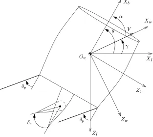
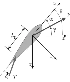
planar ducted fan. Figure 2.1 depicts the coordinate systems and conventions

used for the ducted fan. Writing Newton’s equations about Ow we have

mx¨ = FXbcosθ+FZbsinθ (2.28)

mz¨ = −FXbsinθ+FZbcosθ+mg (2.29)

(31)

The numerical values of the constants used in this example are the following:

m= 2.2kg mg= 4N rp =.2m J = 0.05kgm2. (2.31)

The optimal cost with free final time is

min u J ≡

Z T 0

(RT +R1FX2b+R2F

2

Zb)dt, (2.32)

with input constraints−5≤FZb ≤5 N, 0≤FXb ≤17 N, as well as constraints on

the initial and final state. The problem can be described as the following: Minimize

a balance between time and energy subject to initial and final time constraints as

well as a trajectory constraint on the input.

δe

Ow

Zb

Zw

γ

Xw

α

θ V

Xb

δp

XI

ZI

Figure 2.1: UCAV coordinate system conventions.

In this example, the integration technique used was a predictor-corrector

(32)

2.3. Trajectory Generation Using Homotopy 17 For the first example we computed off-line a trajectory using the optimal

tra-jectory solver RIOTS [90] for the initial conditions x(t0) = (0 0 0 0 π/2 0)T and the final conditions ˆψ(x(tf)) = ψ(x(tf)) =x(tf)−(1 0 −1 0π/2 0)T. The cost function weights were chosen as RT = 4, R1 = 1, and R2 = 2. It is desired to deform the initial condition to ˜x(t0) = (−1 0 −1 0π/2 0)T. Note that the final unknown time is a free variable. The predictor-corrector algorithm was coded in

Matlab and consumed approximately 11 minutes of CPU time on a Sun Ultra 30.

The results of the simulation showed that the homotopy could be performed, but

the computation time was prohibitive.

The same setup was used for the second example, except that RT = 200 and ˜

x(t0) = (−.8 0 −.8 0π/2 0)T. The difference between the two examples is that, in the second, there is significant weight on the time. The results of this simulation

are shown in Figure 2.2. For this example, it took approximately 38 minutes of

CPU time.

At ² = .35 the trajectory suddenly changes. This can be explained by the significant positive to negative change of Lagrange multiplier λ3(t0). The sign of the determinant ofGz(z, ²) indicates a singularity. However, the implementation of the algorithm is robust enough so that we still proceed with the homotopy in effect,

jumping over the singularity. Note that this singularity is not explicitly occurring

the the time domain since the homotopy parameter does not enter explicitly in the

state or costate equations. It is the significant change inλ3(t0) that is causing the large change in the dynamical behavior seen in Figure 2.2.

The unexpected singularity illustrates the necessity of an off-line study to find

trajectories such that we can steer around singularities. The nonsingularity of

det(Gz(z, ²)) 6= 0 must be off-line. If a singularity occurred, a modification of the cost function would be of first consideration. If a modification of the cost

function does not work, one could break the problem into separate homotopy

problems: x(t0) → x¯(t0) and ψ(x(tf)) → ψ¯(x(tf)) and then ¯x(t0) → xˆ(t0) and ¯

(33)

(34)

2.4. Nonlinear Programming Techniques 19 would be a last resort.

In general, another fundamental problem with this technique is sensitivity. We

are using a form of shooting to find Gz(z, ²) by integrating a system of ordinary differential equation that have both stable and unstable components. Integrating

such a system of ODE’s over a significant time span can become ill-conditioned.

This results in the ODE solver proceeding very slowly, producing large CPU times.

This sensitivity is due the nature of the necessary conditions of optimal control.

Multiple shooting may help mitigate some of these integration problems.

2.4

Nonlinear Programming Techniques

The problem of finding a local minimizer x ∈ Rn _{for a nonlinear function} _F₍_x₎ subject to a set of nonlinear constraints c ≥ 0, where c(x) ∈ _Rn_{, is a} _nonlinear

constrained optimization problem. All the problems of interest to be solved in this thesis can be generalized into the form

min x F(x)

subject to c(x)≥0.

(2.33)

Optimization problems of the form (2.33) can be a very difficult problem to solve.

For instance, it is NP-hard in the traditional complexity model [105]. Algorithms

to solve (2.33) may take many iterations and function evaluations. A promising

global optimization technique, based on surrogate functions, is given by Denniset al. [23]. Global optimization of (2.33) is a difficult problem and an open area of reserach . In this thesis, we will concentrate on using the well understood numerical

techniques that will find local minima of (2.33).

Sequential Quadratic Programming (SQP)and Interior Point Methods (IPM)

are popular classes of methods considered to be effective and reliable method for

locally solving Equation (2.33). At each iteration of an SQP method, one solves

a quadratic program (QP) subproblem that models (2.33) locally at the current

(35)

next iterate. Eliminating inequality constraints by adding slack variables and

incorporating them into a logarithmic barrier function in the objective function,

(2.33) is transformed into

min

x F(x)−µ m X i=1

logsi

subject to c(x)−s= 0.

(2.34)

Interior point refers to the fact that the slack variables are required to remain

strictly positive throughout the optimization.

Successful algorithms need to be both efficient and robust. Under reasonable

assumptions, a robust algorithm must be globally convergent (convergent from

any starting point) and able to solve, in practice, both well-conditioned and

ill-conditioned problems. NPSOL [38], SNOPT [39], CFSQP [57], KNITRO [110],

and LOQO [104] are the nonlinear programming solvers we consider in this thesis.

2.4.1 Optimality Conditions

Definition 2.1. A pointx∗ _{is a local minimizer of (2.33) if}

1. c(x∗₎_≥_0;

2. there exists a δ >0 such that F(x)> F(x∗_{) for all}_x _satisfying

||x−x∗|| ≤δ and c(x)≥0.

The termactive constraint will be used to designate a constraint ci(x)≥ 0 if

ci(x) = 0. If ci(x)>0, a constraint is consideredinactive.

The LagrangianL(x, λ)≡F(x)−λTc(x) is a scalar function with then vari-ablesx and the mvariables λwhich correspond to the Lagrange multipliers. The Lagrangian is used to express first-order and second-order optimality conditions

for a local minimizer.

(36)

con-2.4. Nonlinear Programming Techniques 21 straint qualification ensures the existence of the Lagrange multipliers. One such

constraint qualification is that the gradients of the active constraints atx∗ _be

lin-ear independent, i.e., that matrix ˆJ(x∗_{) should have full row rank. A point that}

satisfies this particular constraint qualification is known as a regular point. Necessary conditions forx∗_{to be a local minimizer are that there exist Lagrange}

multipliers λ∗ _{such that}

c(x∗)≥0 (2.35)

∇xL(x∗, λ∗) =∇F(x∗)−Jˆ(x∗)Tλ∗= 0 (2.36)

λ∗≥0. (2.37)

These conditions are known as thefirst-order Karush-Kuhn-Tucker (KKT) neces-sary optimality conditions. Note that x∗ _{is a stationary point of} _∇x(_x∗_{, λ}∗_{) but}

not necessarily an unconstrained minimizer of the Lagrangian.

Suppose that x∗ _{is a local minimizer and a regular point. Then,} _x∗ _{is a KKT}

point and

ZT∇2_xxL(x∗, λ∗)Z is positive semidefinite, (2.38)

where Z is a basis for the nullspace of ˆJ. These conditions are known as the

second-order KKT conditions. If we replace (2.37) and (2.38) by

λ∗ _>₀

ZT∇2xxL(x∗, λ∗)Z is positive definite,

(2.39)

we obtain sufficient conditions for optimality.

A key challenge to developing a fast algorithm for solving this problem is to

find an accurate approximation to the Hessian of the Lagrangian ∇2

xxL(x, λ), the second derivative that reflects the curvature of the objective and constraints.

The common approach to approximating∇2

xxL(x, λ) has been to follow quasi-Newton techniques for unconstrained optimization. A single, positive-definite

(37)

(BFGS)quasi-Newton update, and typically the dependence of the Lagrange mul-tipliers is ignored. See Gill et al. [40] for a complete discussion on the BFGS method. The BFGS direct approximation may be poor, even for ideal problems,

but has been used in CFSQP and NPSOL successfully. KNITRO and LOQO use

analytical Hessians of the constraint and objective to form the approximation to

the Hessian of the Lagrangian.

2.4.2 Techniques for Global Convergence

Nearly all techniques for nonlinear programming are iterative, producing a

se-quence of subproblems related in some way to the original problem. Newton

methods have rapid local convergence rates, but fail to converge from all

start-ing points. Gradient descent methods converge from nearly any startstart-ing point but

have poor local convergence properties. Line-Search methods are one means of ensuring global convergence while attempting to maintain fast local convergence.

Line-Search methods limit the size of the step taken from the current point to the

next iterate. Such methods generate a sequence of iterates of the form

xk+1 =xk+αp,

wherep is the search direction obtained from the subproblem, and α is a positive scalar steplength. For unconstrained minimization, or if feasibility is maintained for the constraints as with CFSQP, the best steplength is one that minimizes

the objective function F(xk+1). However, determining a minimizer along p is an iterative process and frequently time consuming. Typically, x is determined by a finite process that ensures a reduction inF(x). The nonlinear programming code NPSOL and LOQO use line-search methods. See Fletcher [31] for an overview of

(38)

2.4. Nonlinear Programming Techniques 23

2.4.3 Trust-Region Methods

The main alternative to line-search methods aretrust-region methods. The moti-vation behind the trust-region approach is that the minimum of the local quadratic

model should be accepted so long as the model adequately reflects the behavior

of the function under consideration. Trust-region methods choose a radius δ and determine xk+1 that is the global minimizer of a model of the function subject to ||xk+1−xk|| ≤ δ. The nonlinear programming code KNITRO uses trust region methods.

2.4.4 Merit Functions

Regardless of whether a line-search or trust-region method is used, when

feasi-bility of the iterates is not maintained, it can be difficult to guide the choice of

steplength. For problems with linear constraints, it is straightforward to maintain

feasibility at every iteration. However, when even a single constraint is nonlinear,

maintaining feasibility at every iteration becomes difficult. For infeasible iterates,

it is not immediately obvious how to choose the step length; we would like the next

iterate to minimize the objective function, but we would also like to reduce the

in-feasibilities of the constraints. Merit functions are used to guide the improvement

of the feasibility and the optimum at the same time. Since NPSOL, LOQO, and

KNITRO use merit functions, they are considered infeasible methods. CFSQP is

a feasible method; thus, there is no need for a merit function. If we assume, for

simplicity that all constraints are equalities of the form c(x) = 0, two popular merit functions are the l1 merit function

M(x) =F(x) +ρ||c(x)||1

and the augmented Lagrangian

M(x, λ) =F(x)−λTc(x) +ρ 2c(x)

(39)

(40)

2.5. Numerical Solutions of Optimal Control Problems Using Nonlinear Programming25 Similarly, NPSOL solves quadratic program

min p g(x0)

T_p₊1 2p

T_∇2

xxL(x0, λ0)p (2.41) subject to G(x0)p−c(x0) = 0. (2.42)

2.4.6 Active Set Methods

The active set method starts with a feasible pointp0and a working set of variables. The active set method proceeds to move to a constrained stationary point of the QP

by holding a set of variables constant and temporarily ignoring the other bounds.

If the solution (the new search direction p) to the QP program (2.42) is feasible with respect to the bounds, a full step is taken. Otherwise, the maximum feasible

step is taken along the search direction and a bound is added to the working set.

This sequence repeats until a full step is taken. At the stationary point, if for any

bound there exists a negative Lagrange multiplier, the associate bound is dropped

from the working set and the procedure starts over. If all the multipliers are

positive, the algorithm stops. NPSOL and CFSQP are active set methods.

It looks promising that interior point methods may show a significant reduction

in the total number of iterations compared to active set methods. The subproblem

may take longer than any one QP subproblem computation, but the time of this

one iteration will be faster than the total QP computational time. Active set methods take a combinatorial number of iterations for the subproblem.

2.5

Numerical Solutions of Optimal Control Problems

Using Nonlinear Programming

2.5.1 Direct Methods of Solution Using Nonlinear Programming

We can deduce from Section 2.2 that the trajectory generation problem can be

formulated in terms of an optimal control problem. In general, the optimal control

(41)

Indirect methods are based on the calculus of variations and the maximum

principle. In the direct approach, the optimal control problem is transformed into

a nonlinear programming problem (NLP). In Section 2.2 an indirect method was

used to solve the optimal control problem. For an overview of the indirect and

direct methods see Betts [7, 5] and Stryk and Burlisch [109]. In this section we

will concentrate on the direct method of solution.

Direct methods are generally more robust to the initial solution guess than

indirect methods. This is a result of not having to explicitly solve the necessary

conditions of optimal control, which are frequently ill-conditioned. In addition,

unlike indirect methods, direct methods do not require an a priori specification of

the switching structure when inequality state constraints are present. However, it

appears that the computational requirements of direct methods are at least that

of indirect methods.

The collocation method of [42] and adjoint method [82] are the methods of

transcription that are most relevant to the trajectory generation problem.

Se-quential quadratic programming, presented in Gillet al( [40] and [56]et al.,is the technique we will use to solve the nonlinear programming problems presented in

this thesis.

The nonlinear programming problem can be stated as the following:

min y∈RMF(y)

subject tolj ≤cj(y)≤uj j= 1, . . . , mN,

(2.43)

where lj and uj ∈ R,the constraint function cj : Rn → R is at least C2, and the cost function F :Rn _→ _R _{is also at least} _C2_{. We will rely on commercially} available nonlinear programming packages. It will be required that the nonlinear

programming problem be provided, not only the cost function and the constraints,

but also gradients of cost function and constraints with respect to the decision

variables y.

(42)

2.5. Numerical Solutions of Optimal Control Problems Using Nonlinear Programming27 optimal control problem to the nonlinear programming problem.

2.5.2 Transcription Techniques from the Optimal Control

Prob-lem to the Nonlinear Programming ProbProb-lem

Collocation

A reliable method to convert an optimal control problem to a nonlinear

program-ming problem is collocation. For an overview of collocation methods see Stryk

[108].

The first step in collocation process is to break the time domain into smaller

intervals

t0 < t1 < . . . < tN =tf. (2.44)

The nonlinear programming decision variables then become the values of the state

and the control at the grid points, namely,

y= (u0, x1, u1, x2, u2, . . . , xN, uN). (2.45)

The key notion of collocation methods is to replace the original system in equation

(2.1) with a set of defect constraintsζi = 0, which are imposed on each interval of discretization. An expression ofζican be derived based on the choice of numerical integration.

If we assume, for illustration, that there is also a state variable equality

(43)

(44)

(45)

constraints and trajectory equality constraints, can be found in a similar manner.

Once the gradients are known, there is enough information to solve the nonlinear

programming problems in (2.43).

2.6

Trajectory Generation Using Feedback

Lineariza-tion

The system under consideration in this section is

˙

x=f(x) +g(x)u y =h(x)

(2.51)

x ∈ Rn_, _u _∈ _Rm_, _y _∈ _Rm_{. The non-affine system in equation (2.1) can be} transformed into this form by adding integrators to all inputs.

2.6.1 Mathematical Background

We define adfgj = [f, gj] as the Lie Bracket of the smooth vector fields f and gj and

[f, g] = ∂g

∂xf − ∂f

∂xg=Lgf −Lfg.

where gj is the jth column of g(x) in equation (2.51). We note that ad0f =g and adk

fg= [f,adkf−1g] for all k≥1. Define the distributions

∆0 = span{gj,1≤j≤m}

∆i = span{adi_fgj,0≤l≤i, 1≤j≤m} i >0,

which have the recursion properties

∆i+1 = ∆i= adi+1f ∆0= ∆i+ adf∆i

(46)

2.6. Trajectory Generation Using Feedback Linearization 31 The Lie derivative of a functionh with respect to a vector fieldf

Lfh=

∂h

∂xf (2.52)

is the scalar function corresponding to the directional derivative of h along the direction off. Thek-th Lie derivative of hwith respect tof is defined recursively by the function

Lk_fh=LfLk_f−1h. (2.53)

A distribution ∆ is involutive if and only if, given any pair of vector fieldsg1 and g2 in ∆, their Lie Bracket [g1, g2] belongs to ∆.

2.6.2 Classical Feedback Linearization

We will make use of the notion of observability in the sequel. A system 2.51 is

said to be observable if

Theorem 2.1. Observability (Sontag [97])

dim(Span(h1, adfh1, . . . , adkf1−1h1, . . . ,(hm, adfhm, . . . , adfkm−1hm)) =n

for some ki such thatPm₁₌₁ki =n.

Definition 2.2 (Feedback linearizability). The nonlinear system in (2.51) is

feedback linearizable if there is a dynamic feedback

˙

z=α(x, z, v) z∈Rp

u=β(x, z, v) v∈Rm

(2.54)

and new coordinatesξ =φ(x, z) andη=ψ(x, z, v) such that in the new coordinates the system has the form

˙

ξ =Aξ+Bη, (2.55)

(47)

(48)

(49)

1. ∆i is an involutive distribution of constant rank for everyi≥0; 2. rank∆n−1 =n.

Remark 2.1. The theorem implies that there exists outputs λ1(x), . . . , λm(x) such that, relative to the outputs λi the system has Pri = nin a neighborhood or the origin. The functions λ1(x), . . . , λm(x) can be constructed by solving a set of first order partial differential equations of the form

LgjL

k

fλi(x) = 0 for all 0≤k≤ri−1,1≤j≤m.

It has been shown by Charlet et al. in [16] that (2.51) with m = 1 local static feedback linearization is equivalent to dynamic feedback linearization. For

m > 1, necessary and sufficient conditions do not exist for dynamic feedback linearization. Thus, the difficulty of finding linearizing outputs for

multi-input-multi-output systems is compounded by the fact that the system may not be

static feedback linearizable, but still dynamically feedback linearizable.

Example 2.1. Consider the dynamics of the planar ducted fan shown in Figure 2.1 with unity mass, inertia, distance from the center of mass to theFZbapplication

point, and gravitational force.

¨

x = FXbcosθ+FZbsinθ (2.62)

¨

z = −FXbsinθ+FZbcosθ+ 1 (2.63)

¨

θ = FZb. (2.64)

Choosing outputs to be

(50)

(51)

essentially a dynamic feedback of the form (2.54), but with the added requirement

that the compensator can be uniquely determined as function of x, u and a finite number of derivatives ofu. They have shown that dynamic feedback linearization via endogenous feedback is equivalent to differential flatness.

2.6.3 Devasia-Chen-Paden Non-minimum Phase Zero-Dynamics

Algorithm

The Devasia-Chen-Paden provides a way to generate trajectories for a class of

systems with unstable zero dynamics. For this algorithm to work, the system must

have a well-defined relative degree and its zero dynamics must have a hyperbolic

fixed point. Chen et al. show in [17] and Devasia et al. in [25] that finding a solution to the two-point boundary problem

˙

η =s(η, Yd) η(±∞) = 0 (2.70)

will produce a bounded solution to the non-minimum phase zero-dynamics

prob-lem. The solution of the two-point boundary value problem in (2.70) will move

the zero dynamics along the zero dynamics unstable manifold for−∞< t≤t0, to an initial condition of the zero dynamics at t0, such that the zero dynamics will acquire the zero dynamics stable manifold at some future time tf.

Remark 2.2. Note that for −∞ < t ≤ t0 and tf < t < ∞ the output is zero. Truncation of the trajectory is necessary for practical implementation. In addition,

the non-casual part of the truncated trajectory can be shifted to t0.

2.7

Differential Flatness

Definition 2.3. The nonlinear system in (2.1) with statesx∈Rn _is_{differentially}

flat, if there exists a change of variablesz∈_Rm_{, given by an equation of the form}

(52)

2.7. Differential Flatness 37 such that the states and inputs may be determined from equations of the form

(x, u) =w(z,z, . . . , z˙ (l)). (2.72)

The change of variable will transform the system (2.1) into the trivial system

˙

z = v. Differential flatness is not bound to an equilibrium. The transformation may take place around arbitrary trajectories. We will refer to the change of

vari-ableszas theflat outputs. Theflat outputsare not necessarily the sensor outputs of a system. Note that equation (2.72) is only required to hold locally.

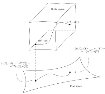
The significance of a system being flat is that all system behavior can be

expressed without integration by the flat outputs and a finite number of its

deriva-tives. That is, referring to Figure 2.3, the problem of finding curves that take the

system from x(0), u(0) to x(T), u(T) in equation (2.1) is reduced to finding any

sufficiently smooth curve that satisfies zk(0) andzk(T) up to some finite number. There is no need to solve a two-point boundary value problem if the system is

differentially flat.

Once all the boundary conditions and trajectory constraints are mapped into

the flat output space, (optimal) trajectories will be planned in the flat output space

and then lifted back to the original state and input space as shown in Figure 2.3.

The idea is that this methodology will alleviate adjoining the system dynamics in

the optimal control problem formulation. Consequently, the number of variables

in the optimal control problem will be reduced to expedite real-time computation.

It is debatable whether or not the necessary and sufficient conditions for

differ-ential flatness exist. Fliesset al. in [32] and [33] provide necessary conditions and Charletet al. [16] provide sufficient conditions for a class of systems. Chetverikov in [19] is the first to provide necessary and sufficient conditions, but the solution

appears to involve solving a set of nonlinear partial differential equations.

Al-though the work of Chetverikov is promising, one frequently has to resort to trial

and error to construct the flat outputs.

(53)

Flat space State space

x(T), u(T)

x(0), u(0)

(z(T),z(T˙ ), . . . , z(l)_(T_{)) =}

w−1_{(x(0), u(0))}

(z(0),z(0), . . . , z˙ (l)_{(0)) =}

w−1_(x(T_{), u(T}₎

Figure 2.3: A flat system has the important property that the states and the inputs

can be written in terms of the outputsz and their derivatives. Thus, the behavior of the system is determined by the flat outputs. Note that the mapw is bijective.

the initial pointx(0), u(0) to the final point x(T), u(T):

˙

x1 = x2 ˙

x2 = u1 ˙

x3 = u2cosx2 ˙

x4 = u2.

(2.73)

(54)

2.8. System Design and Differential Flatness 39

z2=x3−x4cosx2. Taking derivatives, we have,

z1 = x1 z˙1=x2 z¨1 =u1 z₁(3)= ˙u1

z2 = x3−x4cosx2 z˙2=x4sinx2u1 ¨

z2 = u2sinx2u1+x4cosx2u21+x4sinx4u˙1.

(2.74)

It can be shown that there is a local diffeomorphism between the variables

x1, . . . , x4, u2, u1,u˙1

and the variables

z1, . . . , z1(3), z2,z˙2,z¨2.

Therefore, by specifying the initial and final state, input, and auxiliary state (ξ= ˙

ui) we uniquely specify the flat outputs and their derivatives in flat output space. The problem has been resolved into one of solving an algebraic problem. Moreover,

any curve that satisfies the boundary conditions in the flat output space is a

trajectory of the original system (2.73).

Example 2.3. This example illustrates that the flat output may contain the input. This problem can be found in Martinet al. [66]:

˙

x1 = u1 ˙

x2 = u2 ˙

x3 = u1u2.

(2.75)

The flat outputs are z1 = x3 −x1u2 and z2 = x2. It can be shown that there is a local invertible map between the variables x1, x2, x3, u1, u2, u(1)₂ , u(2)₂ and the variables z1z1(1), , z

(2)

1 , z2, . . . , z2(3).

2.8

System Design and Differential Flatness

A salient feature of flight control systems is that the requirements imposed are

(55)

VTOL design.

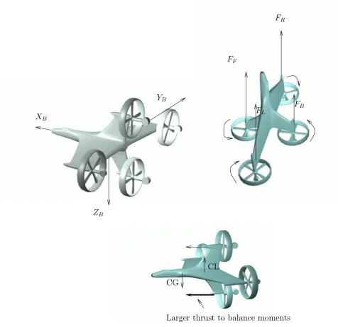
The four propeller “Aeroranger” is shown in Figure 2.4. The orientation of

FR

FF

ZB

YB

XB

CG

CL

Larger thrust to balance moments

FL

FB

Figure 2.4: The views of the “Aeroranger” show the body coordinate frame,

di-rection of rotation of the propellers, the definition of the applied forces due to the

ducted fan thrust, and a method used for stabilizing the aircraft in aerodynamic

(56)

(57)

Using Euler’s equation in body coordinates (assuming no products of inertia)

gives the rotational dynamics

Ix˙Ωx+ (Iz−Iy)ΩyΩz = MXb+MXa

IyΩy˙ + (Ix−Iz)ΩzΩx = MYb+MYa

IzΩz˙ + (Iy−Ix)ΩxΩy = MZb+MZa,

(2.79)

where Ix,Iy, and Iz are the principal moments of inertia, MXb, MYb, and MZb

are the body moments due to the differential thrust forces, MXa, MYa, and MZa

are the aerodynamic moments, and Ω1, Ω2, and Ω3 are the angular rates in body

coordinates given by

Ωx = φ˙−ψ˙sinθ

Ωy = θ˙cosφ+ ˙ψcosθsinφ

Ωz = ψ˙cosθcosφ−θ˙sinφ.

(2.80)

The body moments are

MXb = kw(FL+FR−FF −FB)

MYb = lF B(FF −FB)

MZb = lLR(FL−FR),

(2.81)

wherekw is the torque constant of the propeller, lF B is half the distance between the applied forceFF andFB, andlLR is half the distance between the applied force

FL andFR as seen in Figure 2.4.

Example 2.4. Near hover, the “Aeroranger” is differentially flat. Since the system is near hover, we will assume that the aerodynamic forces FXa, FYa, and FZa in

equation (2.78) are zero. Choose the outputs for the “Aeroranger” to be

z1 =x, z2 =y, z3 =z, z4=φ. (2.82)

Taking up to the fifth derivative of equation (2.82) and substituting equations

(58)

2.8. System Design and Differential Flatness 43 inputs, and their derivatives.

z₁(1) = x˙ z₁(2)=ζ1(cosθcosψ)

z₂(1) = y˙ z₂(2)=ζ1(cosθsinψ)

z₃(1) = z˙ z₃(2)=−ζ1sinθ−g

z₄(1) = φ˙ z₄(2) =f1(ψ, φ, θ,ψ,˙ θ,˙ φ, M˙ Xb, MYb, MZb)

z₁(3) = f2(ζ1,ζ˙1, ψ, φ, θ,ψ,˙ θ,˙ φ˙)

z₂(3) = f3(ζ1,ζ˙1, ψ, φ, θ,ψ,˙ θ,˙ φ˙)

z₃(3) = f4(ζ1,ζ˙1, ψ, φ, θ,ψ,˙ θ,˙ φ˙)

z₁(4) = f5(ζ1,ζ˙1,ζ¨1, ψ, φ, θ,ψ,˙ θ,˙ φ, M˙ Yb, MZb)

z₂(4) = f6(ζ1,ζ˙1,ζ¨1, ψ, φ, θ,ψ,˙ θ,˙ φ, M˙ Yb, MZb)

z₃(4) = f7(ζ1,ζ˙1,ζ¨1, ψ, φ, θ,ψ,˙ θ,˙ φ, M˙ Yb, MZb),

(2.83)

where

ζ1 =FL+FR+FF +FB (2.84)

is the combined force of the propellers along Xb as shown in Figure 2.4. In short,

(z1, . . . , z2(4), z2, . . . , z(4)2 , z3, . . . , z3(4), z4,z˙4,z¨4) = Ψ(ξ), (2.85)

where

ξ= (x, y, z, θ, φ, ψ,x,˙ y,˙ z,˙ θ,˙ φ,˙ ψ, M˙ Xb, MYb, MZb, ζ1,ζ˙1,ζ¨1).

The above relation is locally invertible, with the exception of a few points, since

det(∂Ψ

∂ξ) =

−ζ₁6cos 2θ−ζ₁6

2IxIyIz

in nonzero. The “Aeroranger” is differentially flat by Definition 2.3. For

(59)

ψ can be found from the following:

tanψ= z¨2 ¨

z1

. (2.86)

Second, θ can be found from the following:

tanθ= g−z¨3 ¨

z1cosψ+ ¨z2sinψ

. (2.87)

Using the information provided by two derivatives of equation (2.86), (2.87), the

flat output z4 and then substituting into equation (2.79), it is possible to recover

MXb,MYb, and,MZb. Using equation (2.84), ζ1 may be recovered from the

follow-ing:

ζ1 =m q

¨

z12+ ¨z22+ ( ¨z3−g)2. (2.88)

Finally, the applied forces may be recovered using equation (2.88) and equation

(2.81). As a result of using the two argument tangent function, we can avoid the

singularity at θ= π₂.

Remark 2.3. It is not difficult to show that the “Aeroranger” is differentially flat, when the aerodynamic forces are not negligible. However, a closed form solution

may be elusive. We will assume that actuation for this system will not only be the

thrusts due to the propellers, but also four aerodynamic surfaces, one on each wing

of the “Aeroranger”. An additional assumption is needed, that the aerodynamic

surfaces only contribute to the aerodynamic moments and not the aerodynamic

forces. We choose the flat outputs the same as those in equation (2.82). We will

assume that the aerodynamic forces are a function of V,α,β. Moreover, we will assume that the aerodynamic moments are a function of V, α, β, and δi, where

δi i= 1, . . . ,4 is the deflection angle of theith surface.

First, we will solve forψ,θandζ1. Expressions forαandβ can be determined from

tanα= w

(60)

(61)

VTOL Hover actuation Flat near Flat in forward flight?

hover?

Ducted Fan Thrust vectored ducted fan Yes Yes, with no vectoring;

unknown otherwise

Two Ducted Fans Two ducted fans Yes Yes

“Aeroranger” Four propellers Yes Yes

“Aerojeep” Four ducted fans Unknown Unknown

Table 2.1: Summary of the flatness characteristics of several simple VTOL

con-figurations. Flat in forward flight implies that the mixing of hover actuation and

aerodynamic surfaces is possible.

Two Ducted Fans

Aeroranger Aerojeep

Ducted Fan with Thrust Vectoring

g

(62)

2.9. Parameterization of the Output 47

2.9

Parameterization of the Output

In the previous section, techniques were presented to reduce or eliminate the

dy-namic constraints by selecting a special set of variables (outputs) that could

com-pletely characterize the states and inputs of the system under consideration. In

this section, we will discuss how to select the outputs from a finite dimensional

space, in order that the problem under consideration can be efficiently solved.

There are many curves that can be used to approximate the outputs (Fourier

series, polynomials, rational segments, etc.). Aside from accurately representing a

basis of the solution of the trajectory generation problem under consideration with

a reasonable number of decision variables, the main requirements of the curve are

the ability to set a level of continuity Ck_{, without adding additional constraints.} Local support is also a desirable property of the basis functions. Local support

means that the curves only influence a region of the curve local to the current

point of interest. Specifying the level of continuity is necessary, since the states

and inputs are a function of the outputs and their derivatives. Local support is favorable for numerically stable computer implementation. A high order single

polynomial would be necessary to satisfy complex constraints. Solving for the

coefficients of the polynomial would be an inefficient and ill-conditioned operation.

A solution that meets the main requirements is piecewise Bezier polynomials or

B-splines. An overview of B-splines, from which much of the following is derived,

can be found in Deboor [9].

An outputy(t) may be defined in terms an order kBezier curve by