Electronically Towed Micro Vehicles

Abstract

Sanders, Keith Aaron. Electronically Towed Micro Vehicles. (Under the direction of Dr. M.K. Ramasubramanian)

In recent years, tremendous advancements have been made in the area of intelligent vehicle systems, autonomous vehicles, and remote navigation. Applications of such advancements vary from highway transportation systems, to military convoys, to unmanned exploration of dangerous environments. The evident benefits of these intelligent vehicle systems include more efficient travel, transportation of multiple vehicles by a single driver, and remote exploration of hazardous or otherwise dangerous terrain.

The purpose of this research is to develop and implement an electronically towed micro vehicle system using a 1/10 scale R/C car as the platform. The system will use minimal external sensors and will be capable of following a lead vehicle through various maneuvers at various speeds. The scope of the project includes modifying an R/C car for autonomous control by a microprocessor, establishing a wireless link between two vehicles for direct communication, and developing a control algorithm that will enable the towed vehicle to follow a leader operated by radio control. The towed vehicle will rely on information transmitted from the leader as well as from on board sensors to determine the path of the leader and follow accordingly. Several experimental tests have been conducted to test the performance and determine the limits of the system. The results of these experiments demonstrate a working leader follower system implemented on 1/10 scale vehicles. Future development and research will be aimed at implementing this system on full scale

Electronically Towed Micro Vehicles

By:

Keith Sanders

A Thesis submitted to the Graduate Faculty of North Carolina State University

in partial fulfillment of the requirements for the degree of

Master of Science

Mechanical and Aerospace Engineering Raleigh, NC

July, 2003

APPROVED BY:

___________________________ ___________________________ Dr. Larry Silverberg Dr. Eric Klang

Dedication

Biography

Acknowledgements

I would like to thank my parents and family for giving me the opportunity to pursue a college career and supporting me throughout my endeavors.

Thanks to my graduate committee, Dr. Klang and Dr. Silverberg for allowing me to search for an interesting research project when I didn’t know what I wanted to do.

Thanks also to my graduate advisor, Dr. Ram, who gave me the mechatronics background needed to accomplish this project. Thanks for giving me the opportunity to work on this project.

I would like to thank my friends who have helped me along the way in classwork and with ideas along the way about my research. Especially Robert Hughes and Jason Stevens for their friendship and help.

I would also like to thank my community of friends and fellow Christians at Forest Hills Baptist Church, with whom I have created lasting friendships over the past 4 years. The opportunities and experiences I have gained through my involvement with Forest Hills over the past few years have encouraged and uplifted me tremendously.

Table of Contents

List of Figures... vii

List of Tables ... viii

1.

Introduction...1

1.1 Brief History of Intelligent Vehicle Systems... 1

1.2 Purpose... 2

2.

Literature Review ...3

3.

Objectives...9

4.

Platform for Implementation...10

4.1 Vehicles ... 10

4.2 Hardware ... 11

4.3 Software ... 14

5.

Leader/ Follower Control Scheme Development ...15

5.1 Open Loop ... 15

5.2 PD Velocity Control... 15

5.3 Following Distance Control... 16

5.4 Relative Position Control ... 16

6.

Final Design Structure...18

6.1 Throttle and Servo Control... 18

6.2 Input Capture Channels... 18

6.3 Serial Communication Protocol... 19

6.4 PWM Operation... 19

6.5 Control Algorithm ... 20

7.

Testing ...23

7.1 Benchtop Testing... 23

7.2 Testing simple maneuvers ... 24

8.

Results and Discussion...27

8.1 Straight Line Following... 27

8.2 Complex Paths... 29

9.

Limitations...33

10.

Conclusions...35

11.

Suggestions for Future Work ...36

List of Figures

Figure 1: Small Robot Follower Performance [6] ... 4

Figure 2: Autonomous vs. Co-operative System Performance [11] ... 6

Figure 3: Electric Tow-bar results, Tamura and Furukawa [13] ... 8

Figure 4: RC10 Truck ... 10

Figure 5: Electronics Layout... 12

Figure 6: Follower vehicle with distance sensors installed ... 13

Figure 7: Hall effect sensor mounting ... 14

Figure 8: Steering servo operation... 18

Figure 9: Control Algorithm Flow Chart ... 22

Figure 10: Benchtop Testing of Vehicles ... 23

Figure 11: Testing Follower Algorithm... 24

Figure 12: Path Following Test Initialization ... 26

Figure 13: Distribution of Error for 50 runs ... 27

Figure 14: Longitudinal Distance Graph ... 28

Figure 15: Complex Path Following Test... 29

Figure 16: Path following experimental results ... 30

Figure 17: Graphical representation of path following results ... 31

Figure 18: Lateral Error vs. Distance Traveled ... 32

Figure 19: CCD diagram (taken from www.sensorsmag.com) ... 36

Figure 20: Distance and Orientation Diagram ... 37

Figure 21: HC08 Development Board Layout... 64

Figure 22: Pinout connections for Leader Vehicle ... 64

Figure 23: Pinout diagram for Follower vehicle... 65

Figure 24: Hall effect sensor wiring diagram ... 65

Figure 25: Bluetooth implementation schematic ... 66

Figure 26: GP2D12 Analog Value vs. Distance Plot... 68

Figure 27: Longitudinal Distance Graph (Run 2) ... 68

List of Tables

1.

Introduction

Automotive vehicles are becoming more and more intelligent each year. From cruise control to anti-lock brakes to roll control systems for SUVs, emerging technologies are being

developed that increase the safety and driveability of automobiles.

1.1 Brief History of Intelligent Vehicle Systems

The first intelligent vehicle systems were cruise control devices. An engineer named Ralph Teetor, blind from the age five, invented and patented a speed cruise control device in 1945. By 1960, all major car manufacturers offered cruise control, and today, all cars are available with cruise control.

Another major advancement in vehicles came with the addition of electronic anti-lock brake systems. Anti-lock brakes were offered in the 70’s, and more recent technological

advancements have greatly improved these systems.

The most recent advancements include smart airbag systems that make decisions based on impact severity, mass of occupant, and other factors. Anti-rollover systems have also been implemented to make SUV’s safer.

1.2 Purpose

2.

Literature Review

Autonomous and automated vehicle systems have received considerable amounts of research attention in recent years. The advantages of intelligent vehicle systems in today’s

transportation include more efficient and safer travel, as well as increased comfort for passengers. More specifically, leader-follower systems, or automatically towed vehicles have become the subject of increased amounts of research. Several of these papers will be discussed here to establish the current technology and capabilities of these systems.

Figure 1: Small Robot Follower Performance [6]

Rajamani [10] in conjunction with the PATH Program in California demonstrated an automated highway platoon system in 1997. The demonstration consisted of a platoon of eight vehicles traveling at 60 mph with a spacing of 6.5 meters. The system uses inter-vehicle communication, radar sensors, and magnetic sensors for measuring lateral position relative to the lane center to maintain the correct following behind the leader. This system was shown to work well for vehicles traveling at highway speeds. The drawback to this system is that it requires magnetic markers to be buried along the centerline of each lane with 4 ft spacing.

vehicle and the following vehicle. It does not rely on any other information and is designed to be robust for use in vehicles with different dynamic characteristics. Simulations verify the performance of this system under different driving scenarios.

Rajamani and Shladover[11] studied the performance of autonomous and co-operative vehicle follower control systems. This study documented the advantages obtained through different levels of co-operation between the vehicles. Typical autonomous follower systems can achieve an vehicle spacing of about 30 meters at highway speeds. Large inter-vehicle spacing promotes unsafe cut-ins and inefficient highway travel. The co-operative vehicle system replaced the radar range rate data with the difference in wheel speeds of the two vehicles. Using the co-operative vehicle system, inter-vehicle spacing of 6.5 meters was maintained in an 8 car platoon. This greatly enhances traffic flow efficiency without

Figure 2: Autonomous vs. Co-operative System Performance [11]

identifies the lead vehicle as well as lane markings to maintain its heading along the path. Simulations have been conducted to verify the performance of this system. This research shows the possibilities of a leader follower system when unlimited resources and information is available to the follower vehicle.

Tamura and Furukawa[13] developed an electric tow-bar system for vehicles traveling in platoons, which was presented at the IEEE Intelligent Vehicles Symposium 2000. A system free from external infrastructure has been developed using laser radar sensing systems and inter-vehicle communication and navigation system. A maximum of five vehicles track a lead vehicle at a distance of two meters at speeds up to 100km/hr. The following system calculates the position and orientation of each vehicle by using a navigation system installed on both the lead vehicle and follower vehicles. This information is relayed to the follower vehicles using the inter-vehicle communication. The follower vehicle uses this information to put together the trace path of the leader vehicle. In addition to the communicated

3.

Objectives

The objectives of this research will be to build to design and build an electronically towed micro vehicle system. The system will meet the following design criteria:

• Co-operative leader follower system • Mobile infrastructure

• Minimal use of sensors

4.

Platform for Implementation

This section discusses the platform that was selected for the research and details the components of the vehicles selected.

4.1 Vehicles

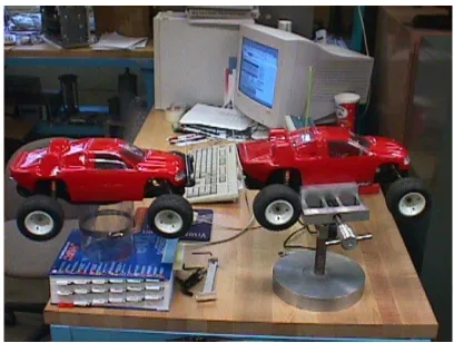
The vehicles are 1/10 scale radio controlled cars. Specifically, they are RC10 off-road trucks manufactured by Team Associated. These vehicles provide a robust platform capable of relatively high speeds (up to 25 mph), good maneuverability, and durability. The picture below shows the RC10 truck that is used as the leader.

4.2 Hardware

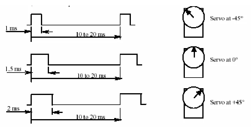
The vehicles are equipped with Futaba S3003 servos to control position of the steering, while an LRP electronic speed control drives the permanent magnet DC motor. The steering position is proportional to a 1 to 2 ms pulse input to the servo. A 1.5 ms pulse positions the steering straight, while 1 ms is hard left, and 2 ms is hard right. The input to the speed control is similar. A 1.5 ms pulse is neutral, 1ms is full brake, and 2 ms is full speed

forward. The inputs to the servo and speed control on the leader vehicle come from the AM receiver, which is controlled by a radio control transmitter. The follower vehicle is

controlled directly by the microprocessor.

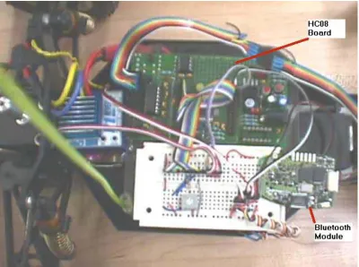
Each car is fitted with a Motorola HC08 microprocessor. An evaluation board by Elektronikladen houses the Motorola MC68HC908GP32 processor as well as a crystal, memory, I/O pins, and an RS232 interface for serial communication. The HC08 processor is used to gather information from onboard sensors, communicate between the two vehicles, and implement control techniques to maneuver the follower vehicle.

Figure 5 shows the layout of the electronics on the RC10 vehicle. The HC08 processor, BL-730 bluetooth module, breadboard, and electronic speed control are all shown in this picture. These components are mounted on an elevated piece of plexiglass. The steering servo and battery pack are mounted beneath the plexiglass.

The processor is supplemented with GP2D12 infrared distance sensors. These sensors provide analog distance values that are used to maintain alignment and safe distances

between the lead vehicle and the follower. The follower uses three distance sensors mounted on the front of the vehicle to determine following distance and lateral alignment. The

mounting of these sensors is shown below.

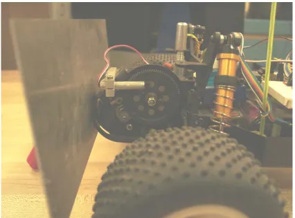
Hall effect sensors, along with 8 magnets mounted in the pinion gear of the transmission provide position and velocity data. The picture below illustrates the mounting of the hall effect sensor.

Figure 7: Hall effect sensor mounting

4.3 Software

5.

Leader/ Follower Control Scheme Development

The control algorithms for the vehicles have been developed mainly based on experimental trial and error complimented by a background in basic control theory. This section will outline the development of the current algorithm as it was developed.

5.1 Open Loop

The first control scheme was an open loop controller with no feedback. For this trial, the follower was made to mimic the leader exactly with regard to steering and throttle position with a fixed time delay between the two vehicles. Perhaps this would work well in a perfect system. That is, if the two cars were identical in terms of vehicle dynamics, traction, steering and throttle rates, battery voltage, etc., the follower could mimic the actions of the leader and be made to follow the same path. Although the vehicles used for this research are identical cars with identical motors, the differences in the characteristics of each vehicle are enough that attempting to use an open loop controller is futile. Feedback through sensors must be used to detect these differences and adjust accordingly.

5.2 PD Velocity Control

the response of the controller. The P gain is the equivalent of a spring in a mechanical system. The larger the error, the larger the applied ‘force’ to the system. The D term adds control based on the derivative of the error term. This serves as an artificial damper for the system. The proportional and derivative terms are combined into the total control effort and are added to the throttle output of the motor.

5.3 Following Distance Control

Due to the characteristics of the motors and vehicles, it was soon apparent that velocity control would be difficult. By adjusting the gains of the controller, the response could be optimized, but this only seemed to work well at a specific speed. Since the vehicle must obviously operate at varying speeds, this option was soon abandoned. The next idea was to control the following distance of the follower vehicle. The distance was measured using the Sharp infrared sensors. An optimal following distance of 12 inches was prescribed, and a PD controller was implemented to maintain this distance. The sensor provided an analog signal to the processor based on the distance between the two vehicles. The problems with this type of algorithm were apparent early. One problem was that the analog signal does not follow a linear relationship with distance. This makes it difficult to determine the actual distance based on the analog signal. Another problem was that the sensor is not always facing the lead car. For example, when the lead car makes a turn, the follower will not be directly behind the leader and will therefore give a faulty distance reading. The algorithm was modified to function only when the two cars were both traveling straight, but this left no control during turns. This type of control was determined not robust or accurate enough to work for this system.

5.4 Relative Position Control

6.

Final Design Structure

6.1 Throttle and Servo Control

Control of the throttle and steering is accomplished by using the PWM capabilities of the HC08 processor. The steering angle of the servo is proportional to a pulse sent to the servo. The pulses are sent at a rate of 50 Hz. A pulse of 1ms rotates the servo to its extreme left position, while a 2ms pulse rotates the servo to its extreme right position. 1.5ms is the neutral position. The diagram below illustrates the servo operation. On the left is the signal from the microprocessor, and the right shows the rotation of the servo. The throttle control operates the same way, but a 1ms pulse is full brake and a 2ms pulse is full forward.

Figure 8: Steering servo operation

6.2 Input Capture Channels

control, and consequently the steering angle and throttle position. Steering angle and throttle position were relayed to the follower vehicle and stored.

6.3 Serial Communication Protocol

Once the vehicles were capable of operation by the processor, communication between the two vehicles was necessary. The Serial Communications Interface (SCI) Module on the HC08 allows for this communication. The SCI module is capable of transmitting and

receiving data at programmable baud rates. For this project, the lead vehicle transmitted data to the follower vehicle. This data included speed, position, steering angle, and a checksum value. The checksum routine ensured that the data transmitted was valid and not corrupt. The follower vehicle used the SCI receiver to receive data and a subroutine to sort the data and store it in arrays. This allowed the follower to mimic the actions of the leader with a time delay. The SCI is configured to send data at a rate of 16 Hz, but is capable of much higher rates.

6.4 PWM Operation

6.5 Control Algorithm

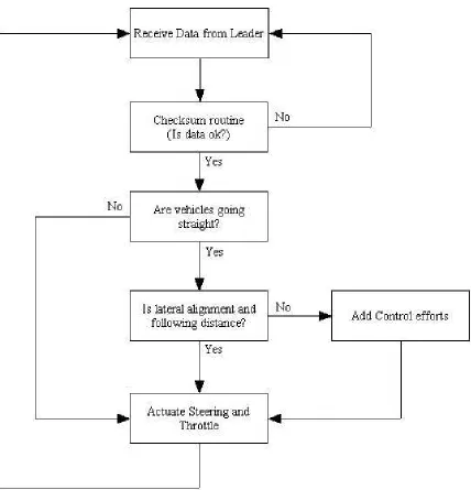
The current control algorithm is a result of experimental results based on the techniques previously outlined. The control scheme that worked the best seemed to be the relative position control. The number of revolutions of the transmission gear was directly related to distance traveled, and relatively precise. Implementing a simple P controller seemed to be sufficient to control the following distance of the follower vehicle. Additionally, the position of the vehicle was coupled with the steering angle. In this way, the follower vehicle was made to turn at the same location that the leader turned. Since the steering servos and linkages do not behave exactly the same, it was apparent that some type of control would be needed for the steering as well. This became more difficult than the throttle control. Only slight differences in steering angles would send the car in significantly different directions. A pair of GP2D12 sensors was mounted on the front of the follower car. The sensors were positioned on each side of the vehicle facing forward, so that they both lined up with the rear of the lead vehicle. If the follower veered to the left, the left sensor would lose sight of the leader and the follower would correct by steering back to the right. This control fails during turns since the follower car is not directly behind the leader through turns. To avoid this problem, steering control was only implemented when the two vehicles were going straight and were directly behind each other. Thus far, this control scheme works the best. However, this controller depends on the cars going straight to control the steering. If the lead car makes too many turns, the follower will eventually get off track and lose sight of the lead vehicle. The flow-chart in Figure 9 shows an outline of the actions taken by the follower vehicle. The flow-chart significantly simplifies the algorithm so it is easier to understand. The following sections define the operation of the leader and follower vehicles.

6.5.1 Leader

information to the follower. The radio transmitter communicates with the receiver on board, which then sends a signal to the servo and speed control. These two signals are also sent to the input compare pins on the HC08. The HC08 measures the pulse width of each signal, and relays the data to the follower. The HC08 also counts the number of magnets that pass by the hall effect sensor. This, in conjunction with a Time-based interrupt that occurs at a rate of 16 Hz, is used to measure position and velocity which is also relayed to the follower. All this information is sent through the SCI using the bluetooth wireless serial port converter. The bluetooth module communicates at 115,200 baud, but is capable of even faster data transfer rates.

6.5.2 Follower

The follower has a tougher job than the leader. It must collect information from the leader and onboard sensors, store this information for later use, and control the speed and direction of the vehicle based on the gathered information. The information received from the leader includes position, throttle, steering angle, and rpm. This data is the baseline for the actions of the follower. Ideally, the follower mimics the leader with a built in time delay. If the two vehicles were identical, then theoretically, the follower would follow the exact path as the leader. Slight differences in the behavior of the two vehicles make this impossible. This is where the sensors on the follower vehicle come in. The hall effect sensor is used to

7.

Testing

Extensive testing was done throughout the development of the algorithms and control schemes. The system was broken up into many smaller subsystems and each of the

subsystems tested and fine-tuned individually. Once each of the subsystems were functional, they were combined to comprise the current system. This section outlines some of the testing that was done during the research.

7.1 Benchtop Testing

Throughout the various stages of development, I tested the code continuously with the cars suspended on stands. This allowed me to test each part of the code and verify that they were working before actually putting the cars on the ground. Once the cars were operating

7.2 Testing simple maneuvers

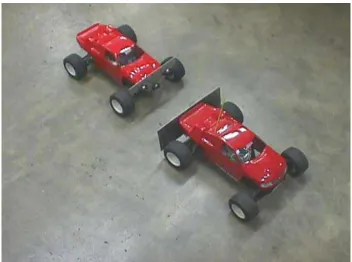
Once the code was working, the cars were tested under different maneuvers. This will help define the limits of the control scheme and provide insight about what should be done to improve the performance. Figure 11 below shows the two vehicles ready to go.

Figure 11: Testing Follower Algorithm

7.2.1 Straight Line Following

The first test was conducted by driving the lead vehicle in a straight line. The main objective of this phase of testing was to adjust the gains on the throttle control so the follower would be able to maintain a relatively constant following distance. It was also used to adjust the

neutral position of the steering servo. Once these variables were adjusted, experimental data was collected to determine the precision of the follower. The lateral error as well as

required another method of data acquisition to be developed. Since the longitudinal error must be measured in real time as the experiment was being conducted, it required capturing data from the microprocessor as the experiment was conducted. The problem with this is that the SCI interface is already taken by the Bluetooth module. To overcome this, the Serial Peripheral Interface (SPI) was used to send information to an additional HC08 processor. This processor then relayed the information to a laptop PC using the SCI. The results of these experiments are tabulated in the results section

7.2.2 Complex Paths

8.

Results and Discussion

This section lists and explains the results of the experimental tests conducted to evaluate the performance of the electronically towed micro vehicle system.

8.1 Straight Line Following

Figure 13 below shows the distribution of the lateral error of the follower car for straight line driving at two different speeds. As can be seen from the graph, the follower performs well at a speed of 2 mph. The error is less than 5 inches for all runs, and is zero for 22 out of the 50 runs. The test was also done at 4 mph, or about twice the speed of the first test. As expected, the performance declined significantly. The majority of the runs had less than 5 inches of lateral error, but some of the errors are significantly higher.

Distribution of Error

10 15 20 25

The longitudinal error was also recorded for the straight line tests. Figure 14 shows the longitudinal following distance as a function of distance traveled. The optimal distance is 18 inches. The data from the figure was captured using the difference in the number of counts of the hall effect sensors, which was converted to a distance. This particular run was conducted at about 4 mph, which is a moderate speed for these vehicles. Plots for several other runs are included in Appendix D.

Figure 14: Longitudinal Distance Graph

The graphs above show the performance of the following distance controller. Over the 100 ft test run, the following distance varies about ±2 inches throughout the test with one small spike in the data. These results are very good considering the size of the vehicles and the speed at which the test was conducted. The controller is very responsive and maintains

Follow ing Distance vs. Distance travelled

12 14 16 18 20 22 24

0 10 20 30 40 50 60 70 80 90 100

Distance travelled (ft)

F o llo w in g D ist an ce ( in )

Velocity vs. Distance travelled

0 1 2 3 4 5 6

0 10 20 30 40 50 60 70 80 90 100

Distance travelled (ft)

factor in this test. The current sensor uses only eight magnets per gear revolution which translates to about 1.5 inches of travel per magnet. Hence, using a better encoder would provide much more accurate feedback and improve the performance of the controller.

8.2 Complex Paths

Figure 16 shows the results of one of these tests. From the picture you can see the paths taken by the leader and follower. The course consisted of one 90 degree turn, three 180 degree turns and several straight segments. The cars traveled at low speed, approximately 2 mph throughout the course. The cars performed well during the test, with one exception. The follower oversteered through one 180 degree turn, but this may have been caused by the markers dragging on the edge of the paper. Aside from that the performance was acceptable.

Figure 17 shows a graphical representation of the test results. Once the vehicles completed the paths, points were added at approximately one-foot intervals. The coordinates of each of these points were recorded and plotted in Excel. This allowed for a quantitative measure of performance based on the error between the two paths. You can see from the graph that the follower followed the general path of the vehicle

Leader and Follower Paths

0 20 40 60 80 100 120 140 160

0 20 40 60 80 100 120 140 160

Horizontal Distance (in)

Vertical Distance (in)

Leader

Follower

Figure 17: Graphical representation of path following results Start

The distance between the points of the leader and follower defines the error of the follower. Figure 18 plots this error as a function of distance traveled. The error has been normalized to the width of the vehicle to better illustrate the error relative to the size of the vehicle. The error remains less than 0.6 times the car’s width, which is satisfactory. One important note is that the vehicles were repositioned about halfway through the test. The markers caught the edge of the paper and impaired the vehicles’ movement.

Lateral Error vs. Distance traveled

-1.0 -0.5 0.0 0.5 1.0

0 10 20 30 40 50 60

Distance traveled (ft)

Lateral Error (Normalized)

9.

Limitations

The current leader follower algorithm has limitations. First, the relative orientation of the follower with respect to the leader could not be accurately measured. The distance sensors on the front of the follower detect the following distance, but not orientation. The resolution of the sensors also limits the ability to accurately measure distance. The signal from the infrared sensors fluctuates depending on several factors including reflectivity of the surface, temperature, and angle of surface with respect to the sensor. These factors along with the fact that the output voltage does not vary linearly with distance make it difficult to obtain accurate distance measurements from the GP2D12 sensors.

A second limitation to the vehicles is related to the steering mechanisms. There are slight differences in the servos, steering linkages, and front tires of the two vehicles. Since the feedback control is internal to the servo, we have no feedback on the actual steering angle of the front tires. These differences cause the vehicles to become misaligned over a period of time. Even if the error is very small, over time the error increases and with no feedback causes the follower to go astray.

Maneuvering through a tight course with many turns will result in the follower straying from the path over time. The vehicles will perform better when following a path with only slight turns and sufficient time on straight paths, similar to interstate driving.

A final limitation to the leader follower system is the presence of external obstacles. The follower relies on information from the front distance sensors to maintain its course behind the lead vehicle. The sensors cannot distinguish between different objects; they are only able to determine the distance from the object. This would make driving around obstacles

10.

Conclusions

This paper outlines the development of an electronically towed vehicle system implemented on 1/10 scale R/C vehicles. After selecting the RC10 as a platform, the vehicles were

11.

Suggestions for Future Work

The current performance of the leader follower vehicle is less than perfect. This section will outline what is needed to improve the performance of the vehicles.

11.1Distance and Orientation Sensors

the two vehicles, α, is determined from the following relationships. First, the length

(

)

1

2 d w

d

h= − + , then the angle α can be obtained using

h w

1 sinα ₌

.

11.2 Vision based follower

As discussed in the background section, several other similar research projects utilize vision based sensing to determine relative position of the lead vehicle with respect to the follower. There are several advantages that this type of system can offer to the project. Whereas the current sensors only sense the position of two points on the rear of the lead vehicle, a video camera could ‘see’ the leader and determine the position based on the coordinates of certain points on the leader. Also, a vision based system could distinguish between the lead vehicle and other vehicles or objects that may be in the path of the follower. The current system simply assumes that the leader is in front of the follower and cannot distinguish between the leader and other objects. Cheok et. al. outline a perception algorithm that determines position of the leader based on the width / height ratio of a rectangle positioned on the rear of the lead vehicle.

11.3 Adapting to Full Scale Vehicle

12.

References

[1] Brainboxes. www.brainboxes.com BL-703 Product Manual

http://www.brainboxes.com/products/bluetooth/product.asp?id=BL-730 2003

[2] Cheok, K.C., Smid, G.E., and Kobayashi, K, “A Fuzzy Logic Intelligent Control System Architecture for an Autonomous Leader-Following Vehicle”, Dept of Electrical and Systems Engineering, Oakland University, Rochester, MI.

[3] Cheok, K.C., Smid, G.E., Kobayahshi, Kazuyuki, Overholt, James, and Lescoe, Paul “A Fuzzy Logic Intelligent Control System Paradigm for an In-Line-of-Sight

Leader-Following HMMWV”, Journal of Robotic Systems, pps. 408-420, 1997

[4] Dumberger, Martin, “Taking the Pain out of Laser Triangulation”, Sensor Teechnology and Design. http://www.sensorsmag.com/articles/0702/laser/main.shtml

[5] Hessburg, Thomas, and Tomizuka, Masayoshi. “An Adaptation Method for Fuzzy Logic Controllers in Lateral Vehicle Guidance”, PATH Research Report, 1995

[6] Hogg, Robert W. et. al. “Sensors and Algorithms for Small Robot Leader/Follower Behavior”, Jet Propulsion Laboratory – California Institute of Technology

[7] Ioannou, P, and Xu, Z. “Throttle and Brake Control Systems for Automatic Vehicle Following”, Southern California Center for Advanced Transportation Technologies, 1994

[8] Lee, G.D., and Kim, S.W., “A longitudinal control system for a platoon of vehicles using a fuzzy-sliding mode algorithm”, Electrical and Computer Engineering Division,

POSTECH University, South Korea. Mechatronics 12 pps. 97-118, 2002

[9] Motorola. www.motorola.com 68HC908GP32 Brochure.

http://e-www.motorola.com/files/microcontrollers/doc/brochure/BR1793.pdf 1999

1823-[14] Tan, Yaolong and Kanellakopoulos, Ioannis. Longitudinal Control of Commercial Heavy Vehicles: Experimental Implementation.

Appendix A: Technical Specifications

Overview from www.motorola.com

The Motorola 68HC908GP32 provides designers with a highly integrated 8-bit FLASH microcontroller (MCU) solution. The 68HC908GP32 builds on the success of the 68HC05 family by offering a code compatible migration path to higher performance FLASH MCUs.

Features

• 32,256 bytes of in-system programmable FLASH memory

• FLASHwire technology – a single wire interface for in-circuit programming which does not require high voltage for entry

• 10,000 program/erase cycles

• FLASH programming as fast as 2 msec for a 64 byte block • FLASH memory security features

• 512 bytes of user RAM

• High-performance 68HC08 CPU core – Code compatible with 68HC05

– 8.0 MHz internal operating frequency at 5.0 V • Peripheral modules

– Computer Operating Properly (COP) watchdog – SCI asynchronous serial communications port - Full duplex operation

- 32 programmable baud rates - Interrupt driven operation - 8-bit or 9-bit character length

– SPI synchronous serial communications port - Full duplex operation with master and slave modes - Up to 4 MHz master, and 8 MHz slave mode frequencies – 8-channel 8-bit analog-to-digital-converter

– External interrupt mask bit and acknowledge bit • Illegal address reset

• Illegal opcode reset

• Low Voltage Inhibit with selectable trip points • Clock options

– 32 KHz crystal compatible oscillator and on-chip PLL – External clock

• Bi-directional RESET pin

• Power-saving Stop and Wait modes

• 40-pin DIP, 42-pin SDIP, and 44-pin QFP packages • Pin compatible with the 68HC908GP20

• VDD/VSS pins adjacent for easy bypass capacitor connection

• Hyper-text linked on-line databook: – MC68HC908GP32/H

• Cost effective, full-featured development tools that support programming, in-circuit debug, simulation,

Comprehensive Development Support

A.2 BL-730 RS232 Bluetooth Module

Introduction

BL-730 is an RS232 (EIA232C) Bluetooth converter. It plugs onto any standard 9 pin RS232C serial port and allows the data to be sent across a Bluetooth connection to another Bluetooth enabled device that supports the serial port profile. BL-730 does not require any of the devices to which it connects to be aware that it is connected via Bluetooth.

BL-730 can also be supplied as a module (PCB only) for embedding into customer products. This document serves to deliver important information required by such system developers. The information contained within this document is believed to be accurate for the revision of the product supplied at the time the document was written. Brain Boxes Limited reserve the right to alter these specifications at any time, and particularly when creating any new revisions of the products.

Connector Type

JST 10 WAY HOUSING – Manufacturer’s Part No. SHR-10VS-B.

Connector Pin Outs

(Note. To locate Pin 1, Use the overview diagram on the previous page). PIN 1 – TXD (Transmitted Data)

PIN 2 – RXD (Received Data) PIN 3 – VSS (Ground)

PIN 4 – CTS (Clear to Send) PIN 5 – RTS (Request to Send)

PIN 6 – VEXT (Power Supply – 5V @ 300mA) PIN 7 – PIN 10 – Used Internally – NOT FOR USE.

Power requirements

The BL-730 Module requires a power input of 300 mA @ 5V.

Mounting Points

There is currently only 1 location for mounting the BL-730 PCB. These are identified below.

Bluetooth Qualification Implications

product. Brain Boxes may be able to assist you with this process – Please contact your sales representative for more details.

Version History

Versio n

Date Author Checked

By

Comments

Appendix B: C Code

B.1.1 inputs.c

/* file: inputs.c *

* This file contains the code used to retrieve digital and analog values from

* the input ports on the HC08 * -Written by Keith Sanders 8/5/03 */

int digA(int p) {

/* This routine measures digital value of PORTA pins 0-7

*/

unsigned char i;

int status;

//DDRA = 0;

i = PTA;

status = (((1 << p) & i) == 0);

return status; }

int digC(int p) {

/* This routine measures digital value of PORTC pins 0-6

*/

unsigned char i;

int status;

//DDRC = 0;

i = PTC;

status = (((1 << p) & i) == 0);

return status; }

*/

int num;

DDRB = 0; //Set Port B Data Direction register for input

if(pin == 0) {

ADSCR = 0;

while ((ADSCR & 128) != 128) //Do nothing until conversion is complete

{

}

num = ADR;

}

else if(pin == 1) {

ADSCR = 1;

while ((ADSCR & 128) != 128)

{

}

num = ADR; }

else if(pin == 2) {

ADSCR = 2;

while ((ADSCR & 128) != 128)

{

}

num = ADR; }

else if(pin == 3) {

ADSCR = 2 + 1;

while ((ADSCR & 128) != 128)

{

}

{

}

num = ADR; }

else if(pin == 6) {

ADSCR = 4 + 2;

while ((ADSCR & 128) != 128)

{

}

num = ADR; }

else if(pin == 7) {

ADSCR = 4 + 2 + 1;

while ((ADSCR & 128) != 128)

{

}

num = ADR; }

return(num); }

B.1.2 delay.c

/* file: delay.c *

* This file is used for a delay function on the HCO8 processor *

*/

void delay1ms(void) {

// 122 * [10] = 1220 cycles

// at 1.2288MHz Bus Clock -> 0.993ms asm("\

lda #122 ; \n\

loopa: nop ; [1] \n\

nsa ; [3] \n\ nsa ; [3] \n\ dbnza loopa ; [3] \ ");

}

void delay(unsigned int ms) {

while(ms--) {

delay1ms(); }

B.2 Leader Code

B.2.1 final_lead.c

/* file: final_lead.c *

* This file contains the program for the leader vehicle in the Electronically

* Towed Micro Vehicles project. The program gathers information from the AM

* radio receiver for throttle and steering position as well as from the hall

* effect sensor for speed and position. It sends this information to the

* follower vehicle using the SCI via the Bluetooth module. *

* -Written by Keith Sanders 8/5/03 */ #include <iogp32.h> #include <stdio.h> #include "vector_leader.c" #include "inputs.c" #include "delay.c" void TBM_ISR(void); void T1CH0_ISR(void); void T2CH0_ISR(void); void T2CH1_ISR(void); void initialize(void); void scisend(int num);

int rpm, rev, tot_rev, speed, revof;

int throttle, scival, steer_rate, checksum;

int throttleh, throttlel, steer_rateh, steer_ratel; int time0h, time0l, time1h, time1l, time0, time1; int oldtime0, oldtime1, pulse0, pulse1;

int spidata, x;

//throttlel = throttle - throttleh * 256;

if (pulse0 < 2000)

{

steer_rate = (pulse0 - 920) / 4;

}

//steer_rateh = steer_rate / 256;

//steer_ratel = steer_rate - steer_rateh * 256;

for (i = 0, checksum = 0; i <= 7; i++) //This loop

calculates the checksum value

{

bit1 = (((1<<i) & throttle) == 0); bit2 = (((1<<i) & tot_rev) == 0);

bit3 = (((1<<i) & revof) == 0); bit4 = (((1<<i) & steer_rate) == 0);

checksum = checksum + bit1 + bit2 + bit3 + bit4;

}

//printf("rpm = %d tot_rev = %d rev of = %d spidata = %d\r\n",rpm, tot_rev,revof,spidata);

//printf("totrev = %d",tot_rev);

//printf("throt = %d steer = %d ",throttle, steer_rate);

//printf("p1 = %d \tp0 = %d \r\n",pulse1,pulse0); //printf("time 1 = %d\r\n",time1);

scisend(255); scisend(200); scisend(throttle); scisend(tot_rev); scisend(revof); scisend(steer_rate); scisend(checksum); } }

void initialize(void) {

asm("sei"); //Disable interrupts globally

Setup_interrupt_vectors(); // Call function to setup int vector addresses

PTDPUE = 128 + 64 + 32 + 16; //Enable internal pullup for Input compare channels

T2SC = 32 + 16 + 2 + 1; // Scale TIM clock to internal clock / 8

T2MODH = 72; // Set TIM overflow value

T2MODL = 0;

T1SC0 = 64 + 4; //Enable TIM1 CH0 Interrupt, Capture on

rising edge

T2SC0 = 64 + 8 + 4; //Enable TIM2 CH0 Interrupt, Capture

T2SC ^= 32; //Clear STOP bit, make TIM counter active

T1SC ^= 32; //Clear STOP bit, make TIM counter

active

TBCR = 32 + 4 + 2; //Enable Timebase and Timebase Interrupt, Rate = 16Hz

SCDR = 0; //Write zero to SCI data register

SCC1 = 64; //Enable the SCI

SCC2 = 8; //Enable the transmitter, Write 1 to

TE

SPCR = 128 + 8 + 2; //Enable SPI, master mode, enable

receiver interrupt

asm("cli"); //Enable interrupts globally

DDRC = 4; //Set PTC2 to output

oldtime0 = 0; oldtime1 = 0; tot_rev = 21;

}

void scisend(int num){

int scistatus;

while((SCS1 & 64) == 0)

{

}

scistatus = SCS1; //read SCI status register 1

SCDR = num; //Write output to SCDR

}

#pragma interrupt_handler TBM_ISR void TBM_ISR(void){

TBCR |= 8; //Clear TBIF rpm = rev;

rev = 0;

}

#pragma interrupt_handler T2CH0_ISR void T2CH0_ISR(void){

T2SC0 ^= 128; //Clear T2CH0 flag time0h = T2CNTH;

time0l = T2CNTL;

time0 = time0h*256 + time0l; if (time0 <= oldtime0)

{

pulse0 = 18432 + time0 - oldtime0; }

else {

pulse0 = time0 - oldtime0; }

oldtime0 = time0;

}

#pragma interrupt_handler T2CH1_ISR void T2CH1_ISR(void){

T2SC1 ^= 128; //Clear T2CH1 flag time1h = T2CNTH;

time1l = T2CNTL;

time1 = time1h*256 +time1l; if (time1 <= oldtime1) {

pulse1 = 18432 + time1 - oldtime1; }

else {

pulse1 = time1 - oldtime1; }

oldtime1 = time1;

}

B.2.2 vector_leader.c

/* pseudo vector setup for Welcome Kit HC08

* example file on how to set up interrupt handlers for the welcome kit HC08.

* *

* How to modify this file:

* 1) reset vector is setup in crt08.s to point to the __start label. No * changes is needed.

* 2) For different HC08 device, change the #pragma abs_address below * to start at the address of the first vector for that device. * Change the entries to correspond with the device.

* 5) Don't forget that in the file that defines the interrupt, you must * use the #pragma interrupt_handler function

* before the definition of the function *

*/

/*

* This file has been modified to use the interrupts for the Timebase module,

* the Timer Interface Module for the three input capture channles used. *

* -Modified by Keith Sanders 8/5/03 */

extern void TBM_ISR(void); extern void T1CH0_ISR(void); extern void T2CH0_ISR(void); extern void T2CH1_ISR(void);

/* Dummy Interrupt Handler

* Place a Breakpoint here in case you are looking for spurious Interrupts */

#pragma interrupt_handler isrDummy void isrDummy(void)

{ }

void Setup_interrupt_vectors(void) {

//asm("sei"); /*Disable interrupts globally */

*((unsigned char *)0x020D)=0xCC; /*jump instruction*/ *((void(**)())0x020E)=TBM_ISR; /*address of Timebase ISR*/

*((unsigned char *)0x0210)=0xCC; /*jump instruction*/ *((void(**)())0x0211)=isrDummy; /*address of ADC ISR*/

*((unsigned char *)0x0213)=0xCC; /*jump instruction*/ *((void(**)())0x0214)=isrDummy; /*address of KBI ISR*/

*((unsigned char *)0x0225)=0xCC; /*jump instruction*/ *((void(**)())0x0226)=isrDummy; /*address of TIM2 OVR*/

*((unsigned char *)0x0228)=0xCC; /*jump instruction*/

*((void(**)())0x0229)=T2CH1_ISR; /*address of TIM2 channel 1 ISR*/

*((unsigned char *)0x022B)=0xCC; /*jump instruction*/

*((void(**)())0x022C)=T2CH0_ISR; /*address of TIM2 channel 0 ISR*/

*((unsigned char *)0x022E)=0xCC; /*jump instruction*/ *((void(**)())0x022F)=isrDummy; /*address of TIM1 OVR*/

*((unsigned char *)0x0231)=0xCC; /*jump instruction*/

*((void(**)())0x0232)=isrDummy; /*address of TIM1 channel 1 ISR*/

*((unsigned char *)0x0234)=0xCC; /*jump instruction*/

*((void(**)())0x0235)=T1CH0_ISR; /*address of TIM1 channel 0 ISR*/

*((unsigned char *)0x0237)=0xCC; /*jump instruction*/ *((void(**)())0x0238)=isrDummy; /*address of CGM ISR*/

*((unsigned char *)0x023A)=0xCC; /*jump instruction*/ *((void(**)())0x023B)=isrDummy; /*address of IRQ ISR*/

*((unsigned char *)0x023D)=0xCC; /*jump instruction*/ *((void(**)())0x023E)=isrDummy; /*address of SWI ISR*/

//asm("cli"); /* Enable Interrupts Globally */ }

B.3 Follower Code

B.3.1 final_fol.c

/* file: final_fol.c *

* This file contains the program for the follower vehicle in the Electronically

* Towed Micro Vehicles project. The program receives information from the lead

* vehicle and manipulates the throttle and steering to follow the lead vehicle.

* It uses the SCI to communicate with the lead vehicle via a Bluetooth wireless

* adapter. The throttle and steering are control by PWM signals from the Timer

* Interface Module.

#include <iogp32.h> #include <stdio.h> #include "vector_follower.c" #include "inputs.c" #include "pwm_final.c" #include "delay.c"

int tweak_steer, frontdist, left, right, steer_max, steer_min, align_steer;

int x, timedelay, realdist, go, turn;

int throttle, step, stepdelay, rpm_set, throt_set, throt_adjust; int rpm, rpm_rec, lead_rpm, rev, tot_rev, lead_rev, rev_rec, old_lead_rev; //rpm, revs

int revof, absrev, revof_rec, speed, steer_rate;

int scival;

int steer_rec, throt_rec, checksum_rec;

int lead_rpm, lead_speed, lead_steer, lead_throt, lead_absrev, lead_revof;

char throtarray[11]; //array containing throttle

data from lead car

char steerarray[201]; //array containing steering

data from lead car

void TBM_ISR(void); void T1CH1_ISR(void); void SCIRF_ISR(void); void initialize(void); void main() {

int i, j, k, checksum, bit1, bit2, bit3, bit4, reset;

initialize();

while(1) {

PTC ^= 4;

frontdist = 255 - analog(0);

left = analog(1); right = analog(3); reset = digC(0);

absrev = revof * 200 + tot_rev;

for (j = 0; j <= 201; j++) //This loop sets initial steering

{

steerarray[j] = 120;

}

for (j = 0; j <= 10; j++) //This loop sets initial

throttle

{

throtarray[j] = 80;

}

tweak_steer = analog(2) - 150; align_steer = 0;

}

for (i = 0, checksum = 0; i <= 7; i++) //This loop

calculates the checksum value

{

bit1 = (((1<<i) & throt_rec) == 0); bit2 = (((1<<i) & rev_rec) == 0);

bit3 = (((1<<i) & revof_rec) == 0); bit4 = (((1<<i) & steer_rec) == 0);

checksum = checksum + bit1 + bit2 + bit3 + bit4;

}

if (checksum_rec == checksum) //Make sure the calculated checksum value is the

{ //same as the checksum

value received through the SCI

lead_throt = throt_rec; //before storing the values lead_steer = steer_rec;

lead_rev = rev_rec; //lead_rpm = rpm_rec; lead_revof = revof_rec;

}

for(k = old_lead_rev; k != lead_rev; k++) //This loop

writes the steering value to any elements

{

//in the array that may have been skipped

if (k >= 201)

{

k = 0;

}

//printf("lead_rev = %d old_lead_rev = %d k = %d lead_steer = %d\r\n",lead_rev,old_lead_rev, k, lead_steer);

steerarray[k] = lead_steer;

}

steerarray[lead_rev] = lead_steer; old_lead_rev = lead_rev;

timedelay = 2; //Set delay to 1/8

sec.

}

throt_set = throtarray[step]; steer_rate = steerarray[tot_rev];

throt_adjust = (lead_absrev - absrev - 30) * 20; if (frontdist < 50)

{

throt_adjust = throt_adjust - 50;

}

steer_max = 135; steer_min = 135;

//The following loop checks to see if both cars are going straight

//If so, position control is used to help align the cars.

for (j = tot_rev; j != lead_rev; j++)

{

if (j == 200)

{

j = 0;

}

if (steerarray[j] > steer_max)

{

steer_max = steerarray[j];

}

else if (steerarray[j] < steer_min)

{

steer_min = steerarray[j];

}

}

if ((steer_min > 125) && (steer_max < 155))

{

if ((frontdist < 50) && (tot_rev > 0))

{

absrev = lead_absrev - 21; revof = absrev / 200;

tot_rev = absrev - revof * 200;

}

if ((left < 20) && (right < 20) && (align_steer != 0))

}

}

else

{

//throt_adjust = 0; align_steer = 0;

}

go = throt_set * 4 + 920 + throt_adjust;

turn = steer_rate * 4 + 920 + tweak_steer + align_steer;

drive(go);

steer(turn);

}

}

void initialize(void) {

int j;

delay(5000);

asm("sei"); //Disable interrupts globally

Setup_interrupt_vectors(); // Call function to setup int vector addresses

pwminit();

TBCR = 32 + 4 + 2; //Enable Timebase and Timebase Interrupt,

Rate = 16Hz

SCDR = 0; //Write zero to SCI data register

SCC1 = 64; //Enable the SCI

SCC2 = 32 + 4; //Enable the receiver and receiver

interrupt

asm("cli"); //Enable interrupts globally

DDRC = 4; //Set PTC2 to output

PTCPUE = 1; lead_throt = 80; lead_steer = 120; lead_rev = 0; old_lead_rev = 0;

tweak_steer = analog(2) - 150;

for (j = 0; j <= 201; j++) //This loop sets initial steering

{

steerarray[j] = 120; }

for (j = 0; j <= 10; j++) //This loop sets initial throttle

{

throtarray[j] = 80; }

}

#pragma interrupt_handler TBM_ISR void TBM_ISR(void){

step++; //Increment the step each time the interrupt

occurs

if (step == 11) //If the step exceeds the array size, reset it to zero

{

step = 1; }

if (((rev & 1) == 0) && ((rev & 2) == 0)) //Only calculate rpm every 4 interrupts, i.e. at 4Hz

{

rpm = rev; rev = 0; }

throtarray[stepdelay] = lead_throt; //Store the throttle value in the array

}

#pragma interrupt_handler T1CH1_ISR void T1CH1_ISR(void){

T1SC1 ^= 128; //Clear T1CH1 flag

tot_rev++; //Increment the number of revolutions

if (tot_rev == 201) //If revolutions reach 201 , reset to

1

{

tot_rev = 1;

revof++; //Increment revolution overflow

variable }

}

#pragma interrupt_handler SCIRF_ISR void SCIRF_ISR(void){

int i;

x++; //increment x by one each time the

SCIRF interrupt occurs

i = SCS1; //read the SCS1 register

{

x = 10;

}

}

else if (x == 2) //If x = 2, the data received is the throttle {

throt_rec = scival; }

else if (x == 3) //If x = 3, the data received is the revs {

rev_rec = scival; }

else if (x == 4) //If x = 4, the data received is the rpm {

revof_rec = scival;

}

else if (x == 5) //If x = 5, the data received is the steering rate {

steer_rec = scival; }

else if (x == 6) //If x = 6, the data received is the checksum value

{

checksum_rec = scival; }

}

B.3.2 pwm_final.c

/* file: pwm_final.c *

* This file contains the code used to generate PWM signals on the HC08 * processor. These pwm signals are used to control servo position and throttle

* position on the follower vehicle. *

* -Written by Keith Sanders 8/5/03 */

void pwminit(){

T1SC = 32 + 16 + 2 + 1; //Initialize PWM, Scale TIM clock to internal clock / 8

T1MODH = 72; //Set Initial PWM frequency = 50 Hz

T1MODL = 0;

T1CH0H = 0; //Set duty cycle

T1CH0L = 0; //0% duty cycle

T1SC0 = 16 + 8 + 2;

T1SC1 = 64 + 4; //Capture on rising edge

T1SC ^= 32; //Clear STOP bit, make TIM counter

active

T2SC = 32 + 16 + 2 + 1; //Initialize PWM

T2CH0L = 0; //0% duty cycle T2SC0 = 16 + 8 + 2;

T2SC ^=32; //Clear STOP bit, make TIM counter

active

}

void drive(int rate){

int pulse, pulseh, pulsel;

//freq = 50Hz

//period = 7372800 / (freq * prescale factor) = 7372800 / (50 * 8) = 18432

//pulse = (((((rate + 3000) *8)/125)*36)/5); // Calculate pulse

from rate

pulse = rate;

pulseh = pulse/256;

pulsel = pulse - 256*pulseh;

T1MODH = 72; //T1MODH = period / 256

T1MODL = 0; //T1MODL = period - 256*TIMODH

T1SC0 = 16 + 8 + 2; T1CH0H = pulseh; T1CH0L = pulsel;

}

void steer(int rate){

int pulse, pulseh, pulsel;

//freq = 50Hz

//period = 7372800 / (freq * prescale factor) = 7372800 / (50 * 8) = 18432

//pulse = (((((rate + 3000) *8)/125)*36)/5); // Calculate pulse

from rate

pulse = rate;

pulseh = pulse/256;

B.3.3 vector_follower.c

/* pseudo vector setup for Welcome Kit HC08

* example file on how to set up interrupt handlers for the welcome kit HC08.

* *

* How to modify this file:

* 1) reset vector is setup in crt08.s to point to the __start label. No * changes is needed.

* 2) For different HC08 device, change the #pragma abs_address below * to start at the address of the first vector for that device. * Change the entries to correspond with the device.

* 3) For each interrupt handler, declare the function on top of the file: * extern void a_handler();

* 4) Replace the corresponding entry in the array from "isrDummy" with * the name of your handler.

* 5) Don't forget that in the file that defines the interrupt, you must * use the #pragma interrupt_handler function

* before the definition of the function *

*/

/*

* This file has been modified to use the interrupts for the Timebase module,

* the Timer Interface Module, and the SCI receiver. *

* -Modified by Keith Sanders 8/5/03 */

extern void TBM_ISR(void); extern void T1CH1_ISR(void); extern void SCIRF_ISR(void);

/* Dummy Interrupt Handler

* Place a Breakpoint here in case you are looking for spurious Interrupts */

#pragma interrupt_handler isrDummy void isrDummy(void)

{ }

void Setup_interrupt_vectors(void) {

//asm("sei"); /*Disable interrupts globally */

*((unsigned char *)0x020D)=0xCC; /*jump instruction*/ *((void(**)())0x020E)=TBM_ISR; /*address of Timebase ISR*/

*((unsigned char *)0x0216)=0xCC; /*jump instruction*/

*((void(**)())0x0217)=isrDummy; /*address of SCI TC/TE ISR*/

*((unsigned char *)0x0219)=0xCC; /*jump instruction*/

*((void(**)())0x021A)=SCIRF_ISR; /*address of SCI RF/IDLE ISR*/

*((unsigned char *)0x021C)=0xCC; /*jump instruction*/

*((void(**)())0x021D)=isrDummy; /*address of SCI PE/FE/IDLE ISR*/

*((unsigned char *)0x021F)=0xCC; /*jump instruction*/ *((void(**)())0x0220)=isrDummy; /*address of SPI TE ISR*/

*((unsigned char *)0x0222)=0xCC; /*jump instruction*/

*((void(**)())0x0223)=isrDummy; /*address of SPI MOD/OVR/RF ISR*/

*((unsigned char *)0x0225)=0xCC; /*jump instruction*/ *((void(**)())0x0226)=isrDummy; /*address of TIM2 OVR*/

*((unsigned char *)0x0228)=0xCC; /*jump instruction*/

*((void(**)())0x0229)=isrDummy; /*address of TIM2 channel 1 ISR*/

*((unsigned char *)0x022B)=0xCC; /*jump instruction*/

*((void(**)())0x022C)=isrDummy; /*address of TIM2 channel 0 ISR*/

*((unsigned char *)0x022E)=0xCC; /*jump instruction*/ *((void(**)())0x022F)=isrDummy; /*address of TIM1 OVR*/

*((unsigned char *)0x0231)=0xCC; /*jump instruction*/

*((void(**)())0x0232)=T1CH1_ISR; /*address of TIM1 channel 1 ISR*/

*((unsigned char *)0x0234)=0xCC; /*jump instruction*/

*((void(**)())0x0235)=isrDummy; /*address of TIM1 channel 0 ISR*/

*((unsigned char *)0x0237)=0xCC; /*jump instruction*/ *((void(**)())0x0238)=isrDummy; /*address of CGM ISR*/

*((unsigned char *)0x023A)=0xCC; /*jump instruction*/ *((void(**)())0x023B)=isrDummy; /*address of IRQ ISR*/

Appendix C: Design Drawings

Appendix D: Experimental Results

Table 1: GP2D12 Experimental Data

Distance (in)

Analog Output

(conditioned) Output 255 - dist * 6 + 100

3 230 25 118 4 205 50 124 5 175 80 130

6 145 110 136

7 125 130 142

8 105 150 148

9 95 160 154

10 85 170 160

11 75 180 166

12 70 185 172

13 65 190 178

14 60 195 184

15 55 200 190

16 52 203 196

17 48 207 202

18 44 211 208

19 42 213 214

20 40 215 220

21 37 218 226

22 35 220 232

23 33 222 238

Distance vs. Analog Value 0 15 30 45 60 75 90 105 120 135 150 165 180 195 210 225 240 255

0 3 6 9 12 15 18 21 24

Distance (in) Va lu e Analog Output (conditioned) 255 - Output

dist * 6 + 100

Figure 26: GP2D12 Analog Value vs. Distance Plot

Follow ing Distance vs. Distance travelled

12 13 14 15 16 17 18 19 20 21

0 10 20 30 40 50 60 70 80 90 100

Distance travelled (ft)

F o llo w in g D is tan ce ( in )

Velocity vs. Distance travelled

0 1 2 3 4 5 6 7

0 10 20 30 40 50 60 70 80 90 100

Distance travelled (ft)

Figure 28: Longitudinal Distance Graph (Run 3) Follow ing Distance vs. Distance travelled

12 14 16 18 20 22 24

0 10 20 30 40 50 60 70 80 90 100

Distance travelled (ft)

Fol lo w ing D is ta n ce (i n)

Velocity vs. Distance travelled

0 1 2 3 4 5 6 7 8 9

0 10 20 30 40 50 60 70 80 90 100

Distance travelled (ft)

Table 2: Path following coordinate data

Path Following Coordinate Data*

Point Xleader Yleader Xfollower Yfollower Error Normalized

1 8 11.75 8 11.75 0.00 0.00

2 8.25 23.5 7.75 23.5 0.50 -0.04

3 9 35.75 7.5 35.75 1.50 -0.12

4 9.5 47.75 7.25 47.75 2.25 -0.17

5 10 59.75 7.5 59.75 2.50 -0.19

6 9.5 71.75 7.25 71.75 2.25 -0.17

7 10.5 82 10.5 82 0.00 0.00

8 19.75 91.75 21 88.75 3.25 0.25

9 34.5 91.25 33 86.75 4.74 0.36

10 44.75 90.5 44 84.25 6.29 0.48

11 57 88.75 56 83 5.84 0.45

12 68 87 67.75 83 4.01 0.31

13 80 85 80 83 2.00 0.15

14 91.5 83 91.5 83 0.00 0.00

15 103.5 81.25 103.75 83 1.77 -0.14

16 115.25 79.25 115.75 82.25 3.04 -0.23

17 126.75 76.5 127.5 80.5 4.07 -0.31

18 138.5 74.5 139.5 79 4.61 -0.35

19 149 69 152 73 5.00 -0.38

20 154 61.25 156.75 62 2.85 -0.22

21 154.5 58.5 156.5 58.5 2.00 -0.15

22 154 50 153 50.5 1.12 0.09

23 145 40 143.25 45.75 6.01 0.46 24 133.5 37 132.25 43.25 6.37 0.49

25 122 34.75 120.75 40 5.40 0.42

26 110.5 32.75 109.75 35.5 2.85 0.22 27 98.75 31 98.25 31.75 0.90 0.07 28 87.25 29 87.25 29.25 0.25 0.02

29 75.5 27 75.75 25.5 1.52 -0.12

30 64 24.75 64.25 22 2.76 -0.21

31 53.5 22 52.5 18.25 3.88 -0.30

32 40.5 22.75 38.75 19.5 3.69 -0.28

33 31 28 30 27.5 1.12 -0.09

34 26 38.5 29 38.5 3.00 0.23

35 28.25 50 33.5 46.5 6.31 0.49

36 38 58 40.5 50.75 7.67 0.59

37 44 58 44 51 7.00 0.54

37 44 58 44 55 3.00 0.23

Table 2, Continued

40 80.5 58 80.5 60.25 2.25 -0.17

41 92 58 92 61.25 3.25 -0.25

42 103.75 58.5 103.75 61.75 3.25 -0.25

43 115.75 59 115.75 61.75 2.75 -0.21

44 127 60.25 127 61.5 1.25 -0.10

45 139.5 60.25 139 62.5 2.30 -0.18

46 148.25 65.5 146 68.5 3.75 -0.29

47 153 76.75 149 77.75 4.12 -0.32

48 148.25 90.25 146 88.5 2.85 -0.22

49 136.5 96 136 95 1.12 -0.09

50 126 100 125 97.25 2.93 -0.23 51 115 104 114 100.5 3.64 -0.28

52 103 108.75 102.25 105.75 3.09 -0.24

53 92.75 109.25 92.75 109.25 0.00 0.00 54 81.5 109.5 81.5 111.75 2.25 0.17

55 70.5 110 70.5 113 3.00 0.23

56 59 110 59 112.75 2.75 0.21

57 47 110.25 47 112.25 2.00 0.15

58 34.5 110.5 34.5 112 1.50 0.12

59 23.25 110.75 23.25 112.5 1.75 0.13

60 13 111 13 112.5 1.50 0.12

Table 3: Straight Line Test Experimental Data

Straight line Test Straight line Test 2mph 4mph

Error (in) Error (in) Error (in) Error (in)

-4 0 -33 -3

-4 0 -28 -3

-2 0 -24 -3

-2 0 -20 -3

-2 0 -17 -3

-1 0 -17 -2

-1 0 -16 -2

-1 0 -12 -2

-1 0 -10 0

-1 1 -9 0

-1 1 -8 0

-1 1 -8 0

0 1 -6 1

0 1 -5 2

0 1 -4 2

0 1 -4 2

0 1 -4 2

0 1 -4 2

0 2 -4 3

0 2 -4 4

0 2 -4 6

0 3 -3 9

0 3 -3 10

0 3 -3 11