The Effect of Elevated Pressure on Soot Formation in a Laminar Jet Diffusion Flame

(1)

Abstract

McCrain, Laura Lynne. The Effect of Elevated Pressure on Soot Formation in a Laminar Jet Diffusion Flame. Under the direction of Dr. William L. Roberts.

Soot volume fraction (fsv) is measured quantitatively in a laminar diffusion flame at

elevated pressures up to 25 atmospheres as a function of fuel type in order to gain a better understanding of the effects of pressure on the soot formation process. Methane and ethylene are used as fuels; methane is chosen since it is the simplest hydrocarbon while ethylene represents a larger hydrocarbon with a higher propensity to soot. Soot continues to be of interest because it is a sensitive indicator of the interactions between combustion chemistry and fluid mechanics and a known pollutant. To examine the effects of increased pressure on soot formation, Laser Induced Incandescence (LII) is used to obtain the desired temporally and spatially resolved, instantaneous fsv measurements as the pressure is

incrementally increased up to 25 atmospheres. The effects of pressure on the physical characteristics of the flame are also observed. A laser light extinction method that accounts for signal trapping and laser attenuation is used for calibration that results in quantitative results. The local peak fsv is found to scale with pressure as p1.2 for methane and p1.7 for

(2)

THE EFFECT OF ELEVATED PRESSURE ON

SOOT FORMATION IN A LAMINAR JET

DIFFUSION FLAME

by

Laura Lynne McCrain

A thesis submitted in partial fulfillment of the requirements for the degree of Master of Science

Aerospace Engineering

North Carolina State University

2003

Approved by:

Dr. William L. Roberts Chair of Supervisory Committee

Dr. Jack R. Edwards

(3)

(4)

The author would like to acknowledge her advisor, Dr. William Roberts, whose ability to instruct and appreciation of knowledge are to be commended; Dr. Michele DeCroix, Dr. Eric Welle, Jidong Xiao, and Nicole Erickson for their advice and assistance; her parents, Don and Sara McCrain, for never questioning her abilities or goals and for emphasizing the importance of sensibility, hard work, and consideration; Dixie and Scout for making home something to look forward to at the end of the day; and finally, Will Barnwell for his unflagging support and commitment to our present life together and the life we both eagerly anticipate for the future.

(5)

List of Figures ...v

1 Introduction ...1

1.1 Soot Formation...1

1.2 Effects of Elevated Pressure on Soot Formation ...5

1.3 Laser Diagnostic Techniques...7

1.3.1 Laser Extinction...7

1.3.2 Laser Induced Incandescence...8

2 Experimental Apparatus and Conditions ...10

2.1 Co-flow Diffusion Flame Burner ...10

2.1.1 Burner Geometry ...10

2.1.2 High Pressure Vessel ...12

2.1.3 Ignition System...13

2.1.4 Flow and Pressure Control System ...15

2.2 Physical Appearance of Flame ...17

2.3 Laser Induced Incandescence ...23

2.3.1 Optical Set-up ...24

2.3.2 Timing and Wiring ...26

2.4 Extinction Measurements ...27

3 Extinction Measurements and Soot Volume Fraction...31

3.1 Extinction Measurements as Calibration...31

3.2 Soot Volume Fraction...31

4 Calibration of LII Measurements ...36

4.1 Correction of Raw LII Signal ...36

4.1.1 Background Noise ...38

4.1.2 Laser Sheet Energy Distribution ...39

4.2 Calibration Methodology...41

4.3 Calibration of LII Images ...46

5 Conclusions...54

6 Future Work ...57

7 References...58

8 Appendices ...64

8.1 Pressure Vessel Window Assembly...64

8.2 Pressure Build-up Methodology...65

8.3 LII Measurments: Operating Procedure...66

8.4 LII Wiring Schematic ...67

8.5 IPLab Settings ...68

(6)

Figure 1: Transmission electron micrograph of soot aggregates from ethylene

counter-flow diffusion flame (Gaydon & Wolfhard, 1970)...4

Figure 2: Co-flow burner ...11

Figure 3: High pressure vessel...13

Figure 4: Ignition system electrode ...14

Figure 5: Ignition system schematic...15

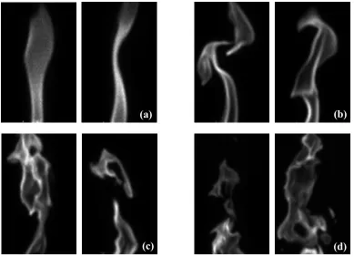
Figure 6: Unstable methane-air flame structure at (a) 4 atm, (b) 8 atm, (c) 16 atm, (d) 25 atm...18

Figure 7: Methane-air flame at 16 atm (frames from 12 second video clip)...19

Figure 8: Methane-air flame structure at (a) 1 atm, (b) 2 atm, (c) 25 atm ...22

Figure 9: Soot accumulated from high pressure ethylene-air flame...23

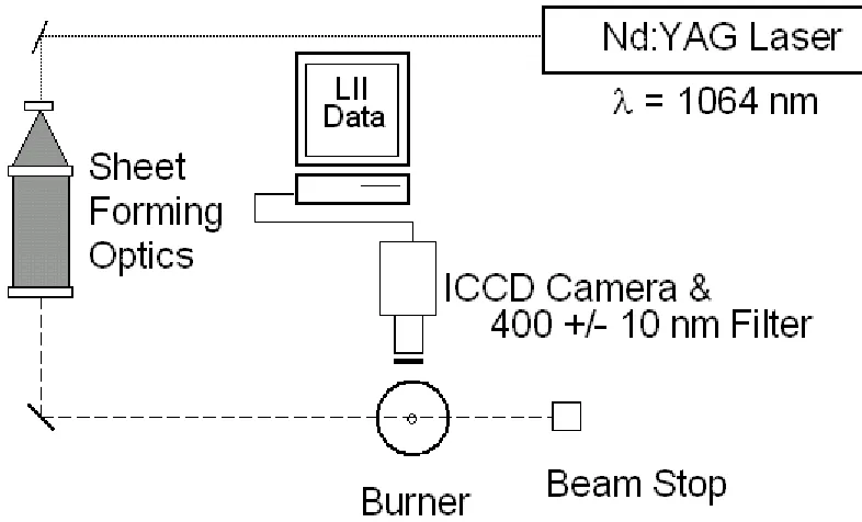
Figure 10: LII optical set-up ...25

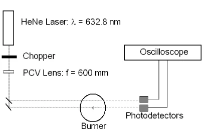
Figure 11: Optical schematic for extinction measurements...28

Figure 12: Path length of extinction measurement for methane-air and ethylene-air flames at 65% of 1 atm flame height on log-log scale...29

Figure 13: Transmission of laser extinction measurement at 65% of flame height at 1 atm ...30

Figure 14: Path averaged soot volume fraction versus pressure at 65% and 85% of the flame height at 1 atm...32

Figure 15: Path averaged soot volume fraction versus pressure on log-log scale ...33

Figure 16: Integrated fsv,ave versus pressure on a log-log scale for ethylene-air flames...34

Figure 17: Emissive power versus pressure on a log-log scale for a methane-air flame at pressures up to 50 atm (Miller & Maahs, 1977) ...35

Figure 18: Methane-air flame at (a) 2 atm and (b) 4 atm; scaled to maximum signal of 962 (red) ...36

Figure 19: Methane-air flame at (a) 8 atm, (b) 16 atm, (c) 25 atm; scaled to maximum signal of 6164 (red)...37

Figure 20: Ethylene-air flame at (a) 1 atm and (b) 2 atm; scaled to maximum signal of 1489 (red) ...37

Figure 21: Ethylene-air flame at (a) 4 atm, (b) 8 atm, and (c) 16 atm; scaled to maximum signal of 20703 (red)...38

Figure 22: Knife-edge device ...39

Figure 23: Energy distribution of laser sheet ...40

Figure 24: Decomposition of flame into J concentric rings (Choi & Jensen, 1998)...43

Figure 25: (a) Uncalibrated and uncorrected LII image and (b) calibrated and corrected LII image of ethylene-air flame at 16 atm...47

Figure 26: Soot volume fraction in methane-air flame at 2 atm...48

(7)

Figure 31: Soot volume fraction in ethylene-air flame at 1 atm...50

Figure 35: Calibrated and corrected LII images of methane-air flame normalized to maximum fsv of 25 atm case...53

(8)

1 Introduction

Because the overall equivalence ratio of combustion in a diffusion flame can be much lower than the premixed flammability limit, the fuel economy of a diffusion-flame-dominated device, such as a Diesel engine, is improved over that of a premixed-flame-device such as a homogeneous charge internal combustion engine. However, with this improvement in fuel economy comes the disadvantage of dramatically more soot production, which in turn causes increased soot loadings within the flame that affect the heat transfer characteristics of the flame, lowering the combustion efficiency. As soot is a sensitive indicator of the interactions between combustion chemistry and fluid mechanics, an examination of soot formation, especially at the elevated pressures that most practical combustion devices operate at in order to gain thermodynamic efficiency, will contribute to fundamental combustion knowledge.

1.1 Soot Formation

The formation of soot is the result of an ordered, but not fully understood, process. Efforts have been devoted to studying reaction mechanisms and chemical reaction pathways leading to the formation of soot (Frenklach, 2002; Richter & Howard, 2000). Before significant reductions in the amount of soot emitted from diffusion controlled combustion processes can be realized, more information about the soot formation process, particularly at physically relevant conditions, such as at elevated pressures, is required.

(9)

fundamental differences in the controlling mechanisms influencing each flame. A premixed hydrocarbon flame will yield soot if the flame system is deficient in oxidizer that is responsible for converting the hydrocarbon into CO and H2 (Wagner, 1981). It has been

experimentally shown that soot will be produced if the ratio of carbon to oxygen atoms, C/O, for the flame system is approximately greater than 0.5. If a non-soot-yielding ratio of C/O is maintained throughout the mixture region, soot will not be produced. In a diffusion flame, the combustion process is diffusion controlled as the fuel and oxidizer originate from different sides of the reaction zone; furthermore, in contrast to a premixed flame in which the fuel is heated in the presence of an oxidizer, in a diffusion flame the fuel undergoes thermally-induced decomposition or pyrolysis in the absence of an oxidizing species. Consequently, maintaining a non-soot-yielding ratio of C/O throughout the mixing region is very unlikely for a diffusion flame and soot formation is more prevalent in this type of flame.

As the parent fuel molecules are transported via diffusion into the preheat zone, the elevated temperatures cause the large molecules to thermally decompose into smaller hydrocarbon fragments. After the pyrolysis of a non-aromatic fuel, precursor monoelements, namely acetylene (C2H2), are formed. The amount of soot produced by a

given non-aromatic fuel is influenced by how easily the fuel can be converted to C2H2. For

(10)

with three C2H2 molecules combining into a benzene ring, C6H6. Several benzene rings

then group together generating polycyclic aromatic hydrocarbons (PAHs). The PAHs are multi-benzene ring structures, initially saturated. As these rings lose hydrogen atoms, which are oxidized to OH and eventually H2O, and become unsaturated, a process called

polymerization occurs and the ring structures begin to condense together. As polymerization continues, the ratio of carbon to hydrogen atoms increases and enough rings will eventually group together to form a small soot particle or spherule. Surface reactions on the spherule cause it to grow. For reasons still not understood, the spherules no longer grow after reaching diameters between 30 and 50 nm. The spherules then begin adhering together to form agglomerates. These agglomerates then combine to form clusters.

The formation of soot is countered by soot removal through oxidation. The oxidation of soot is observable in a simple candle flame. The yellow color of a candle is caused by the incandescence of hot soot. If the quality of the candle wax is high, most of the soot formed will be oxidized before diffusing across the flame front and the flame will not smoke. Carbon that is liberated from the flame is referred to in the literature as smoke while carbon that is oxidized within the flame is deemed soot. One of the early methods of examining soot formation in diffusion flames at elevated pressures was to observe what combination of fuel flow rate and pressure caused the flame to smoke, i.e. record the smoke point (McArragher & Tan, 1972).

(11)

composed of spherical particles arranged in roughly chain-like structures as shown in Figure 1. In fact, these agglomerates are fractal-like with a fractal dimension of approximately 1.8. The diameter of a spherical particle ranges from 10 to 200 nm, but the diameter is most commonly between 10 and 50 nm. The individual spherical particle is composed of approximately 104 crystallites, each of which consists of 5 to 10 sheets of carbon atoms. These sheets of carbon atoms have length and width dimensions of 2 to 3 nm and are made of approximately 100 carbon atoms (Palmer & Cullis, 1965).

Figure 1: Transmission electron micrograph of soot aggregates from ethylene counter-flow diffusion flame (Gaydon & Wolfhard, 1970)

(12)

in humans (Sydbom et al., 2001; Comstock et al., 1998; Morgan et al., 1997; Scheepers & Bos, 1992). Barfknecht (1983) details the historical progress of linking occupational soot exposure to its detrimental biological consequences. Additionally, Barfknecht examines the correlation between particulate air pollution levels and lung cancer mortality. This research indicates that polycyclic organic matter (POM), of which polycyclic aromatic hydrocarbons (PAHs) are a subset, is responsible for the mutagenic and carcinogenic properties of soot.

1.2 Effects of Elevated Pressure on Soot Formation

Most practical combustion devices operate at elevated pressures to increase thermodynamic efficiency, and consequently, it is important to examine the formation of soot under these conditions. It is well known that carbon formation increases while soot removal by oxidation declines with increasing pressure in diffusion-controlled devices (Flower & Bowman, 1986) and the rates of soot formation increase with increasing pressure (Flower, 1986). The mechanisms responsible for soot formation and oxidation at high pressures are significantly different than those active at low pressures. An exact, comprehensive explanation of these mechanisms and how they differ is still elusive, but it is generally agreed upon that elevating the pressure of a diffusion flame’s ambient environment causes changes in the diffusion coefficient and reaction rate, which lead to more soot being produced.

(13)

mass yield is soot volume fraction (fsv). Flower and Bowman (1986) made fsv

measurements in a laminar diffusion flame at elevated pressures up to 10 atmospheres using laser-scattering to examine the effects of pressure on soot formation and oxidation. The work of Flower and others indicates that increased pressure plays a significant role in increasing soot production in spray combustion, premixed flames, and diffusion flames (McArragher & Tan, 1972; Schalla & McDonald, 1955; Kadota et al., 1977; Miller & Maahs, 1977; Millberg, 1959; Fischer & Moss, 1998; Heidermann et al., 1999). Common diffusion-flame-devices operate at pressures between 25 and 30 atmospheres. The mechanisms responsible for soot formation at 1 or even 10 atmospheres may be drastically different than those prevailing at 30 atmospheres. Furthermore, Flower and Bowman collected line integrated fsv values, which do not provide spatially or temporally resolved

results. Tomography is one method that would provide spatially resolved fsv, but this

technique is limited in that it is time consuming and few high-pressure combustion devices provide the optical access required to employ tomography (Santoro & Shaddix, 2002).

(14)

1.3 Laser Diagnostic Techniques

1.3.1 Laser Extinction

Energy is removed from a beam of light, such as a laser beam, when the beam passes through a molecule- or particle-filled medium. The molecules or particles scatter and absorb light from the beam, causing the beam to attenuate. Scattering and absorption in combination represent the phenomena of extinction (Van de Hulst, 1957). Extinction measurements have been used to determine path averaged soot volume fraction, fsv,ave, and

physical properties of soot, such as particle diameter and cluster size and structure.

If soot particles are assumed to be within the Rayleigh-scattering regime (d << λ), the following relation may be used to calculate a path averaged fsv,ave (D’Alessio et al.,

1972)

{

(

1 )

/(

2 )

}

Im

)

/

ln(

6

2 2

,

+

−













=

m

I

L

f

o ave sv

π

λ

(1.1)

where I is the attenuated intensity, I0 is the unattenuated intensity, m is the index of

(15)

results by ± 40%. This particular index of refraction is generally accepted by the research community and was chosen so that comparisons could be drawn.

1.3.2 Laser Induced Incandescence

Laser Induced Incandescence (LII) capitalizes on soot primary spherules having diameters within the Rayleigh scattering regime and soot being an excellent absorber and, hence, emitter of radiation (Santoro & Shaddix, 2002). A brief, high energy laser pulse heats soot particles to near their vaporization temperature, ~ 4000 K, a temperature much greater than the temperature of the non-laser-heated soot within the flame, ~ 1800 K. Additionally, the wavelength of the thermal emission produced by the laser heated soot is blue-shifted in comparison to that of the non-laser-heated soot. The resulting incandescence can be collected by an intensified camera or other photodetecting device and used to determine qualitative and quantitative information about the soot field.

Over the last twenty years, the non-intrusive LII technique has proven itself to be a very versatile and important combustion diagnostic technique. Measurements of soot particle sizes (Bockhorn et al., 2002; Vander Wal et al., 1999; Starke & Roth, 2002; Will et al., 1995; Axelsson et al., 2000) and fsv (Quay et al., 1994; Vander Wal & Weiland, 1994;

(16)

(17)

2 Experimental Apparatus and Conditions

2.1 Co-flow Diffusion Flame Burner

The burner used in this work produces the classic over-ventilated Burke-Schumman (1928) laminar diffusion flame. The burner geometry and flow rates were modified several times to achieve a stable laminar flame. Methane and ethylene were used in the experiments with air as an oxidizer. Methane was chosen because it is a simple hydrocarbon and represents natural gas, which is a very important commercial fuel. Ethylene was selected because it is a larger hydrocarbon with a much higher tendency to form soot. Ethylene was chosen as the representative larger hydrocarbon instead of the more commonly used propane because propane has a very low saturation pressure at room temperature and liquefies at pressures even moderately above atmospheric.

2.1.1 Burner Geometry

(18)

was not influenced by the shear layer which forms between the co-flow and ambient air within the pressure vessel. Glass beads with a diameter of 4 mm filled the co-flow volume to aid in obtaining a uniform exit velocity profile. Steel wool was inserted in the fuel tube to create a pressure drop which made the fuel flow rate was less sensitive to pressure fluctuations upstream.

(19)

2.1.2 High Pressure Vessel

(20)

Figure 3: High pressure vessel

2.1.3 Ignition System

(21)

high temperature, high pressure epoxy. A piece of stripped, twisted copper wire (approximately 5 strands) was threaded through the ceramic tube and extended about 3 cm and 0.5 cm from each end respectively. The wires protruding were then sealed to the ceramic tube with high pressure gasket maker.

Figure 4: Ignition system electrode

(22)

Figure 5: Ignition system schematic

2.1.4 Flow and Pressure Control System

Four entry ports for gases existed on the pressure vessel. Two were located on the bottom of the pressure vessel and supply the burner’s fuel and air. The remaining two were located above two of the flanges housing windows and will hereafter be referred to as the “window ports.” Air was supplied to the window ports for the dual purposes of preventing soot and water condensation from accumulating on the windows and aiding in increasing the pressure within the vessel.

The air for both the burner and the window ports was supplied from four tanks of dry, hydrocarbon-free bottled air with a purity of 99.9%. During operation of the burner at elevated pressures, the pressure differential on the regulator was adjusted so as to remain approximately 50 psi greater than the pressure within the vessel. The supply line from the two-stage regulator was bifurcated with each branch leading to a separate Hastings Model

Transformer Battery

Switch

Electrode

(23)

201 flow meter with a 0-50 standard liter per minute (SLPM) range. The fuel flow rates required were much lower than those for the air supplies; thus the fuel flowed from the fuel bottle through a second two-stage regulator and a Hastings Model 200 flow meter with a 0-1000 standard cubic centimeter per minute (sccm) range. The purities of the methane and ethylene fuels were 99.0% and 99.5%, respectively. A Hastings Model 40 Power Supply provided both power to all three of the flow meters and a digital read-out of the flow rates for each meter. The flow meters were calibrated with nitrogen and thus a gas correction factor (GCF) was entered into the power supply for each gas. The GCFs provided by the manufacturer for air, methane, and ethylene were 0.9980, 0.7700, and 0.6040, respectively.

The fuel and air flow rates were kept constant as the pressure was increased within the vessel. For the methane-air flame at pressures ranging from 1 atm to 8 atm, the fuel flow rate was 0.100 SLPM, while the air flow rate was 20.0 SLPM. For the higher pressure flames, the fuel and air flow rates were increased to 0.150 SLPM and 30 SLPM in order to maintain an approximately constant flame height of 20 mm. The fuel and air flow rates for the ethylene-air flame were 0.060 SLPM and 20.5 SLPM, respectively. The value of the flow rates and the ratio of the fuel flow rate to the air flow rate greatly influenced the appearance and behavior of the flames, especially the stability as described in § 2.2.

(24)

the vessel (Appendix 8.2). In general the flow rate to the window ports was increased first, followed by slowly decreasing the exhaust flow rate to achieve a given pressure. If changes in the pressure differentials on the regulators were required, the adjustment was made prior to increasing the window ports’ flow rates. Great caution was exercised when making adjustments to any of the flow rates because operating under increased pressure made the flame more likely to suddenly extinguish. As the pressure was increased, reaction rates also increased while the diffusion rates remained relatively constant. The resulting flame had a thinner reaction zone and greater sensitivity to perturbations, i.e. if hydrodynamically disturbed, the flame was more likely to extinguish because diffusion of reactants cannot occur quickly enough to reestablish the flame (Miller & Maahs, 1977). The pressure within the vessel was displayed on an external gauge having a range of 0 to 1000 psig.

2.2 Physical Appearance of Flame

(25)

typical of laboratory flames that have been studied by others and offers better spatial resolution of the soot field. As the pressure was increased, the flow rates of the fuel and air were raised as well to maintain the constant flame height. At pressures nearing 25 atm, the velocity matched fuel and air flow rates were 1.0 SLPM and 71.43 SLPM. Under these conditions, the flame maintained a constant height and had velocity matched flow rates, but it was very unstable at pressures greater than 4 atm as depicted in Figure 6.

Figure 6: Unstable methane-air flame structure at (a) 4 atm, (b) 8 atm, (c) 16 atm, (d) 25 atm

At pressures of 1 atm and 2 atm, the flame maintained the conventional over-ventilated, candle flame-like shape. Above 2 atm, the flame began to wrinkle and the

(a) (b)

(26)

flame front was significantly contorted. Flame pockets began to break from the primary flame as shown in Figure 7. This figure shows six frames from a video of a methane-air flame operating at 16 atm. The vortical shapes and pocket formations are very prominent.

Figure 7: Methane-air flame at 16 atm (frames from 12 second video clip)

(27)

Flower & Bowman (1986) and Miller & Maahs (1977) have done the majority of research on soot production in laminar diffusion flames at elevated pressures. As stated in § 1.2, the work of Flower & Bowman was performed up to a maximum pressure of 10 atm and evaluated an ethylene-air flame. To achieve a stable, axisymmetric flame at pressures greater than 2 atm, Flower and Bowman used fuel flow rates ranging from 0.102 to 0.294 SLPM, with an air flow rate of 252 SLPM at 1 atm (Flower & Bowman, 1986). The fuel flow rates used by Flower and Bowman were much lower than those used to generate the previously discussed unstable flame in the present work, and the air flow rate was significantly greater. Flower & Bowman described their flame as being “greatly overventilated” and stated that “this air flow is 60 times the stoichiometric requirement for the highest fuel flows studied.” It was theorized that this overventilation helped to maintain a stable flame structure, but unfortunately, with the air flow meters and air supply system used in this work such high air flow rates could not be achieved, particularly at higher pressures. This proposed connection between extreme overventilation and flame stability was further supported by the work of Miller and Maahs (1997), who studied nitrogen oxide (NOx) formation in a laminar methane-air diffusion flame at pressures up to

(28)

Beginning with the relationship between the fuel and air flow rates used by Miller and Maahs and experimenting with the burner of the present work, it was determined that for the methane-air flame to remain stable at pressures approaching 25 atm, the air flow rate needed to be 20 SLPM, or 2.8 times the air flow rate required to match the velocity of a 0.1 SLPM methane flow rate. Similarly for the ethylene-air flame, it was determined that an air flow rate of 20.5 SLPM, 4.7 times the air flow rate required to match the velocity of a 0.06 SLPM ethylene flow rate, would produce a stable flame.

Observations on the effects of pressure on the physical characteristics of the flame were similar to those made by Miller and Maahs (1977). In their work, they also noted that the flame was wide and convex at 1 atm, and as the pressure increased, the flame became thinner and more concave. It was also observed that the naturally occurring soot incandescence increased with pressure. Figure 8 shows the flame at 1, 4 and 25 atm. The blue zone is indicative of O2 Schumann-Runge radiation and CO + O continuum radiation

while the brighter blue zones on the sides and near the fuel tube is evidence of C2 and CH

(29)

atmospheric pressure, which may explain the significant change in flame shape with increasing pressure; comparatively, soot particles are higher in mass than other combustion products and cannot diffuse away from the primary flame region as a gaseous product might. Combustion must then be maintained by oxygen diffusing inward to the primary flame region, resulting in a narrowing flame structure (Miller & Maahs, 1977).

Figure 8: Methane-air flame structure at (a) 1 atm, (b) 2 atm, (c) 25 atm

The fuel and air flow rates also influenced the height of the flame. The flow rates chosen to ensure flame stability resulted in a flame height of approximately 20 mm or 5 times the inside diameter of the fuel tube.

As expected, the ethylene-air flame produced much more soot than the methane-air flame. This was evident in the flame appearance, as the orange color associated with soot incandescence appeared in a greater portion of the ethylene-air flame than in the methane-air flame at a given pressure. As discussed in § 2.4, the transmission of the extinction laser beam decreased more dramatically with increasing pressure for the ethylene-air flame. In

(30)

the ethylene-air flame at pressures of 16 atm and above, soot accumulated around the fuel tube exit (Figure 9). As a consequence, no LII data was taken for the ethylene-air flame above 16 atm.

Figure 9: Soot accumulated from high pressure ethylene-air flame

2.3 Laser Induced Incandescence

Spatially and temporally resolved measurements of fsv are desired in order to

determine such physical processes as the rates of primary particle formation, clustering, cluster-cluster agglomeration, and oxidation in diffusion flames. To obtain spatially resolved, instantaneous fsv measurements, Laser Induced Incandescence (LII) is employed.

(31)

measurements. An operating procedure for the combined use of the burner and LII technique is given in Appendix 8.3.

2.3.1 Optical Set-up

(32)

Figure 10: LII optical set-up

(33)

2.3.2 Timing and Wiring

A SRS DG-535 digital delay generator served as the master clock for the LII measurements and provided TTL signals to the laser that commanded a given laser event, such as flash lamp or Q-switch activation (Appendix 8.4). The internal trigger of the DG-535 was set at 10 Hz. This repetition rate was chosen because the Nd:YAG laser operates between 8 and 15 Hz. Thus a command, T0, was sent to the laser flash lamps at an

approximate rate of 10 Hz. The laser Q-switch was activated 160 µsec after the flash lamps (positive going AB TTL = T0 + 160 µsec). The DG-535 also triggered the Princeton

Instruments PG-200, the camera gate controller, at 150 µsec after a flash lamp signal (positive going CD TTL = T0 + 150 µsec); the PG-200 then activated the Princeton

(34)

overlap of laser and acquisition events. A gate width of 30 ns was used in the present work. DeCroix and Roberts (2000) found that a gate width of 30 ns provided acceptable signal-to-noise ratios for even the low soot yielding methane-air flames without biasing the data towards larger particles; the larger particles cool more slowly than smaller particles that have a larger surface area to volume ratio. The LII signal of smaller particles decays more quickly.

2.4 Extinction Measurements

(35)

the considerable influence of flame luminosity on the collected signal. An oscilloscope then digitized and temporally averaged the signal collected by the photodiodes.

Extinction measurements were taken for both methane-air and ethylene-air flames at approximately 65% of the 1 atm flame height or 10 mm above the burner for the second set of experiments when the flame was stable and shortened in height. Additional extinction measurements were taken with the methane-air flame at 85% of the flame height.

Figure 11: Optical schematic for extinction measurements

(36)

were taken with the intensified camera. The exact pixel location of the laser beam’s passing was known and the path length was measured at that height. As Figure 12 shows, the path length decreased with increasing pressure, indicative of the narrowing effects pressure has on flame shape. The path length of the methane-air flame scaled with pressure as p-0.46 and the path length of the ethylene-air flame as p-0.57.

Log (Pressure) L o g (P a th L e ngt h)

0 0.2 0.4 0.6 0.8 1

0 0.1 0.2 0.3 0.4 0.5 0.6 0.7 0.8 0.9 1 Methane Ethylene

Figure 12: Path length of extinction measurement for methane-air and ethylene-air flames at 65% of 1 atm

(37)

The extinction measurements were taken at pressures of 1, 2, 4, 6, 8 and 10 atm. Above this pressure, both the methane-air and the ethylene-air flames are no longer considered “optically thin,” i.e., the transmission of the laser beam approaches or drops below 80%. As Figure 13 shows, the ethylene-air flame rapidly deviates from the condition of being optically thin above pressures of 2 atm.

Pressure (atm)

T

ra

n

sm

issi

o

n

(I

/I0

)

0 2 4 6 8 10

0 0.1 0.2 0.3 0.4 0.5 0.6 0.7 0.8 0.9 1

Methane Ethylene

(38)

3 Extinction Measurements and Soot Volume Fraction

3.1 Extinction Measurements as Calibration

The calibration procedure requires measuring the extinction ratio of a second lower-powered laser, knowing an accurate path length, and assuming an axisymmetric flame. The extinction ratio is the ratio of the signal of the attenuated beam to the signal of the unattenuated beam. The attenuated beam passes through the flame while the unattenuated beam does not. It is desired to use an extinction ratio that corresponds to an optically thin flame as described in § 2.4. The outcome of the calibration procedure is a calibration factor that relates LII signal intensity to soot volume fraction and ultimately leads to a quantitative image of fsv throughout the flame (Choi & Jensen, 1998; DeCroix & Roberts, 2000). This

correction factor found at a pressure yielding an optically thin flame can then be applied to the LII images taken at other pressure cases up to 25 atm.

3.2 Soot Volume Fraction

The extinction measurements collected for the calibration procedure were also used to calculate path averaged fsv,ave values at the height above the burner where the extinction

measurement was taken as described in § 1.3.1. The majority of previous fsv,ave data taken

at elevated pressures has been data of this nature. For comparison, these path averaged

fsv,ave values were calculated for the methane-air flame at 65% and 85% of the flame height

(39)

path length was measured from images of the flame taken simultaneously with the extinction measurements.

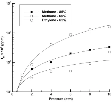
Pressure (atm)

fsv

x1

0

6 (ppm)

0 2 4 6 8 10

100 101 102 103

Methane - 85% Methane - 65% Ethylene - 65%

Figure 14: Path averaged soot volume fraction versus pressure at 65% and 85% of the 1 atm

flame height

When fsv,ave is plotted versus pressure on a log-log scale (Figure 15), the slope of the

(40)

fsv,ave∝ pm, where m is the slope of the linear fit. For the methane-air flame at 85% of the

flame height, m = 1.1; the methane-air flame at 65% of the flame height, m = 0.77; and the ethylene-air flame at 65% of the flame height, m = 1.75.

Log (Pressure)

Log

(fsv

x1

0

6 )

0 0.2 0.4 0.6 0.8 1

0 1 2 3

Methane - 85% Methane - 65% Ethylene - 65%

Figure 15: Path averaged soot volume fraction versus pressure on log-log scale

(41)

ethylene-air flames with a fuel flow rates of 1.7 scc/s, 2.4 scc/s and 3.9 scc/s. The fsv,ave

values measured in the present work’s ethylene-air flame, which has a fuel flow rate of 1.0 scc/s, were integrated and plotted along with the results of Flower and Bowman (1986) in Figure 16. The integrated fsv,ave values shown in Figure 16 were found at the same

non-dimensional axial location. The integrated fsv,ave for the ethylene-air flame of the present

work scaled with pressure as p1.2. The integrated fsv,ave values of Flower and Bowman at

1.7 scc/s, 2.4 scc/s and 3.9 scc/s scaled as p1.2, p1.1 and p1.0, respectively.

Log (Pressure) Log (I n te g ra te d

fsv,

a

ve

)

0 0.2 0.4 0.6 0.8 1

0 0.25 0.5 0.75 1 1.25 1.5 1.75 1.0 scc/s

Flower & Bowman - 1.7 scc/s Flower & Bowman - 2.4 scc/s Flower & Bowman - 3.9 scc/s

Figure 16: Integrated fsv,ave versus pressure on a

(42)

Some similar comparisons can be made with the work of Miller and Maahs (1977). While they did not explicitly measure fsv,ave, they did measure the emissive power from the

flame at pressures up to 50 atm. As shown in § 2.2, increasing luminosity is indicative of increasing soot presence within a flame. In examining Figure 17, it becomes evident that two pressure trends are present. The emissive power of the methane-air flame scaled as p1.4 for pressures between 0 and 25 atm. As the pressure was increased above pressures of 25 atm, the emissive power and consequently fsv,ave have a decreased dependence on pressure,

p0.2.

Log (Pressure)

Log

(E

mi

ss

iv

e

P

ow

e

r)

0.5 1 1.5 2

2.5 3 3.5 4

Figure 17: Emissive power versus pressure on a log-log scale for a methane-air flame at pressures

(43)

4 Calibration of LII Measurements

4.1 Correction of Raw LII Signal

Before the calibration procedure began, the raw LII signals were corrected for both background noise and variations in the energy distribution of the laser sheet. Figures 18 through 21 show the uncorrected LII signals for the methane-air and ethylene-air flames at various pressures with the laser sheet moving from left to right. The effect of pressure on soot production is even evident in these uncorrected and uncalibrated images. The images are colored according to the signal value of each pixel. Note that the lower pressure cases are colored according to different scales as the change in signal values is so dramatic with increasing pressure – one order of magnitude for the methane-air flame and two orders of magnitude for the ethylene-air flame.

Figure 18: Methane-air flame at (a) 2 atm and (b) 4 atm; scaled to maximum signal of 962 (red)

(44)

Figure 19: Methane-air flame at (a) 8 atm, (b) 16 atm, (c) 25 atm; scaled to

maximum signal of 6164 (red)

Figure 20: Ethylene-air flame at (a) 1 atm and (b) 2 atm; scaled to maximum signal of 1489 (red)

(a) (b) (c)

(45)

Figure 21: Ethylene-air flame at (a) 4 atm, (b) 8 atm, and (c) 16 atm; scaled to maximum signal

of 20703 (red)

4.1.1 Background Noise

Variation in the camera dark current intensity was the only major source of background noise, as flame luminosity as a source of background noise was largely removed by using a narrow bandpass filter. The camera dark current intensity was a function of CCD temperature, which varies somewhat because the temperature of the ground water used for cooling is not constant. To account for the variations in dark current intensity, a set of 10 images were taken with the camera lens capped prior to any collection of LII data. These 10 images were then averaged and subtracted from the LII images.

(46)

4.1.2 Laser Sheet Energy Distribution

The distribution of energy through the laser beam is non-uniform and usually follows a Gaussian profile. When this nominally round beam is collapsed in one direction to form a sheet, the Gaussian profile becomes even steeper. To correct for this variation in energy distribution, a knife-edge with a precise translation device was fixed above the center of the fuel tube (Figure 22).

Figure 22: Knife-edge device

(47)

beam was fully blocked. From the energy meter readings, a profile of the energy distribution of the laser sheet was determined. Several series of readings were taken and averaged to give the profile shown in Figure 23. Since the laser energy was not uniform across the sheet, different areas of the flame experienced variations in heating due to the laser. To correct the LII images for this discrepancy, each column of the LII image was divided by the profile shown in Figure 23.

Normalized Signal

D

is

ta

n

ce

a

bov

e

bur

n

e

r

(mm

)

0 0.2 0.4 0.6 0.8 1

0 5 10 15 20 25 30 35 40

(48)

4.2 Calibration Methodology

(49)

right side and the direction of the laser propagation is left to right. Thus the calibration factor found using traditional calibration techniques is erroneous as it is based on a projected LII intensity. Shaddix and Smyth (1996) report that corrections for signal trapping and laser sheet attenuation are necessary in flames with soot loadings greater than 1 ppm. The flames studied in this work have soot loadings well above 1 ppm. A calibration methodology developed by Choi and Jensen (1998) accounts for both signal trapping and laser energy sheet losses. This methodology uses the unattenuated signal and yields a soot concentration calibration factor that is only influenced by the LII optical system and not by the amount of soot contained within the flame.

The methodology developed by Choi and Jensen (1998) and utilized with experimental data by DeCroix and Roberts (2000) will be discussed briefly. Figure 24 shows the top view of a typical axisymmetric diffusion flame that has been decomposed into J concentric circles. The center of the rings is positioned at the centerline of the flame. The rings are located at the midpoint of adjacent pixels, ∆x/2, in the LII image; the last ring was located at the pixel corresponding to the edge of the flame. The laser sheet used for LII measurements would pass through the flame at y=0, perpendicular to the x-y plane, and in the direction of the x-axis. The attenuated intensity projected from the laser sheet location (y=0) to the camera detector is Ip. The Ip(j) shown in Figure 24 is the projected LII

intensity at x=j; it is the goal of the calibration methodology to correct this Ip to an

unattenuated intensity, I. The value yj,j+1 is the chordlength (beginning at the edge of the

(50)

route to the camera detector. Each chordlength, yj,j, is determined from trigonometry and is

identical to a pathlength that would yield a soot volume fraction fsv(j).

Y

X

Laser Sheet

I

_p

(j)

Detector

0 1 2 j

J

y_j,,j

y_j,j+1

y_j,J

Y

X

Laser Sheet

I

_p

(j)

Detector

0 1 2 j

J

y_j,,j

y_j,j+1

y_j,J

Figure 24: Decomposition of flame into J concentric rings (Choi & Jensen, 1998)

(51)

                  ⋅ =

∑

= λ π J j

i sv ji

p y j f m E j I j I , ) ( ) ~ ( 6 exp ) ( )

( (4.1)

where λ is the detection wavelength and

» ¼ º « ¬ ª + − − = 2 ~ 1 ~ Im ) ~

( ₂2

m m m

E (4.2)

where m~ is the index of refraction of soot and taken to be 1.57-i0.56 for reasons discussed in § 1.3.1. Since Choi and Jensen’s calibration factor, CF, provides a relationship between I and fsv, equation 4.1 can be rewritten as

                  ⋅ = =

∑

= λ π J j i i j sv p sv y j f m E j I CF j f j I , ) ( ) ~ ( 6 exp ) ( ) ( )

( (4.3)

The unknowns in equation 4.3 are fsv(j) and CF. If the value for CF is known,

equation 4.3 can be iteratively solved at each pixel marching from j=J-1 to j=0. The collected LII signal at the outer edge of the flame can be assumed to be unattenuated since it does not pass through a soot field en route to the camera detector nor has the laser sheet been attenuated by any soot field within the flame; thus, I(J)=Ip(J).

(52)

                    ⋅ ∆ + ⋅ ∆ + ⋅ ∆ − =    

∑

− = λ π 1 1 0 ) ( ) ( 2 ) 0 ( ) ~ ( 6 exp J j sv sv sv p J f x j f r f x m E I I (4.4)

where ∆x is the spacing between concentric rings. The predicted transmission was then compared to the experimental transmission found through laser light extinction measurements described in § 2.4. A new guess for the calibration factor was chosen and equations 4.3 and 4.4 were solved iteratively until a calibration factor was converged upon. DeCroix wrote a FORTRAN program that uses this iterative approach to find a calibration factor and corrected fsv profile. The program was extensively tested with artifical soot

volume fraction profiles; the methodology, source code and verification of the code are available in the dissertation of DeCroix (1998). The programs written by DeCroix were used to find the calibration factors and generate corrected images for the diffusion flames investigated in this work.

(53)

4.3 Calibration of LII Images

(54)

Figure 25: (a) Uncalibrated and uncorrected LII image and (b) calibrated and corrected LII image

of ethylene-air flame at 16 atm

Figure 26Figure 34 show the measured fsv in the flame at increasing pressures using

methane and ethylene as fuels. In each of these images, the color scale representative of fsv

in parts per million (ppm) is not normalized, i.e., each image is scaled to its particular maximum fsv. The influence of fuel type on soot yield is apparent in these images as the

ethylene-air flame has a higher soot volume fraction than the methane-air flame at a given pressure.

(55)

Figure 26: Soot volume fraction in methane-air flame at 2 atm

Soot Volume Fraction

3 ppm

0 ppm

5 ppm

(56)

20 ppm

0 ppm

30 ppm

(57)

Figure 31: Soot volume fraction in ethylene-air flame at 1 atm

40 ppm

0 ppm

3 ppm

(58)

10 ppm

0 ppm

55 ppm

(59)

As pressure increases, the regions of high soot yield shift. This can be observed when comparing the methane-air flame at 8 atm (Figure 28) and 25 atm (Figure 30). At 8 atm, the peak sooting regions are located on the sides of the flame, and as the pressure increases to 25 atm, the tip of the flame becomes the highest sooting region. Figures 35 and 36 give more striking views of the effects of pressure on soot production and flame shape. These calibrated LII images have been normalized to the highest sooting case – 25 atm for the methane-air flame and 16 atm for the ethylene-air flame. When shown on the same scale as the highest pressure case, the soot field for the lowest pressure case is hardly distinguishable. These images also reiterate the physical changes the flame undergoes with increasing pressure, namely a significant narrowing of the flame.

300 ppm

(60)

0 ppm 40 ppm

Figure 35: Calibrated and corrected LII images of methane-air flame normalized to maximum fsv

of 25 atm case

0 ppm 300 ppm

Figure 36: Calibrated and corrected LII images of ethylene-air flame normalized to maximum fsv

of 16 atm case

2 atm 4 atm 8 atm 16 atm 25 atm

2 atm 4 atm 16 atm

(61)

5 Conclusions

A better understanding of the formation of soot is desired in order to gain a more comprehensive picture of combustion processes and to reduce the resulting emission of soot particulates into the environment. Examining soot at elevated pressures is especially relevant as most work-producing devices operate at high pressures in order to gain thermodynamic efficiency. The present work has explored the formation of soot at elevated pressures up to 25 atm in a methane-air co-flow diffusion flame and up to 16 atm in an ethylene-air co-flow diffusion flame. The non-intrusive LII diagnostic technique was employed to gain spatially and temporally resolved measurements of the soot volume fraction. This research is unique in that it represents the first time that spatially and temporally resolved measurements of soot volume fraction in a diffusion flame have been taken at elevated pressures up to 25 atm. The conclusions obtained from this research are listed below.

Path Averaged ffffsv

1.) The pressure dependences of the path averaged fsv for the methane-air and

ethylene-air flames are found to be P0.65 and P1.7, respectively.

2.) The path averaged fsv for the ethylene-air flame compares well with published

results. There are no previously published methane-air flame measurements of

(62)

Physical Characteristics of Flame

1.) Methane-air and ethylene-air flames are no longer optically thin above 8 atm and 2 atm, respectively, indicating that the path averaged fsv measurements made

above these pressures are questionable.

2.) Flame structure changes dramatically with increasing pressure. With velocity matched fuel and air flow rates that produce a flame with a height of 60 mm, the flame becomes very contorted and profoundly influenced by buoyancy-driven instabilities.

3.) A greatly over-ventilated flame is required for flame stability at elevated pressures. The fuel and air flow rates are not velocity matched in this case and a flame with an approximate height of 20 mm is used.

4.) The physical shape of the flame is very sensitive to increases in pressure. The flame becomes shorter in height and considerably narrower with increasing pressure. The path length of the methane-air flame scales with pressure as p-0.46 and the path length of the ethylene-air flame as p-0.57. The region of the flame responsible for precursor formation also becomes narrower.

Spatially and Temporally Resolved ffffsv

(63)

2.) Peak fsv pressure dependence for the methane-air flame is p1.2 and for the

ethylene-air flame is p1.7, which varies from the path averaged fsv pressure

dependence.

3.) The region of peak fsv shifts from the wings of the flame to the tip with

(64)

6 Future Work

(65)

7 References

Axelsson, B., Collin, R., and Bengtsson, P., “Laser-induced incandescence for soot particle size measurements in premixed flat flames,” Appl. Opt. 39, 3683-3690 (2000).

Axelsson, B., Collin, R., and Bengtsson, P. E., “Laser-induced incandescence for soot particle size and volume fraction measurements using on-line extinction calibration,” Appl. Phys. B 72, 367-372 (2001).

Barfknecht, T. R., “Toxicology of soot,” Prog. Energy Combust. Sci. 9, 199-237 (1983).

Bockhorn, H., Geitlinger, H., Jungfleisch, B., Lehre, Th., Schön, A., Streibel, Th., and Suntz, R., “Progress in characterization of soot formation by optical methods,” Phys. Chem. Chem. Phys. 4, 3780-3793 (2002).

Bohren, C. F. and Huffman, D. R., Absorption of Scattering of Light by Small Particles, Wiley, 1983.

Bryce, D. J., Ladommatos, N., and Zhao, H., “Quantitative investigation of soot distribution by laser-induced incandescence,” Appl. Opt. 39, 5012-5022 (2000).

Burke, S. P. and Schumann, T. E. W., “Diffusion flames,” Proceedings of the First and Second Symposium on Combustion, The Combustion Institute, 2-11 (c.1965).

Choi, M. Y. and Jensen, K. A., “Calibration and correction of laser-induced incandescence for soot volume fraction measurements,” Combust. Flame 112, 485-491 (1998).

Comstock, M. L., “Diesel exhaust in the occupational setting – Current understanding of pulmonary health effects,” Clinics in Lab. Med. 18, (1998).

(66)

Dalzell, W. H. and Sarofim, A. F., “Optical constants of soot and their application to heat-flux calculations,” J. Heat Transfer 91, 100 (1969).

DeCroix, M. E., “The effects of unsteady hydrodynamics on soot formation in a counterflow diffusion flame,” NC State University, Dissertation (1998).

DeCroix, M. E. and Roberts, W. L., “Transient flow field effects on soot volume fraction in diffusion flames,” Combust. Sci. Tech. 160, 165-189 (2000).

Eckbreth, A. C., “Effects of laser-modulated particulate incandescence on Raman scattering diagnostics,” J. Appl. Phys. 48, 4473-4479 (1977).

Fischer, B. A. and Moss, J. B., “The influence of pressure on soot production and radiation in turbulent kerosine spray flames,” Combust. Sci. and Tech. 138, 43-61 (1998).

Flower, W. L. and Bowman, C. T., “Measurements of the effect of elevated pressure on soot formation in laminar diffusion flames,” Combust. Sci. and Tech. 37, 93-97 (1984).

Flower, W. L. and C. T. Bowman, “Soot production in axisymmetric laminar diffusion flames at pressures from one to ten atmospheres,” Twenty-first Symposium

(International) on Combustion, The Combustion Institute, 1115-1124 (1986).

Flower, W. L., “The effect of elevated pressure on the rate of soot production in laminar diffusion flames,” Combust. Sci. and Tech. 48, 31-43 (1986).

Flower, W. L., “Observations on the soot formation mechanism in laminar ethylene-air diffusion flames at one and two atmospheres,” Combust. Sci. and Tech. 53, 217-224 (1987).

Frenklach, M., “Reaction mechanisms of soot formation inflames,” Phys. Chem. Chem. Phys. 4, 2028-2037 (2002).

(67)

Glassman, I., Combustion, 2nd ed., Harcourt Brace Jovanovich: New York, 1987.

Heidermann, T., Jander, H., and Wagner, H. G., “Soot particles in premixed C2H4-air

flames at high pressures (P=30-70 bar),” Phys. Chem. Chem. Phys. 1, 3497-3502 (1999).

Hu, D., Braun-Unkhoff, M., and Frank, P., “Modeling study on initial soot formation at high pressures,” Zeitschrift fur Physikalische Chemie 214, 473-491 (2000).

Jost, Wilhelm, trans. by Huber Croft, Explosion and Combustion Processes in Gases, 1st ed., McGraw-Hill: New York, 1946.

Kadota, T., Hiroyasu, H., and Farazandehmer, A., “Soot formation by combustion of a fuel droplet in high pressure gaseous environments,” Combust. Flame 29, 67 (1977).

Kazakov, A., Wang, H., and Frenklach, M., “Detailed modeling of soot formation in laminar premixed ethylene flames at a pressure of 10 bar,” Combust. Flame 100, 111-120 (1995).

Li, Y., “Applications of Transient Grating Spectroscopy to Temperature and Transport Properties Measurements in High-Pressure Environments,” NC State University, Dissertation (2001).

McArragher, J. S. and Tan, K. J., “Soot formation at high pressure: a literature review,” Combust. Sci. Tech. 5, 257 (1972).

Melton, L. A., “Soot diagnostics based on laser heating,” Appl. Opt. 23, 2201-2208 (1984).

Millberg, M. E., “Carbon formation in an acetylene-air diffusion flame,” J. Phys. Chem.

63, 578 (1959).

(68)

Miller, I. M. and Maahs, H. G., “Effect of pressure on structure and NOx formation in

CO-air diffusion flames,” NASA TN D-1448 (1979).

Miller, I. M. and Maahs, H. G., “Pollutant emissions from flat-flame burners at high pressures,” NASA TN D-1673 (1980).

Morgan, W. K. C., Reger, R. B., and Tucker, D. M., “Health effects of diesel emissions,” Ann. Occup. Hyg. 41, 643-658 (1997).

Palmer, H. B. and Cullis, H. F., The Chemistry and Physics of Carbon, vol. 1, Marcel Dekker: New York, 1965.

Parker, W. G. and Wolfhard, H. G., “Carbon formation in flames,” J. Chem. Soc., 2038-2049 (1950).

Quay, R., Lee, T., Ni, T., and Santoro, R. J., “Spatially resolved measurements of soot volume fraction using laser-induced incandescence,” Combust. Flame 97, 384-392 (1994).

Richter, H. and Howard, J. B., “Formation of polycyclic aromatic hydrocarbons and their growth to soot – a review of chemical reaction pathways,” Prog. Energy Combust. Sci.

26, 565-608 (2000).

Santoro, R. J. and Shaddix, C. R., “Laser-induced incandescence,” Applied Combustion Diagnostics. Taylor & Francis: New York, 2002.

Schalla, R. L. and McDonald, G. E., “Mechanisms of soot formation in diffusion flames,” Fifth Symposium (International) on Combustion, The Combustion Institute, Pittsburgh, 316 (1955).

(69)

Schittkowski, T., Mewes, B., and Bruggemann, D., “Laser-induced incandescence and Raman measurements in sooting methane and ethylene flames,” Phys. Chem. Chem. Phys. 4, 2063-2071 (2002).

Shaddix, C. R. and Smyth, K. C., “Laser-induced incandescence measurements of soot production in steady and flickering methane, propane, and ethylene diffusion flames,” Combust. Flame 107, 418-452 (1996).

Starke, R. and Roth, P., “Soot particle sizing by LII during shock tube pyrolysis of C6H6,”

Combust. Flame 127, 2278-2285 (2002).

Sydbom, A., Blomberg, A., Parnia, S., Stenfors, N., Sandstrom, T., and Dahlen, S. E., “Health effects of diesel exhaust emissions,” European Respiratory J. 17, 733-746 (2001).

Van de Hulst, H. C., Light Scattering by Small Particles, Dover: New York, 1957.

Vander Wal, R. L. and Weiland, K. J., “Laser-induced incandescence: Development and characterization towards a measurement of soot-volume fraction,” Appl. Phys. B 59, 445-452 (1994).

Vander Wal, R. L., Choi, M. Y., and Lee, K., “The effects of rapid heating of soot: Implications when using laser-induced incandescence for soot diagnostics,” Combust. Flame 102, 200-204 (1995).

Vander Wal, R. L., Zhou, Z., and Choi, M. Y., “Laser-induced incandescence calibration via gravimetric sampling,” Combust. Flame 105, 462-470 (1996).

Vander Wal, R. L., “Laser-induced incandescence: detection issues,” Appl. Opt. 35, 6548-6559 (1996).

(70)

Vander Wal, R. L. and Ticich, T. M., “Cavity ringdown and laser-induced incandescence measurements of soot,” Appl. Opt. 38, 1444-1451 (1999).

Vander Wal, R. L., Ticich, T. M., and Stephens, A. B., “Can soot primary particle size be determined using laser-induced incandescence?” Combust. Flame 116, 291-296 (1999).

Wagner, H. G., Seventeenth Symposium (International) on Combustion, The Combustion Institute, Pittsburgh, 3 (1979).

Wagner, H. G., ed. by D. Siegla & G. Smith, “Soot formation – an overview,” Particulate Carbon: Formation During Combustion, Plenum: New York, 1981.

Welle, E., “The frequency response of counterflow diffusion flames,” NC State University, Dissertation (2002).

Will, S., Schraml, S., and Leipertz, A., “Two-dimensional soot-particle sizing by time-resolved laser-induced incandescence,” Opt. Lett. 20, 2342-2344 (1995).

(71)

8 Appendices

8.1 Pressure Vessel Window Assembly

The pressure vessel windows should be cleaned with alcohol. Prior to reinstalling the cleaned windows, a thin layer of vacuum grease should be applied to the circumference of the window and the inside surfaces of the window’s Teflon holder. The window should then be carefully pressed into the Teflon holder. The Teflon holder is then inserted into the middle flange as shown below.

Pressure Vessel

Window with Teflon Holder

(72)

8.2 Pressure Build-up Methodology

The exhaust flow of the high pressure vessel is controlled by a needle value. Approximately five and one half turns fully closes the valve. While trying to maintain a flame within the pressure vessel, it is imperative that the needle valve never be fully closed as the flame will without exception extinguish. The following two tables show the methodologies for maintaining a methane-air flame up to a pressure of 25 atm and an ethylene-air flame up to a pressure of 16 atm.

Pressure

(atm) Methane (slpm) Co-flow Air (slpm) Window Port Air (slpm)

Total Downward

Turns of Needle

Valve

1 0.10 20.0 10.0 0.00 2 0.10 20.0 25.5 3.50 4 0.10 20.0 40.0 4.50 8 0.10 20.0 85.0 4.75

16 0.15 30.0 110.0 5.00

25 0.15 30.0 110.0 5.10

Pressure

(atm) Ethylene (slpm) Co-flow Air (slpm) Window Port Air (slpm)

Total Downward

Turns of Needle

Valve

1 0.06 20.5 10.0 0.00 2 0.06 20.5 30.0 3.50 4 0.06 20.5 45.0 4.75 8 0.06 20.5 85.0 5.00

(73)

8.3 LII Measurments: Operating Procedure

1.) Turn on Hastings Model 40 Power Supply for the flow meters and allow to warm up for one hour.

2.) Turn on N2 to camera. Wait 15 minutes.

3.) Turn on water to camera and pressure vessel. Wait 10 minutes

4.) Turn on detector controller (two switches). Wait 10 minutes after green light has come on.

5.) Meanwhile, set flow rates for fuel and air.

6.) Turn on PG-200, Signal Delay Generator DG 535, Oscilloscope, Photodetector, Laser and computer.

7.) Take flat field images with camera lens capped.

8.) Remove camera lens cover and attach filter (mirror-like side facing away from the flame).

9.) Remove plastic coverings from optics.

10.) Open both exhaust needle valve and two-way valve fully. (Burner will not ignite with two-way valve closed.)

11.) Light Burner. (Turn on fuel to burner. Immediately light burner. Turn on air to burner. Turn on air to window ports.)

12.) Turn on exhaust fan.

13.) Slowly close two-way valve.

14.) Turn on laser with appropriate beam dump in place. 15.) Collect images using IPLab software.

When finished collecting data, turn fuel off at bottle and allow excess fuel in fuel line to burn away. Then turn off air supplies and equipment. Turn off water to camera and allow the N2 to flow for 10-15 minutes before turning off as well. Cover optics and turn off

(74)