ABSTRACT
LOU, JIALIN. Development and Implementation of Reconstructed Discontinuous Galerkin Methods for Computational Fluid Dynamics on GPUs. (Under the direction of Hong Luo.)
Recently, the application of general-purpose graphics processing unit (GPGPU) technology to the computational fluid dynamics (CFD) solvers has been popular. With GPGPU, one can benefit from an exciting opportunity to significantly accelerate the CFD solvers by offloading the compute-intensive portions of the application to the GPU, while the remainder of the program still runs on the CPU.
The discontinuous Galerkin (DG) finite element methods, originally introduced for the so-lution of neutron transport equation in 1973, has become popular for CFD research for the last few decades. To overcome the high computing costs associated with the DG methods, the reconstructed discontinuous Galerkin (rDG) methods using a Taylor basis have been developed for the solution of the compressible Euler/ Navier-Stokes equations on arbitrary grids.
The objective of the effort presented in this Ph.D. work is to port an unstructured CFD solver, reconstructed discontinuous Galerkin flow solver (RDGFLO), onto GPU platform us-ing OpenACC. The solver is based on a third-order hierarchical Weighted Essentially Non-Oscillatory (WENO) reconstructed DG methods. By taking advantages of the OpenACC par-allel programming model, the presented scheme requires the minimum code intrusion and al-gorithm alteration to upgrade a legacy CFD solver without much extra time and effort in programming, resulting in a unified portable code for both CPU and GPU platforms.
A hyperbolic rDG method based on first order hyperbolic system (FOHS) is developed in this work. In addition to the least-squares reconstruction, the variational reconstruction scheme is also adopted to obtain arbitrary higher-order moments with compact data structure, leading to a more robust method. By combining the advantages of the FOHS formulation and the rDG methods, an effort has been made to develop a more reliable, accurate, efficient, and robust method for solving some model equations including diffusion equations and advection-diffusion equations.
In this study, both underlying DG(P1) scheme and rDG(P1P2) scheme which indicates that
differen-tiation (AD) are utilized to obtain the flux Jacobian matrices for implicit time marching. The linearized system would be solved using the lower-upper symmetric Gauss-Seidel (LU-SGS) pre-conditioned general minimum residual (GMRES) algorithm on the CPU and symmetric Gauss-Seidel (SGS) relaxation method on the GPU. Considering the fact that GPU is a shared memory device, several approaches have been made to deal with the “race condition” and also the ef-ficiency. A face coloring algorithm is adopted to eliminate the memory contention because of the threading of internal and boundary face integrals. The resulting linearized system would be solved using lower-upper symmetric Gauss-Seidel (LU-SGS) or symmetric Gauss-Seidel (SGS) on the GPGPU platform. A similar element reordering algorithm needs to be employed to re-solve the inherent data dependency. Also, a fine-grained style algorithm for matrix inversion needs to be adopted for efficient GPU computation. With the help of a message passing interface (MPI) programming paradigm, multi-GPU computing ability is obtained, where the METIS library is used for the partitioning of a mesh into subdomain meshes of approximately the same size.
A number of inviscid and viscous flow problems are presented to verify the implementation of the developed schemes on the GPU. Strong scaling tests are carried out to compare the unit running time on single GPU and single CPU to obtain the speedup factor of the developed methods. Also, weak scaling tests are used for several cases to test the parallel efficiency for multi-GPU computing by comparing the unit running time with different number of GPU cards for an approximately fixed problem size per GPU card. The results of timing measurements indicate that this OpenACC-based parallel scheme is able to significantly accelerate the solving procedure for the equivalent legacy CPU code. Numerical experiments of the model equations for the newly developed hyperbolic rDG methods demonstrate that the presented methods are able to achieve the designed optimal order of accuracy for both solutions and their derivatives on regular, irregular, and heterogeneous girds. From the comparison, the presented schemes outperform the conventional diffusive DG methods like BR2 and DDG in terms of the magnitude of the error, the order of accuracy, the size of time steps, and the CPU times required to achieve steady state solutions, indicating that the developed hyperbolic rDG methods provide an attractive and probably an even superior alternative for discretizing the diffusive fluxes.
Development and Implementation of Reconstructed Discontinuous Galerkin Methods for Computational Fluid Dynamics on GPUs
by Jialin Lou
A dissertation submitted to the Graduate Faculty of North Carolina State University
in partial fulfillment of the requirements for the Degree of
Doctor of Philosophy
Aerospace Engineering
Raleigh, North Carolina 2018
APPROVED BY:
Jack R. Edwards Jr. Hassan A. Hassan
Zhilin Li Minor Member
Hong Luo
DEDICATION
To my family, whose love and support over the years make this work possible.
Especially to my father who could not see this thesis completed due to his death from cancer at the age of 53. We will always miss him and try our best to live up to his expectation of us.
BIOGRAPHY
ACKNOWLEDGEMENTS
First of all, I would like to express my thanks to my academic advisor Dr. Hong Luo for his great support and help with my research work within the past few years at North Carolina State University.
I would also like to give my appreciation to my committee members Dr. Jack R. Edwards, Dr. Hassan A. Hassan from the Department of Mechanical and Aerospace Engineering, and Dr. Zhilin Li from the Department of Mathematics for their time of review on my dissertation and valuable suggestions.
Special thanks should go to Dr. Frank Muller from the Department of Computer Science for his help and suggestions in the aspect of computer science. Most of the simulation of my research work is completed in the ARC cluster managed by his team.
I sincerely thank Dr. Hiroaki Nishikawa from National Institute of Aerospace, for all the support he provided during our discussion and his help for the paper writing.
Meanwhile, the thanks should also go to my former group members, Dr. Yidong Xia and Dr. Lixiang Luo. They provided a lot of help in my research, especially for the GPU parallel computing technics. I would also like to take this opportunity to thank my former and current group member, including Dr. Xiaodong Liu, Dr. Chuanjin Wang, Dr. Lijun Xuan, Dr. Xiaoquan Yang, Aditya Kiran Pandare, Lingquan Li, Chad Rollins, and Aditya Kashi, for their sugges-tion, assistance, and encouragement with my research work. Their time and effort is sincerely appreciated.
TABLE OF CONTENTS
LIST OF TABLES . . . .viii
LIST OF FIGURES . . . xi
Chapter 1 Introduction . . . 1
1.1 General-Purpose Graphics Processing Unit for Computational Fluid Dynamics . 1 1.2 Reconstructed Discontinuous Galerkin Methods . . . 3
1.3 Motivation and Goals . . . 12
Chapter 2 Governing Equations of Fluid Dynamics . . . 15
2.1 Navier-Stokes Equations . . . 15
2.2 Euler Equations . . . 17
2.3 Nondimensionalization . . . 18
Chapter 3 Reconstructed Discontinuous Galerkin Spatial Discretization . . . . 21
3.1 Discontinuous Galerkin Methods . . . 21
3.1.1 Weak Formulation . . . 21
3.1.2 Basis Functions . . . 23
3.2 Reconstructed Discontinuous Galerkin Methods . . . 28
3.2.1 Least-Squares Reconstruction . . . 29
3.2.2 Variational Reconstruction . . . 34
3.2.3 WENO Reconstruction at P2: WENO(P1P2) . . . 35
3.2.4 WENO Reconstruction at P1: HWENO(P1P2) . . . 37
3.3 Numerical Flux . . . 40
3.3.1 Inviscid Flux Scheme . . . 40
3.3.2 Viscous Flux Scheme . . . 42
3.4 Numerical Integration . . . 44
3.5 Boundary Conditions . . . 48
3.5.1 Characteristic Boundary . . . 48
3.5.2 Slip Wall / Symmetry Boundary . . . 50
3.5.3 No-Slip Adiabatic Wall Boundary . . . 51
3.5.4 No-Slip Isothermal Wall Boundary . . . 51
3.5.5 Periodic Boundary . . . 52
Chapter 4 Hyperbolic Reconstructed Discontinuous Galerkin Methods . . . . 53
4.1 First Order Hyperbolic System Formulation . . . 53
4.2 Weak Formulation . . . 58
4.3 Spatial Discretization . . . 60
4.4 Numerical Flux . . . 66
4.5 Boundary Condition . . . 68
Chapter 5 Temporal Integration Methods . . . 70
5.1.1 Three-stage Third-order TVD Runge-Kutta Scheme . . . 71
5.1.2 Four-stage Fourth-order Runge-Kutta Scheme . . . 71
5.2 Implicit Scheme . . . 72
5.2.1 Backward Euler Formulation . . . 72
5.2.2 Explicit First Stage, Single Diagonal Coefficient, Diagonally Implicit Runge-Kutta Scheme . . . 73
5.3 p-multigrid Method . . . 75
5.4 Solution of the Linear System of Equations . . . 76
5.4.1 Jacobian Matrix . . . 77
5.4.2 Linear Solver . . . 89
Chapter 6 OpenACC Based Parallelization . . . 91
6.1 Overview . . . 91
6.2 Face Coloring Method . . . 93
6.3 Gauss-Jordan Elimination based Matrix Inversion . . . 97
6.4 Parallelization for Linear Solver . . . 100
6.5 Multiple-GPU Computation . . . 101
Chapter 7 Numerical Results . . . .106
7.1 Flow Simulation . . . 107
7.1.1 Subsonic Flow past a Sphere . . . 108
7.1.2 Transonic Flow over a Boeing 747 Aircraft . . . 119
7.1.3 Laminar Flow past a Sphere . . . 126
7.1.4 Quasi-2D Lid Driven Square Cavity . . . 130
7.1.5 3D Taylor-Green Vortex . . . 137
7.2 Model Equations . . . 143
7.2.1 Steady Scalar Diffusion Case without Source Term . . . 144
7.2.2 Steady Scalar Diffusion Case with Source Term . . . 152
7.2.3 Steady Tensor Diffusion Case with Source Term . . . 154
7.2.4 Steady Nonlinear Diffusion Case . . . 157
7.2.5 1D Boundary Layer Case . . . 160
7.2.6 2D Steady Advection-Diffusion Case . . . 164
7.2.7 1D Unsteady Advection-Diffusion Case . . . 173
7.2.8 2D Unsteady Advection-Diffusion Case . . . 175
Chapter 8 Conclusions. . . .177
8.1 Summary of Completed Work . . . 177
8.2 Outlook of Future Work . . . 179
REFERENCES . . . .180
APPENDICES . . . .193
Appendix A Relationship between the Variational Reconstruction and Compact Finite Difference Scheme . . . 194
B.1 Triangular Elements (two dimensions) . . . 196
B.1.1 Systems of Coordinates . . . 196
B.1.2 3-Node Linear Triangle . . . 198
B.1.3 6-Node Curvilinear Triangle . . . 199
B.2 Quadrilateral Elements (two dimensions) . . . 201
B.2.1 Systems of Coordinates . . . 201
B.2.2 4-Node Bilinear Quadrilateral . . . 201
B.2.3 8-Node Curvilinear Quadrilateral . . . 201
B.3 Tetrahedral Elements . . . 203
B.3.1 Systems of Coordinates . . . 203
B.3.2 4-node Linear Tetrahedron . . . 204
B.3.3 10-node Curvilinear Tetrahedron . . . 205
B.4 Hexahedral Elements . . . 207
B.4.1 8-Node Trilinear Hexaherdron . . . 207
B.4.2 20-Node Curvilinear Hexaherdron . . . 208
B.5 Prismatic Elements . . . 211
B.5.1 6-Node Prism . . . 211
B.5.2 15-node Prism . . . 212
B.6 Pyramidal Elements . . . 214
B.6.1 5-Node Pyramid . . . 214
B.6.2 13-Node Pyramid . . . 215
Appendix C Tables of Gaussian Quadrature Formulas . . . 217
C.1 Triangle . . . 218
C.2 Quadrilateral . . . 219
C.3 Tetrahedron . . . 220
C.4 Hexahedron . . . 221
C.5 Prism . . . 222
LIST OF TABLES
Table 2.1 Reference variables for nondimensionalization of the governing equations. . 18
Table 3.1 Cost analysis for different numerical methods on a tetrahedral grid. . . 37
Table 3.2 Cost analysis for different numerical methods on a hexahedral grid. . . 38
Table 4.1 Comparison of DG schemes and hyperbolic-DG/rDG schemes for expected order of accuracy. . . 66
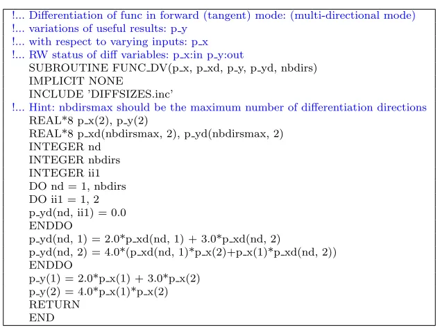
Table 5.1 A simple source program. . . 85
Table 5.2 A simple differential source program. . . 86
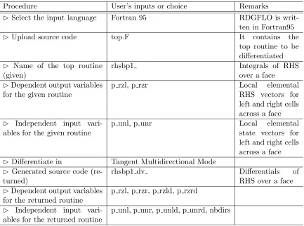
Table 5.3 Example: implementation of TAPENADE on RDGFLO. . . 87
Table 5.4 Pseudo code: contribution of face integrals for the block diagonal matrix D, lower matrixL, and upper matrixU. . . 88
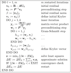
Table 5.5 Flowchart of the GMRES algorithm. . . 90
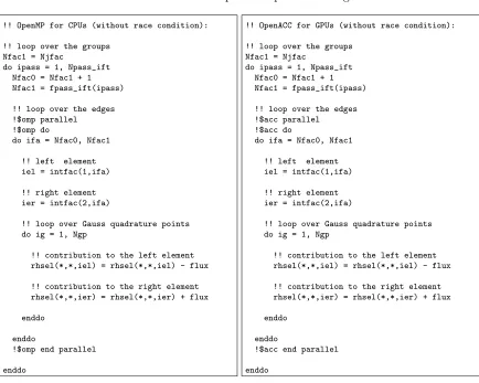
Table 6.1 An example of loop over the elements. . . 92
Table 6.2 An example of loop over the edges. . . 96
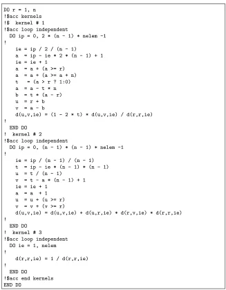
Table 6.3 Gauss-Jordan elimination without pivoting for ann×nmatrix. . . 98
Table 6.4 ACC version of GJE without pivoting forN elem matrices of sizen×n . . 99
Table 6.5 Workflow for the main loop over the explicit time iterations. . . 102
Table 6.6 Workflow for the data exchange and synchronization procedure. . . 103
Table 7.1 Part of the Nvidia GPGPU resource on the NCSU’s ARC cluster (donated by NVIDIA). . . 107
Table 7.2 Discretization errors and convergence rates obtained on the three succes-sively refined tetrahedral grids for inviscid subsonic flow past a sphere at a free-stream Mach number ofM∞= 0.5. . . 110
Table 7.3 Timing measurements of using TVDRK3+rDG(P1P2) methods for sub-sonic flow past a sphere. . . 114
Table 7.4 Timing measurements of weak scaling obtained on a cluster of NVIDIA Telsa C2050 GPU cards for using rDG methods with TVDRK3 for subsonic flow past a sphere. . . 115
Table 7.5 Timing measurements of usingp-multigrid DG/rDG methods for subsonic flow past a sphere. . . 115
Table 7.6 Timing measurements of using BDF1+DG/rDG methods for subsonic flow past a sphere. . . 117
Table 7.7 Timing measurements of weak scaling obtained on a cluster of NVIDIA Telsa C2050 GPU cards for using rDG methods with BDF1 for subsonic flow past a sphere. . . 118
Table 7.9 Timing measurements of weak scaling obtained on a cluster of NVIDIA Telsa C2050 GPU cards for using rDG methods with TVDRK3 for
tran-sonic flow over a Boeing 747 aircraft. . . 121
Table 7.10 Timing measurements of usingp-multigrid DG methods for transonic flow past a Boeing 747 aircraft. . . 122
Table 7.11 Timing measurements of using BDF1+DG/rDG methods for transonic flow past a Boeing 747 aircraft. . . 123
Table 7.12 Timing measurements of weak scaling obtained on a cluster of NVIDIA Telsa C2050 GPU cards for using rDG methods with BDF1 for transonic flow over a Boeing 747 aircraft. . . 124
Table 7.13 Timing measurements of using TVDRK3+rDG(P1P2) methods for laminar flow past a sphere. . . 128
Table 7.14 Timing measurements of weak scaling obtained on a cluster of NVIDIA Telsa C2050 GPU cards for using rDG methods with TVDRK3 for laminar flow past a sphere. . . 128
Table 7.15 Timing measurements of using TVDRK3+rDG(P1P2) methods for quasi-2D lid driven square cavity problem at Re = 10,000. . . 132
Table 7.16 Timing measurements of weak scaling obtained on a cluster of Nvidia Tesla C2050 GPU cards for a quasi-2D lid driven square cavity. . . 135
Table 7.17 Timing measurements of using RK4+rDG(P1P2) methods for Taylor-Green vortex problem . . . 140
Table 7.18 Timing measurements of weak scaling obtained on a cluster of Nvidia Tesla C2050 GPU cards for a Taylor-Green vortex problem. . . 140
Table 7.19 Order of accuracy on different type of grids for the steady nonlinear diffu-sion case. . . 159
Table 7.20 Order of accuracy for the 1D boundary layer case with different Re. . . 161
Table 7.21 Order of accuracy for the 2D steady advection-diffusion case on regular grids with differentν. . . 165
Table 7.22 Order of accuracy for the 2D steady advection-diffusion case on irregular grids with differentν. . . 166
Table 7.23 Order of accuracy for 2D steady advection-diffusion case on heterogeneous grids with differentν. . . 166
Table 7.24 Timing measurements of using hyperbolic DG/rDG methods for the quasi-2D steady advection-diffusion case on regular grids. . . 171
Table 7.25 Timing measurements of using hyperbolic DG/rDG methods for the quasi-2D steady advection-diffusion case on irregular grids. . . 171
Table 7.26 Timing measurements of using hyperbolic DG/rDG methods for the quasi-2D steady advection-diffusion case on heterogeneous grids. . . 172
Table 7.27 Order of accuracy for the 2D unsteady advection-diffusion case. . . 176
Table B.1 Abbreviation and description for various types of elements. . . 197
Table B.2 Shape functions for the 3-node triangle and their derivatives. . . 199
Table B.3 Shape functions for the 6-node triangle and their derivatives. . . 200
Table B.4 Shape functions for the 4-node quadrilateral and their derivatives. . . 202
Table B.6 Shape functions for the 4-node tetrahedron and their derivatives. . . 204
Table B.7 Shape functions for the 10-node tetrahedron and their derivatives. . . 206
Table B.8 Shape functions for the 8-node hexahedron and their derivatives. . . 207
Table B.9 Shape functions for the 6-node prism and their derivatives. . . 211
Table B.10 Shape functions for the 15-node prism and their derivatives. . . 213
Table B.11 Shape functions for the 5-node pyramid and their derivatives. . . 214
Table B.12 Shape functions for the 13-node pyramid. . . 216
Table C.1 Integration constants of Gaussian quadrature rules for a triangle. . . 218
Table C.2 Integration constants of Gaussian quadrature rules for a quadrilateral. . . . 219
Table C.3 Integration constants of Gaussian quadrature rules for a tetrahedron. . . . 220
Table C.4 Integration constants of Gaussian quadrature rules for a hexahedron. . . . 221
Table C.5 Integration constants of Gaussian quadrature rules for a prism. . . 222
LIST OF FIGURES
Figure 3.1 Representation of polynomial solutions using finite element shape func-tions: (a) Q1/P1; (b) Q2/P2. . . 23
Figure 3.2 Representation of polynomial solutions using a Taylor series expansion. . 25 Figure 3.3 Representation of the four face-neighboring cells surrounding a
tetrahe-dron (a) and the six face-neighboring cells surrounding a hexahetetrahe-dron (b). 32 Figure 3.4 Transformation of an element in (x, y) physical space into a canonical
element reference (ξ, η) space. . . 44 Figure 6.1 Domain decomposition by METIS for a tetrahedral grid (only surface
shown) for flow past a Boeing 747 aircraft, 16 partitions. . . 104 Figure 7.1 The NVIDIA Tesla GPGPUs used in the present work:(a) C2050 (448
stream processors, 3GB memory); (b) K20c (2496 stream processors, 5GB memory). . . 107 Figure 7.2 A sequence of three successively globally refined tetrahedral grids for
in-viscid subsonic flow past a sphere. . . 110 Figure 7.3 Computed density contours in the flow field by the DG(P1) (a–c) and
rDG(P1P2) (d–f) on the tetrahedral grids for inviscid subsonic flow past
a sphere at M∞= 0.5. . . 111 Figure 7.4 Computed pressure contours in the flow field by the DG(P1) (a–c) and
rDG(P1P2) (d–f) on the tetrahedral grids for inviscid subsonic flow past
a sphere at M∞= 0.5. . . 112 Figure 7.5 Computed Mach number contours in the flow field by the DG(P1) (a–c)
and rDG(P1) (d–f) on the tetrahedral grids for inviscid subsonic flow past
a sphere at M∞= 0.5. . . 113 Figure 7.6 Plot of the timing measurements for inviscid subsonic flow past a sphere
with a fixed problem size (approximately half million elements) per GPU card (NVIDIA Tesla C2050) using TVDRK3+DG/rDG scheme: (a) Unit running time versus the number of GPU cards; (b) Parallel efficiency versus the number of GPU cards. . . 116 Figure 7.7 Subsonic flow past a sphere at a free-stream Mach number of M∞= 0.5:
(a) Comparison of convergence history versus CPU time between TV-DRK3 and p-multigrid methods for DG(P1); (b) Comparison of
conver-gence history versus CPU time between TVDRK andp-multigrid methods for rDG(P1P2). . . 116
Figure 7.8 Averaged one main time loop run times (in seconds) for running implicit rDG(P1P2) on the finest mesh for the inviscid sphere case. . . 117
Figure 7.10 Inviscid transonic flow over a Boeing 747 aircraft computed using rDG(P1P2),
(a) the tetrahedral grid used for computation (N elem= 253,577,N poin= 48,851,N bf ac= 23,616, ) (b) computed density contours, (c) computed Mach number contours, and (d) computed pressure contours. . . 120 Figure 7.11 Plot of the timing measurements for inviscid transonic flow over a Boeing
747 aircraft with a fixed problem size (approximately half million ele-ments) per GPU card (NVIDIA Tesla C2050) using TVDRK3+DG/rDG scheme: (a) Unit running time versus the number of GPU cards; (b) Par-allel efficiency versus the number of GPU cards. . . 122 Figure 7.12 Transonic flow past a Boeing 747 aircraft at a free-stream Mach
num-ber of M∞ = 0.85 and a angle of attack of α = 2◦: (a) Comparison of convergence history versus CPU time between TVDRK and p-multigrid methods for DG(P1); (b) Comparison of convergence history versus CPU
time between TVDRK and p-multigrid methods for rDG(P1P2). . . 123
Figure 7.13 Plot of the timing measurements for transonic flow over a Boeing 747 aircraft with a fixed problem size (approximately half million elements) per GPU card (NVIDIA Tesla C2050) using BDF1+DG/rDG scheme: (a) Unit running time versus the number of GPU cards; (b) Parallel efficiency versus the number of GPU cards. . . 125 Figure 7.14 (a) Plot of the surface meshes of the tetrahedral gridfor laminar flow past
a sphere at M∞ = 0.5 and Re = 118; (b) plot of the computed velocity streamtraces on the symmetry plane using rDG(P1P2). . . 126
Figure 7.15 Plot of the computed contours obtained by rDG(P1P2) on the surface
meshes in the flow field atM∞= 0.5 and Re = 118: (a) pressure contours; (b) Mach number contours. . . 127 Figure 7.16 Plot of the timing measurements for laminar flow past a sphere with a
fixed problem size (approximately half million elements) per GPU card (NVIDIA Tesla C2050) using TVDRK3+DG/rDG scheme: (a) Unit run-ning time versus the number of GPU cards; (b) Parallel efficiency versus the number of GPU cards. . . 129 Figure 7.17 A quasi-2D lid driven square cavity flow at a lid velocity ofvB= (0.2,0,0)
and a series of Reynolds number: (a) The sparse hexahedral grid (32×32× 2 grid points) used in the verification test, (b) Re = 100, (c) Re = 1000, and (d) Re = 10,000. . . 131 Figure 7.18 Profiles of the normalized velocity componentsu/uBandv/uBon a sparse
hexahedral grid (32×32×2 grid points) for a quasi-2D lid driven square cavity at a lid velocity of vB = (0.2,0,0), and a Reynolds number of Re = 100. . . 132 Figure 7.19 Profiles of the normalized velocity componentsu/uBandv/uBon a sparse
Figure 7.20 Profiles of the normalized velocity componentsu/uBandv/uBon a sparse hexahedral grid (32×32×2 grid points) for a quasi-2D lid driven square cavity at a lid velocity of vB = (0.2,0,0), and a Reynolds number of Re = 10,000. . . 134 Figure 7.21 Plot of the timing measurements for a quasi-2D lid driven square cavity
with a fixed problem size (approximately half million elements) per GPU card (Nvidia Tesla C2050): (a) Unit running time versus the number of GPU cards, (b) Parallel efficiency versus the number of GPU cards . . . . 136 Figure 7.22 The isosurfaces of Q2 criterion colored by velocity magnitude at time
t= 8tc. . . . 139 Figure 7.23 Evolution of the dimensionless kinetic energy as a function of the
dimen-sionless time using RK4. . . 140 Figure 7.24 Evolution of the dimensionless kinetic energy dissipation rate as a function
of the dimensionless time using RK4. . . 141 Figure 7.25 Evolution of the dimensionless enstrophy rate as a function of the
dimen-sionless time using RK4. . . 141 Figure 7.26 Plot of the timing measurements for a 3D Taylor-Green Vortex with a
fixed problem size (approximately half million elements) per GPU card (Nvidia Tesla C2050): (a) Unit running time versus the number of GPU cards. (b) Parallel efficiency versus the number of GPU cards. . . 142 Figure 7.27 The second mesh of every type, that is, 17×17 regular grid, 17×17
irregular grid, and 23×21 heterogeneous grid. . . 143 Figure 7.28 Distribution ofR in the coarsest irregular mesh (left) and heterogeneous
mesh (right). . . 144 Figure 7.29 Grid refinement study of the hyperbolic rDG methods for the steady
scalar diffusion case without source term on regular grids using implicit BDF1 . . . 146 Figure 7.30 Grid refinement study of the hyperbolic rDG methods for the steady
scalar diffusion case without source term on regular grids using implicit BDF1. . . 147 Figure 7.31 Grid refinement study of the hyperbolic rDG methods for the steady scalar
diffusion case without source term on heterogeneous grids using implicit BDF1. . . 147 Figure 7.32 Comparison between hyperbolic rDG methods and BR2 scheme in terms
of order of accuracy for the steady scalar diffusion case without source term on regular grids using explicit TVDRK3. . . 148 Figure 7.33 Comparison between hyperbolic rDG methods and BR2 scheme in terms
of order of accuracy for the steady scalar diffusion case without source term on irregular grids using explicit TVDRK3. . . 148 Figure 7.34 Comparison between hyperbolic rDG methods and BR2 scheme in terms
Figure 7.35 Comparison between hyperbolic rDG methods and BR2 scheme in terms of CPU time for the steady scalar diffusion case without source term on
17×17 regular grids using explicit TVDRK3. . . 149
Figure 7.36 Comparison between hyperbolic rDG methods and BR2 scheme in terms of CPU time for the steady scalar diffusion case without source term on 17×17 irregular grids using explicit TVDRK3. . . 150
Figure 7.37 Comparison between hyperbolic rDG methods and BR2 scheme in terms of CPU time for the steady scalar diffusion case without source term on 23×21 heterogeneous grids using explicit TVDRK3. . . 150
Figure 7.38 Time steps and CPU time required to reach the steady state for regular grids using explicit TVDRK3. . . 151
Figure 7.39 Grid refinement study of the steady scalar diffusion case with source term on regular grids using implicit BDF1. . . 152
Figure 7.40 Grid refinement study of the steady scalar diffusion case with source term on irregular grids using implicit BDF1. . . 153
Figure 7.41 Grid refinement study of the steady scalar diffusion case with source term on heterogeneous grids using implicit BDF1. . . 153
Figure 7.42 Grid refinement study of the steady tensor diffusion case with source term on regular grids using implicit BDF1. . . 155
Figure 7.43 Grid refinement study of the steady tensor diffusion case with source term on irregular grids using implicit BDF1. . . 155
Figure 7.44 Grid refinement study of the steady tensor diffusion case with source term on heterogeneous grids using implicit BDF1. . . 156
Figure 7.45 Grid refinement study of the steady nonlinear diffusion case on regular grids using implicit BDF1. . . 157
Figure 7.46 Grid refinement study of the steady nonlinear diffusion case on irregular grids using implicit BDF1. . . 158
Figure 7.47 Grid refinement study of the steady nonlinear diffusion case on heteroge-neous grids using implicit BDF1. . . 159
Figure 7.48 Grid refinement study for the 1D boundary layer case, Re= 10−8. . . 162
Figure 7.49 Grid refinement study for the 1D boundary layer case, Re= 1. . . 162
Figure 7.50 Grid refinement study for the 1D boundary layer case, Re= 108. . . 163
Figure 7.51 Grid refinement study for the 2D steady advection-diffusion case on reg-ular grids with ν= 10−8,Re =√5×10⁸. . . 167
Figure 7.52 Grid refinement study for the 2D steady advection-diffusion case on reg-ular grids with ν= 1,Re =√5. . . 167
Figure 7.53 Grid refinement study for the 2D steady advection-diffusion case on reg-ular grids with ν= 108,Re =√5×10⁻⁸. . . 168
Figure 7.54 Grid refinement study for the 2D steady advection-diffusion case on ir-regular grids with ν = 10−8,Re =√5×10⁸. . . 168
Figure 7.55 Grid refinement study for the 2D steady advection-diffusion case on ir-regular grids with ν = 1,Re =√5. . . 169
Figure 7.57 Grid refinement study for the 2D steady advection-diffusion case on
het-erogeneous grids with ν= 10−8,Re =√5×10⁸. . . 170
Figure 7.58 Grid refinement study for the 2D steady advection-diffusion case on het-erogeneous grids with ν= 1,Re =√5. . . 170
Figure 7.59 Grid refinement study for the 2D steady advection-diffusion case on het-erogeneous grids with ν= 108,Re =√5×10⁻⁸. . . 171
Figure 7.60 Grid refinement study on regular grids for the 1D unsteady advection-diffusion case. . . 174
Figure 7.61 Comparison between the numerical solutions obtained by the hyperbolic rDG methods and DDG methods for the 1D unsteady advection-diffusion case, tend= 10−3 (5 periods). . . 174
Figure 7.62 Grid refinement study on regular grids for 2D unsteady advection-diffusion case. . . 175
Figure 7.63 Grid refinement study on irregular grids for 2D unsteady advection-diffusion case. . . 176
Figure B.1 Representation of the 3-node triangular element. . . 197
Figure B.2 Representation of barycentric coordinates for a triangle in physical space. 198 Figure B.3 Representation of barycentric coordinates for a reference triangle. . . 198
Figure B.4 Representation of the 6-node triangular element. . . 199
Figure B.5 Representation of the 4-node quadrilateral element. . . 201
Figure B.6 Representation of the 8-node quadrilateral element. . . 202
Figure B.7 Representation of the 4-node tetrahedral element. . . 203
Figure B.8 Representation of barycentric coordinates for a tetrahedron in physical space. . . 204
Figure B.9 Representation of the 10-node tetrahedral element. . . 205
Figure B.10 Representation of the 8-node hexahedral element. . . 207
Figure B.11 Representation of the 20-node hexahedral element. . . 208
Figure B.12 Representation of the 6-node prismatic element. . . 211
Figure B.13 Representation of the 15-node prismatic element. . . 212
Figure B.14 Representation of the 5-node pyramidal element. . . 214
Chapter
1
Introduction
1.1
General-Purpose Graphics Processing Unit for
Computa-tional Fluid Dynamics
Nowadays, with increasing attention in science and engineering field, the General-Purpose Graphics Processing Unit (GPGPU [123]) technology, which is essentially a shared memory vector device, offers a new opportunity to dramatically accelerate the CPU-based code by of-floading compute-intensive portions of the application to the GPU, while the remainder of the computer program still suns on the CPU, which also make it expected to be a major compute unit in the near future. From a user’s perspective, the solvers simply run much faster.
Computational Fluid Dynamics (CFD), a branch of mechanics that applies numerical way to solve fluid dynamics problem, has been one of the most significant applications on su-percomputers. The presence of GPGPU could outperform the traditional CPU based par-allel computing and therefore to meet the needs to solving complex simulation CFD prob-lem [7, 21, 22, 30, 32, 33, 50, 60, 61, 106, 127, 140].
FD method solver for large calculation on multiblock structured grids, Kl¨ockner et al. [67] developed a 3D unstructured high-order nodal DG method solver for the Maxwell’s equations, Corrigan et al. [34] proposed a 3D FV solver for compressible inviscid flow on unstructured tetrahedral grids and Zimmerman et al. [162] presented a SD method solver for the Navier-Stokes equations on unstructured hexahedral grids. Nevertheless, the development of CUDA capabilities extended from an existing CFD solver is not a trivial job, because people have to define an explicit layout of the threads on the GPU (numbers of blocks and numbers of threads) for each kernel function [63]. Such a project often requires tremendous hours in programming, as developers have to rewrite all the core content of the source code. Moreover, for a production-level solver, people also need to address both the short-term and long-term investment concerns like the cost and profit, as well as platform portability. These factors can often set people back from investing on GPU computing for their well-established solution products. Even a research-oriented CFD solver is concerned, people may be more inclined to maintain compatibility of their codes across multiple platforms, instead of pursuing performance on one particular platform at the price of being unable to run their codes on other mainstream platforms. Therefore, the development strategy of a CFD solver based on one unique model like CUDA might be a risky long-term investment with unclear prospect of the vendor’s own plan. Fortunately, NVIDIA CUDA is not the sole player in this area. Two other programming models on GPU include OpenCL [139], the currently dominant open GPGPU programming model (but dropped from further discussion because it does not support the FORTRAN programming language) and OpenACC [149], a new programming standard for parallel computing developed by Cray, CAPS, NVIDIA and PGI.
is available in the commercial compilers from PGI, Cray, and CAPS. OpenUH is an Open64-based open source OpenACC compiler, developed by HPCTools group from the University of Houston. In addition, the GCC (GNU Compiler Collection) project team is also working toward supporting OpenACC in the GCC compilers.
A typical GPU has hundreds or even thousands of computation cores. However, compared with a typical CPU core, those on GPU card would has much less computation power and local cache memory. Therefore, for optimal performance on GPU, the algorithm should be divided into smaller units, thus occupying more cores with the same amount of work. In addition, the amount of data each core processes should be kept as small as possible. The latter aspect is particularly important for solving a block-sparse system, which consists of a large amount of square sub-matrices of an identical size. On each sub-matrix, if the operation is mapped to one GPU core, the algorithm easily becomes heavily memory-bounded, especially when the dimension of the sub-matrix is large, resulting in serious performance penalty. In other words, the key to achieve higher speed up factor on GPU platform is fine granularity.
Nevertheless, it is generally difficult to port the implicit algorithm to GPU platform. First of all, the size of sub-matrices would cause the memory-bounded issue, especially for higher order method. Secondly, it is not straightforward to utilize some popular liner solver or preconditioner like Symmetric Gauss-Seidel (SGS) or Lower Upper-Symmetric Gauss-Seidel (LU-SGS) due to the inherent data dependency. Additionally, the iterative solver like Generalized Minimal Residual (GMRES) method would require additional storage for some auxiliary arrays, which would bring challenge to GPU computing since the local cache memory of GPGPU is limited.
1.2
Reconstructed Discontinuous Galerkin Methods
and finite volume (FV) methods. As in classical finite element methods, accuracy is obtained by means of high-order polynomial approximation within an element rather than by wide stencils as in the case of finite volume methods. The physics of wave propagation is, however, accounted for by solving the Riemann problems [141] that arise from the discontinuous representation of the solution at element interfaces. In this respect, the methods are therefore similar to finite volume methods. A more comprehensive overview of the discontinuous Galerkin methods is given by Cockburn et al.[27].
The discontinuous Galerkin methods are attractive to many researchers due to the fact that they have many promising features. First of all, the DG methods have several useful mathematical properties with respect to conservation, stability and convergence. Also, they can be easily extended to higher-order (>2nd) approximation. Additionally, the DG methods are well suited for complex geometries since they can be applied on unstructured grids. In addition, the methods can also handle non-conforming elements, where the grids are allowed to have hanging nodes. As for parallelization, since DG methods are compact and each element is independent, they are highly parallelizable [69, 92]. Since the elements are discontinuous, and the inter-element communications are minimal, domain decomposition can be effectively employed. The compactness also allows for structured and simplified coding for the methods. Meanwhile, since refining or coarsening a grid can be achieved without considering the continuity restriction commonly associated with the conforming elements, they allow easy implementation of hp-refinement [18, 55, 108, 121, 148], for example, the order of accuracy, or shape, can vary from element to element. Last but not least, the DG methods have the ability to compute low Mach number flow problems [10, 86] without recourse to the time-preconditioning techniques normally required for the finite volume methods.
In spite of the enormous advances in the theoretical and numerical analysis of the DG methods [4, 5, 6, 11, 12, 13, 15, 26, 28, 29, 31, 55, 56, 56, 65, 66, 68, 95, 121, 124, 126, 129, 130, 131, 143, 144], the DG methods have a number of weaknesses that have yet to be addressed, before they can be robustly used for flow problems of practical interest in complex configuration environment. In particular, how to effectively control spurious oscillations in the presence of strong discontinuities, how to reduce the computing costs, and how to efficiently solve elliptic problems or discretize diffusion terms in the parabolic equations remain three most challenging and unresolved issues for the DG methods.
adds explicitly consistent artificial viscosity terms to the discontinuous Galerkin discretization. The main disadvantage of this method is that it usually requires some user-specified parameters, which can be both grid and problem dependent. As for the slope limiting, the classical techniques are not directly applicable for high-order DG methods because of the presence of volume integral terms in the formulation. Therefore, the slope limiter is not integrated in the computation of the residual, but effectively acts as a post-processing filter. Many slope limiters used in the finite volume methods can then be used or modified to meet the needs of the DG methods. Unfortunately, the use of the limiters will reduce the order of accuracy to first order in the presence of discontinuities. Furthermore, the active limiters in the smooth extrema will pollute the solution in the flow field and ultimately destroy the higher-oder accuracy of the DG methods. Indeed, it is not an exaggeration to state that the design of efficient, effective, and robust limiters is one of the bottlenecks in the development of the DG methods for solving the conservation laws. Most efforts in the development of the DG methods have primarily been focused on the exploration of their advantages such as higher-order spatial discretization, posteriori error estimation, adaptive algorithms, and parallelization.
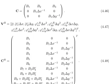
requirements can still be extremely demanding. The block diagonal matrix requires a storage of (N degr×N etot)×(N degr×N etot)×N elem, whereN degris the number of degree of freedom for the polynomial (3 for P1, 6 for P2, and 10 for P3 for triangular element in 2D; 4 for P1,
10 for P2, and 20 for P3 for tetrahedral element in 3D), N etot is the number of components
in the solution vector (4 for 2D, and 5 for the three-dimensional Navier-Stokes equations), and
N elemis the number of elements for the grid. For example, for a 4th-order (cubic polynomial finite element approximation P3) DG method in 3D, the storage of this block diagonal matrix
alone requires 10,000 words per element.
In order to reduce the high computing costs associated with the DG methods, Dumbser et al.[39,41,42] have introduced a new family of reconstructed DG methods, termed PnPmschemes and referred to as rDG(PnPm) in this work, where Pm indicates that a piecewise polynomial of degree of n is used to compute the fluxes and source term. The rDG(PnPm) schemes are designed to enhance the accuracy of the discontinuous Galerkin method by increasing the order of the underlying polynomial solution. The beauty of the rDG(PnPm) schemes is that they provide a unified formulation for both the finite volume and DG methods, and contain both the classical finite volume and standard DG methods as two special cases of the rDG(PnPm) schemes, and thus allow for a direct efficiency comparison. Whenn= 0, i.e., a piecewise constant polynomial is used to represent a numerical solution, the rDG(P0Pm) scheme is nothing but
the classical high-order finite volume scheme, where a polynomial solution of degreem(m≥1) is reconstructed from a piecewise constant solution. When m =n, the reconstruction reduces to the identity operator, and the rDG(PnPn) scheme yields a standard DG method.
Traditionally, DG methods would either use the standard Lagrange or hierarchical node-based finite element basis functions to represent numerical polynomial solutions in each element. As a result, the unknowns to be solved are the variables at the nodes and the polynomial solutions are dependent on the shape of elements. In the present work, the numerical polynomial solutions are represented using a Taylor series expansion at the centroid of the cell, which can be further expressed as a combination of cell-averaged variables and their derivatives at the centroid of the cell. The unknowns to be solved in this formulation are cell-averaged values and their derivatives at the center of the cells, regardless of the element shapes. In other words, by using this formulation, the DG method can be easily implemented on arbitrary grids. Therefore, The numerical method based on this formulation has the ability to compute the 1D, 2D, and 3D problems using the very same code, which greatly alleviates the need and pain for code maintenance and upgrade. Also, due to the fact that the basis functions are hierarchic, the implementation ofp-multigrid andp-refinement methods has become straightforward.
the success of the rDG(PnPm) schemes. In Dumbser’s work, a higher-order polynomial solution is reconstructed using an L2 projection, requiring it indistinguishable from the underlying DG solutions in the contributing cells in the weak sense. The resulting over-determined system is then solved by using a least-squares method that guarantees exact conservation, not only of the cell averages but also of all higher-order moments in the reconstructed cell itself, such as slopes and curvatures. However, this conservative least-squares reconstruction approach is computa-tionally expensive, as the L2 projection, i.e., the operation of integration, is required to obtain the resulting over-determined system. Furthermore, the reconstruction might be problematic for a boundary cell, where the number of the adjacent face-neighboring cells might not be enough to provide the necessary information to recover a polynomial solution of a desired order. Fortu-nately, the projection-based reconstruction is not the only way to obtain a polynomial solution of higher order from the underlying discontinuous Galerkin solutions. In the reconstructed DG method using a Taylor basis [92, 93, 94, 97, 99] developed by Luo et al. for the solution of the compressible Euler/Navier-Stokes equations on arbitrary grids, a higher-order polynomial so-lution is reconstructed by using a strong interpolation, requiring point values and derivatives to be interpolated on the adjacent face-neighboring cells. The resulting over-determined linear system of equations is then solved in the least-squares sense. This reconstruction scheme only involves the von Neumann neighborhood, and thus is compact, simple, robust, and flexible. Like the projection-based reconstruction, the strong reconstruction scheme guarantees exact conservation, not only of the cell averages but also of their slopes due to a judicious choice of the Taylor basis. More recently, Zhang et al. [160, 161] presented a class of hybrid DG/FV methods for the conservation laws, where the second derivatives in a cell are obtained from the first derivatives in the cell itself and its neighboring cells using a Green-Gauss reconstruction widely used in the finite volume methods. This also provides a fast, simple, and robust way to obtain higher-order polynomial solutions. More recently, Luo et al.[98, 100] have conducted a comparative study for these three reconstructed discontinuous Galerkin methods rDG(P1P2)
for solving the 2D Euler equations on arbitrary grids. It is found that all the three reconstructed discontinuous Galerkin methods can deliver the desired third-order accuracy and significantly improve the accuracy of the underlying second-order DG method, although the least-squares reconstruction method provides the best performance in terms of both accuracy and robustness. However, the attempt to directly extend the least-squares rDG method to solve the 3D Euler equations on tetrahedral grids is not successful. Like the second-order cell-centered finite volume methods, i.e., rDG(P0P1), the resultant rDG(P1P2) method is numerically unstable.
Although the rDG(P0P1) methods are in general stable in 2D and on Cartesian or structured
when the reconstruction stencils only involve von Neumann neighborhood, i.e., adjacent face-neighboring cells [51]. Unfortunately, the least-squares rDG(P1P2) method exhibits the same
linear instability, which can be overcome by using extended reconstruction stencils. However, this is achieved at the expense of sacrificing the compactness of the underlying DG methods. Furthermore, these linear reconstruction-based DG methods will suffer from the non-physical oscillations in the vicinity of strong iscontinuities for the compressible Euler equations. Alterna-tively, the essentially non-oscillatory (ENO), weighted essentially non-oscillatory (WENO) and Hermite-WENO schemes can be used to reconstruct a higher-order polynomial solution, which can not only enhance the order of accuracy of the underlying DG method but also achieve both the linear and non-linear stability.
The ENO schemes were initially introduced by Harten et al. [54], in which oscillations up to the order of the truncation error are allowed to overcome the drawbacks and limitations of limiter-based schemes. ENO schemes avoid interpolation across high-gradient regions through biasing of the reconstruction. This biasing is achieved by reconstructing the solution on several stencils at each location and selecting the reconstruction which is in some sense the smoothest. This allows ENO schemes to retain higher-order accuracy near high-gradient regions. However, the selection process can lead to convergence problems and loss of accuracy in regions with smooth solution variations. To counter these problems, the so-called weighted ENO (WENO) scheme introduced by Liu et al [75] is designed to present better convergence rate for steady-state problems, better smoothing for the flux vectors, and better accuracy using the same stencils than the ENO scheme. The WENO scheme uses a suitably weighted combination of all reconstructions rather than just the one that is judged to be the smoothest. The weighting is designed to favor the smooth reconstruction in the sense that its weight is small if the oscillation of a reconstructed polynomial is high, and its weight is order of one if a reconstructed polynomial has low oscillation. Qiu and Shu initiated the use of the WENO scheme as limiters for the DG method [131] for solving the 1D and 2D Euler equations on structured grids. Later on, they constructed a class of WENO schemes based on Hermite polynomials, termed as Hermite WENO schemes and applied these schemes as limiters for the DG methods [129,130]. The main difference between Hermite-WENO and WENO schemes is that the former has a more compact stencil than the latter for the same order of accuracy.
was also presented by Friedrich [46] and Hu et al. [59].
The Hermite-WENO schemes has been developed on 1D and 2D structured grids for the DG methods by Balsara et al [8], where the Hermite-WENO reconstruction scheme is relatively simple and straightforward. In the work presented, a Taylor basis [97]reconstruction-based DG method, rDG(P1P2), based on a Hierarchical WENO reconstruction scheme, termed as
HWENO(P1P2) [99], is developed for the solution of the compressible Euler and Navier-Stokes
equations on single-type and hybrid unstructured grids in 3D [150]. This reconstructed DG method is designed not only to reduce the high computing costs of the DG methods, but also to avoid spurious oscillations in the vicinity of strong discontinuities, thus effectively overcoming two of the three most severe shortcomings of the DG methods and ensuring the linear and non-linear stability of the reconstructed DG method. In this rDG(P1P2) method, a quadratic
solution is obtained through the HWENO(P1P2) reconstruction in three steps: (1) all the
sec-ond derivatives (P2) in each cell are first reconstructed using the solution variables (P0) and
their first derivatives (P1) from adjacent face-neighboring cells via a least-squares method; (2)
a WENO reconstruction would be performed to obtain the final second derivatives in each cell based on the reconstructed second derivatives in the cell itself and its adjacent face-neighboring cells; (3) the gradients of the quadratic polynomial solutions are then modified using a WENO reconstruction. As one can see, the linear stability of the rDG method is ensured through step 2 while the non-physical oscillations in the vicinity of strong discontinuities is eliminated in step 3 and thus to ensure the non-linear stability of the developed scheme. This reconstruction scheme, by taking advantage of handily available and yet valuable information, namely the gradients in the context of the DG methods, only involves von Neumann neighborhood and thus is compact, simple, robust and flexible.
rDG(PnPm) stands for the reconstruction DG method based on least squares method.
As the underlying DG(P1) method is second order, and the basis functions are at most
linear functions, fewer integration points are then required for both volume and face integrals, and the number of unknowns (the number of degrees of freedom) remains the same as for the DG(P1) method. Consequently, this rDG(P1P2) method is more efficient than its third-order
DG(P2) counterpart.
The DG methods are indeed a natural choice for the solution of the hyperbolic equations, such as the compressible Euler equations. However, the DG formulation is far less certain and advantageous for elliptic problems or parabolic equations such as the compressible Navier-Stokes equations, where diffusive fluxes exist and which require the evaluation of the solution derivatives at the interfaces. Taking a simple arithmetic mean of the solution derivatives from the left and right is inconsistent, because it does not take into account a possible jump of the solutions. A number of numerical methods have been proposed in the literature to address this issue, such as those by Bassi and Rebay [11, 14, 15], Cockburn and Shu [29], Baumann and Oden [18], Peraire and Persson [124], and many others. Arnoldet al. [6] have analyzed a large class of DGM for second-order elliptic problems in a unified formulation. All these methods have introduced in some way the influence of the discontinuities in order to define correct and consistent diffusive fluxes. Gassner et al. [47] introduced a numerical scheme based on the exact solution of the diffusive generalized Riemann problem for the DGM. Liu et al. [73, 74] proposed a direct discontinuous Galerkin (DDG) method to solve diffusion problems based on the direct weak formulation for solutions of parabolic equations. Cheng et al. [25] successfully extended the DDG method to solve the compressible Navier-Stokes equations on arbitrary grids. Luo et al. have developed a reconstructed discontinuous Galerkin method using an inter-cell reconstruction [94] for the solution of the compressible Navier-Stokes equations. Unfortunately, all these methods seem to require substantially more computational effort than the classical continuous finite element methods, which are naturally more suited for the discretization of elliptic problems. There is also an approach where a scalar diffusion scheme is derived from a hyperbolic diffusion formulation [112, 113]. It has been extended to higher-order in the context of the residual-distribution method [3], but has not been extended in the DG methods beyond second-order.
feature of the FOHS method from other FOS methods, by adding pseudo time derivatives to the first-order system. It thus generates a system of pseudo-time evolution equations for the solution and the derivatives in the partial differential equation (PDE) level, not in the dis-cretization level as in DG methods. The hyperbolic reformulation in the PDE level would allow a dramatic simplification in the discretization as the well-established methods can be directly applied to the viscous terms. The FOHS method is especially attractive in the context of the DG methods since it allows the use of inviscid algorithms for the viscous terms and thus greatly simplifies the discretization of the compressible Navier-Stokes equations. Moreover, the FOHS method yields a numerical scheme that can achieve the same order of accuracy in the solution and its derivatives on irregular grids and high-quality noise-free gradients on such grids. This is a very important feature for unstructured-grid viscous simulations, in which target quantities are derivatives, e.g., viscous stresses and heat fluxes.
A challenge in combining the DG method and the FOHS method lies in a very large num-ber of discrete unknowns arising from both methods. For a scalar equation in two dimensions, the FOHS method introduces two derivatives as additional variables, and a P1 DG method
introduces three degrees of freedom (DoFs) for each variable (solution, and two derivatives), resulting in the total of nine degrees of freedom. In 2015, Nishikawa noticed that these degrees of freedom can be significantly reduced by unifying inter-related high-order moments of the derivative variables and extending the idea of Scheme-II [114] to replace high-order moments of a solution polynomial by the derivative variables. He has shown that the total number of degrees of freedom can be reduced from nine to six while the order of polynomial is upgraded to quadratic for the solution variable. The resulting approximation is comparable to a conventional P2 DG method. Therefore, if compared with a one-order higher conventional DG method, the
FOHS method requires virtually no increase in the degrees of freedom. The method extends systematically to arbitrary order of accuracy: Pk hyperbolic DG method gives comparable ac-curacy as Pk+1 DG method for the same number of degrees of freedom. Later, the method was
More importantly, the method does not contribute to reducing the cost of the DG method. In this study, we explore the combination of the FOHS method and the rDG method in order to reduce the cost of the DG method towards affordable high-order unstructured-grid methods for practical applications.
Another difficulty would arise when it comes to unsteady problems. Typically, implicit-time stepping schemes are employed in the hyperbolic method, and all previous developments rely on the backward difference formulas (BDF) [79,120]. The first- and second-order BDF formulas are unconditionally stable (L-stable), and thus suitable for practical applications. However, higher-order (≥3) backward-difference formulas are only conditionally stable. It is highly desirable to develop unconditionally-stable high-order hyperbolic schemes for unsteady problems. Also, the high-order BDF method is not self-starting, requiring several lower order BDF methods at the starting stages. Furthermore, the time step would need to be fixed unless some further modifica-tion is made, like the variable time step BDF methods [120]. To overcome these difficulties, we consider an explicit first stage, single diagonal coefficient, diagonally implicit Runge-Kutta time integration scheme (ESDIRK) [19] and demonstrate the unsteady capability of the developed hyperbolic schemes. Compared with BDF methods, implicit Runge-Kutta (IRK) methods are A-stable and L-stable for arbitrary order in time. Also, variable time step sizes can be easily applied. Moreover, ESDIRK schemes are self-starting, i.e., one does not need to set up different temporal schemes at the beginning. Although ESIRK schemes would be more computationally expensive than the BDF counterpart for the same time step size, the cost can be reduced by taking a larger time step without encountering instability and maintaining the design order of accuracy.
1.3
Motivation and Goals
The objective of the effort presented in this Ph.D. work is to develop and port a 3D legacy code, reconstructed discontinuous Galerkin Flow solver (RDGFLO) for the compressible Navier-Stokes equations, onto GPU platforms using OpenACC. This third-order accurate rDG method is based on a hierarchical weighed essentially non-oscillatory reconstruction scheme, termed as HWENO(P1P2) to indicate that a quadratic polynomial solution is obtained from the
underly-ing linear polynomial DG solution via a hierarchical WENO reconstruction. The HWENO(P1P2)
is designed not only to enhance the accuracy of the underlying DG(P1) method but also to
ensure non-linear stability of the rDG method. In this reconstruction scheme, a quadratic poly-nomial (P2) solution is first reconstructed using a least-squares approach from the underlying
a Hermite WENO reconstruction, which is necessary to ensure the linear stability of the rDG method on 3D unstructured grids. The first derivatives of the quadratic polynomial solution are then reconstructed using a WENO reconstruction in order to eliminate spurious oscillations in the vicinity of strong discontinuities, thus ensuring the non-linear stability of the rDG method. By taking advantages of the OpenACC parallel programing model, the presented scheme re-quires the minimum code intrusion and algorithm alteration to upgrade a legacy CFD solver without much extra time of effort in programming, resulting a unified portable code for both CPU and GPU platforms.
In this work, hyperbolic rDG methods based on first order hyperbolic system (FOHS) are developed. Both least squares reconstruction and variational reconstruction has been employed to obtain higher order numerical solutions while remaining the total degrees of freedom rel-atively small. By combining the advantages of the FOHS formulation and the rDG methods, an effort has been made to develop a more reliable, accurate, efficient, and robust method for solving some model equations including diffusion equation, advection-diffusion equation and ultimately the incompressible and compressible Navier-Stokes equations on fully irregular, adaptive, anisotropic, unstructured grids.
In this study, both underlying DG(P1) scheme and rDG(P1P2) scheme which indicates that
a quadratic polynomial solution is obtained from the underlying linear polynomial DG solution via a hierarchical WENO reconstruction, are ported onto GPGPU platform. Both multi-stage explicit Runge-Kutta and simple implicit backward Euler methods are implemented for time advancement. Additionally, for the unsteady case solved by the newly developed hyperbolic rDG scheme, implicit Runge-Kutta has also been employed. Meanwhile p-multigrid technics are also adopted in the study to accelerate the convergence. For p-multigrid scheme, DG(P1)
and rDG(P1P2) are implemented as higher level method while DG(P0) scheme are used as
meshes of approximately the same size.
A number of inviscid and viscous flow problems are presented to verify the implementation of the developed scheme. Strong scaling tests are carried out to compare the unit running time on single GPU and single CPU to obtain the speed up factor of the developed methods. Also, weak scaling tests are carried out for several cases to test the parallel efficiency for multi-GPU computing by comparing the unit running time with different number of multi-GPU cards for an approximately fixed problem size per GPU card. The results of timing measurements indicate that this OpenACC-based parallel scheme is able to significantly accelerate the solving procedure for the equivalent legacy CPU code. Numerical experiments of the model equations for the developed hyperbolic rDG methods demonstrate that the presented methods are able to achieve the designed optimal order of accuracy for both solutions and their derivatives on regular, irregular, and heterogeneous girds, and outperform the conventional diffusive DG method like BR2, DDG, in terms of the magnitude of the error, the order of accuracy, the size of time steps, and the CPU times required to achieve steady state solutions, indicating that the developed hyperbolic rDG methods provide an attractive and probably an even superior alternative to deal with the diffusive fluxes.
In summary, the developed GPU accelerated rDG method has a great potential to become a viable, attractive, competitive and ultimately superior DG method over the current state-of-the-art second-order finite volume methods.
Chapter
2
Governing Equations of Fluid Dynamics
In this chapter, the governing equations of the physical flow models used in this work are briefly described: the Navier-Stokes equations (§2.1) and the Euler equations (§2.2). The nondimen-sionalization of the governing equations are described in the last section.
2.1
Navier-Stokes Equations
The Navier-Stokes equations governing unsteady compressible viscous flows can be expressed as
∂U ∂t +
∂Fk(U)
∂xk
= ∂Gk(U)
∂xk
, (2.1)
where the summation convention (k = 1, 2, 3) has been used. The conservative variable vector
U is defined by
U=
ρ ρu
ρv ρw
ρe
, (2.2)
whereρ,p, andedenote the density, pressure, and specific total energy of the fluid, respectively, and u,v, andw are the velocity components of the flow in the coordinate directionx,y andz. The pressure can be computed from the equation of state
p= (γ−1)ρ
(
e−1
2(u
2+v2+w2)
)
which is valid for perfect gas, and the ratio of the specific heats γ is assumed to be constant and equal to 1.4. Furthermore, the specific total enthalpyh is defined as
h=e+ p
ρ. (2.4)
In Eq. 2.1, the advective (inviscid) flux tensor F= (Fx,Fy,Fz) is defined by
Fx = ρu ρu2+p
ρuv ρuw
u(ρe+p)
, Fy =
ρv ρvu
ρv2+p ρvw
v(ρe+p)
, Fz=
ρw ρwu ρwv ρw2+p
w(ρe+p) , (2.5)
and the viscous flux tensor Gis defined by
Gx= 0 τxx τxy τxz
uτxx+vτxy+wτxz+qx ,
Gy = 0 τyx τyy τyz
uτyx+vτyy+wτyz+qy ,
Gz = 0 τzx τzy τzz
uτzx+vτzy+wτzz +qz , (2.6)
where the viscous stress tensor τ is expressed as
τ =
τxx τxy τxz
τyx τyy τyz
τzx τzy τzz
The Newtonian fluid with the Stokes hypothesis is valid under the current framework, since only air is considered. Thus τ is symmetric and the tensor is a linear function of the velocity gradients
τij =µ (
∂ui
∂xj +∂uj
∂xi )
−2 3µ
∂uk
∂xk
δij, (2.8)
where δij is the Kronecker delta function, and µ represents the molecular viscosity coefficient (often referred to as dynamic viscosity coefficient as well), which can be determined through Sutherland’s law
µ µ0
= (
T T0
)3 2 T
0+S
T +S, (2.9)
whereµ0 denotes the viscosity coefficient at the reference temperature T0, and S is a constant
which is assumed the valueS = 110K. The temperature of the fluidT is determined by
T = P
ρR, (2.10)
whereR denotes the universal gas constant for perfect gas.
The heat flux vector qj, which is formulated according to Fourier’s law, is given by
qj =−λ
∂T ∂xj
, (2.11)
whereλis the thermal conductivity coefficient and expressed as
λ= µcp
Pr, (2.12)
wherecp is the specific heat capacity at constant pressure and Pr is the nondimensional laminar Prandtl number, which is taken as 0.7 for air.
2.2
Euler Equations
If the effect of viscosity and thermal conduction are neglected in Eq. 2.1, we arrived at the Euler equations expressed as below, which govern unsteady compressible inviscid flows
∂U ∂t +
∂Fk(U)
∂xk
2.3
Nondimensionalization
The governing equations are often put into the nondimensional form. The advantage in doing so is that the characteristic parameters such as Mach number, Reynolds number, and Prandtl number can be varied independently. Also, by nondimensionalizing the governing equations, the flow variables are “normalized”, so that their values fall between certain prescribed limits such as 0 and 1. Many different nondimensionalizing procedures are possible. In this work, we use the following four reference variables: length, density, velocity and temperature. The choice of each reference variable is summarized in Table 2.1.
Table 2.1: Reference variables for nondimensionalization of the governing equations. Variable Reference
LengthLref Problem dependent (cylinder diameter, plate length, etc) d,l Densityρref Freestream density ρ∞
VelocityVref, Freestream speed of sounda∞ TemperatureTref Freestream temperature T∞
The nondimensional variables are denoted by an overbar ¯
L= L
Lref
, ρ¯= ρ
ρ∞, u¯= u
a∞, v¯= v
a∞, w¯= w
a∞, T¯= T T∞,
and accordingly, the derived normalized variables are expressed in the following manner ¯
p= p
ρ∞a2
∞, ¯
h= h
a2
∞, c¯p=
cp
a2
∞/T∞, µ¯=
µ
ρ∞a∞. (2.14)
It is also trivial to derive the nondimensional equation of state as ¯
p= 1
γρ¯T .¯ (2.15)
The freestream Mach number M∞ is defined as
M∞= V∞
The freestream Reynolds number Re∞ is determined as Re∞= ρ∞a∞Lref
µ∞ . (2.17)
The Prandtl number is written as
Pr = µ∞cp
λ . (2.18)
In the normalized governing equations, the nondimensional viscous stress tensor is
¯
τij = ¯µ (
∂u¯i
∂xj +∂u¯j
∂xi − 2 3
∂u¯k
∂xk
δij )
, (2.19)
and the nondimensional heat flux ¯qj vector is
¯
qj =−µ¯¯cp 1 Pr
∂T¯ ∂xj
. (2.20)
The nondimensional molecular viscosity coefficient ¯µis computed with the dimensionless Suther-land’s law
¯
µ= M∞ Re∞T¯
3
2 1 +S/T∞
¯
T+S/T∞. (2.21)
For the installation of a specific flow problem, the nondimensional input parameters include two fixed-value quantities ¯ρ∞= 1.0 anda∞= 1.0, and five user-adjustable quantities:M∞, angle of attackα, yaw angleβ,Re∞and P r. With these inputs, a uniform flow field is prescribed for a steady-state problem at the initialization stage and the corresponding conservative variables are
¯
ρ∞= 1.0, (2.22)
¯
ρu∞=M∞cosαcosβ, (2.23)
¯
ρv∞=M∞cosαsinβ, (2.24)
¯
ρw∞=M∞sinα, (2.25)
¯
ρe∞= 1
γ(γ−1)+ 1 2M
2
∞. (2.26)
The other derived dimensionless variables are ¯
p∞= 1
¯
µ∞= M∞
Re∞, (2.28)
¯
cp= 1
γ−1, (2.29)
¯
λ= ¯µ 1
Pr 1
γ−1. (2.30)