Article
A
M
odification
of
the
F
ast
I
nverse
S
quare
R
oot
A
lgorithm
CezaryJ.Walczyk1,LeonidV.Moroz2andJanL.Cie´sli´nski1,∗
1 Uniwersytet w Białymstoku, Wydział Fizyki, ul. Ciołkowskiego 1L, 15-245 Białystok, Poland;
[email protected], [email protected]
1
2
3
4
5
2 Lviv Polytechnic National University, Department of Security Information and Technology, st. Kn. Romana 1/3, 79000 Lviv, Ukraine; [email protected]
Abstract: We present an improved algorithm for fast calculation of the inverse square root for single-precisionfloating-pointnumbers. Thealgorithmismuchmoreaccuratethanthefamousfast inversesquarerootalgorithmandhasasimilarcomputationalcost.Thepresentedmodificationconcern Newton-Raphson correctionsandcanbeapplied whenthedistribution ofthesecorrections isnot symmetric(forinstance,inourcasetheyarealwaysnegative).
Keywords:floating-pointarithmetic;inversesquareroot;magicconstant;Newton-Raphsonmethod
6
1. Introduction 7
Floating-point arithmetic has became widely used in many applications such as 3D graphics,
8
scientific computing and signal processing [1–5], implemented both in hardware and software [6–10].
9
Many algorithms can be used to approximate elementary functions [1,2,10–18]. The inverse square root
10
function is of particular importance because it is widely used in 3D computer graphics, especially in
11
lightning reflections [19–21], and has many other applications, see [22–36]. All of these algorithms require
12
an initial seed to start the approximation. The more accurate is the initial seed, the fewer iterations are
13
needed. Usually, the initial seed is obtained from a look-up table (LUT) which is memory consuming.
14
In this paper we consider an algorithm for computing the inverse square root using the so called
15
magic constant instead of a LUT [37–40]. The following code realizes the fast inverse square root algorithm
16
in the case of single-precision IEEE Standard 754 floating-point numbers (typefloat).
17
1. floatInvSqrt(floatx){
2. floathalfnumber = 0.5f*x; 3. inti = *(int*) &x;
4. i = R - (i>>1); 5. y = *(float*) &i;
6. y = y*(1.5f - halfnumber*y*y); 7. y = y*(1.5f - halfnumber*y*y); 8. returny ;
9. }
The codeInvSqrtconsists of two main parts. Lines4and5produce in a very cheap way a quite good
18
zeroth approximation of the inverse square root of a given positive floating-point numberx. Lines6and
19
7apply the Newton-Raphson corrections twice (often a version with just one iteration is used, as well).
20
OriginallyRwas proposed as 0x5F3759DF, see [37,38].
21
InvSqrtis characterized by a high speed, more that 3 times higher than in computing the inverse
22
square root using library functions. This property is discussed in detail in [41]. The errors of the fast
23
inverse square root algorithm depend on the choice of the “magic constant”R. In several theoretical
24
papers [38,41–44] (see also Eberly’s monograph [19]) attempts were made to determine analytically the
25
optimal value of the magic constant (i.e., to minimize errors). In general, this optimal value can depend
26
on the number of iterations, which is a general phenomenon [45]. The derivation and comprehensive
27
mathematical description of all steps of the fast inverse square root algorithm is given in our recent paper
28
[46]. We found the optimum value of the magic constant by minimizing the final maximum relative error.
29
In the present paper we develop our analytical approach to construct an improved algorithm
30
(InvSqrt1) for fast computing of the inverse square root, see section4. In both codes,InvSqrtandInvSqrt1,
31
magic constants serve as a low-cost way of generating a reasonably accurate first approximation of the
32
inverse square root. These magic constants turn out to be the same. The main novelty of the new algorithm
33
is in the second part of the code which is changed significantly. In fact, we propose a modification of the
34
Newton-Raphson formulae which has a similar computational cost but improve the accuracy even by
35
several times.
36
2. Analytical approach to algorithmInvSqrt
37
In this paper we confine ourselves to positive floating-point numbers
38
x= (1+mx)2ex (2.1)
wheremx∈[0, 1)andexis an integer (note that this formula does not hold for subnormal numbers). In
39
the case of the IEEE-754 standard, a floating-point number is encoded by 32 bits. The first bit corresponds
40
to a sign (in our case this bit is simply equal to zero), the next 8 bits correspond to an exponentexand the
41
last 23 bits encodes a mantissamx. The integer encoded by these 32 bits, denoted byIx, is given by
42
Ix= Nm(B+ex+mx) (2.2)
whereNm=223andB=127 (thusB+ex=1, 2, . . . , 254). The lines3and5of theInvSqrtcode interprete
43
a number as an integer (2.2) or float (2.1), respectively. The lines4,6and7of the code can be written as
44
Iy0 =R− bIx/2c, y1= 12y0(3−y02x), y2= 12y1(3−y21x). (2.3)
The first equation produces, in a surprisingly simple way, a good zeroth approximationy0of the inverse 45
square rooty=1/√x. Of course, this needs a very special form ofR. In particular, in the single precision
46
case we haveeR = 63, see [46]. The next equations can be easily recognized as the Newton-Raphson
47
corrections. We point out that the codeInvSqrtis invariant with respect to the scaling
48
x→x˜=2−2nx, yk→y˜k =2nyk (k=0, 1, 2), (2.4) like the equalityy=1/√xitself. Therefore, without loss of the generality, we can confine our analysis to
49
the interval
50
˜
A:= [1, 4). (2.5)
The tilde will denote quantities defined on this interval. In [46] we have shown that the function ˜y0 51
defined by the first equation of (2.3) can be approximated with a very good accuracy by the piece-wise
52
˜
y00(x,˜ t) =
−1
4x˜+ 3 4 +
1
8t for ˜x∈[1, 2)
−1
8x˜+ 1 2 +
1
8t for ˜x∈[2,t)
−1
16x˜+ 1 2+
1
16t for ˜x∈[t, 4)
(2.6)
where
t=2+4mR+2Nm−1, (2.7)
andmR:= Nm−1R− bNm−1Rc(mRis the mantissa of the floating-point number corresponding toR). Note
54
that the parameter t, defined by (2.7), is uniquely determined by R.
55
The only difference betweeny0produced by the codeInvSqrtandy00given by (2.6) is the definition 56
oft, becausetrelated to the code depends (although in a negligible way) onx. Namely,
57
|y˜00−y˜0|6 1
4N
−1
m =2−25≈2.98·10−8. (2.8) Taking into account the invariance (2.4), we obtain
58
y00−y0
y0
62
−24≈5.96·10−8. (2.9)
These estimates do not depend ont(in other words, they do not depend onR). The relative error of the
59
zeroth approximation (2.6) is given by
60
˜
δ0(x,˜ t) = √
˜
xy˜00(x,˜ t)−1 (2.10)
This is a continuous function with local maxima at
61
˜
x0I = (6+t)/6, x˜I I0 = (4+t)/3, x˜I I I0 = (8+t)/3, (2.11) given respectively by
62
˜
δ0(x˜0I,t) =−1+
1 2
1+ t
6 3/2
,
˜
δ0(x˜0I I,t) =−1+2
1 3
1+ t
4 3/2
,
˜
δ0(x˜0I I I,t) =−1+
2 3
1+ t
8 3/2
.
(2.12)
In order to study global extrema of ˜δ0(x,˜ t)we need also boundary values: 63
˜
δ0(1,t) =δ˜0(4,t) =1
8(t−4), δ˜0(2,t) =
√
2 4
1+ t
2
−1, δ˜0(t,t) = √
t
2 −1, (2.13)
which are, in fact, local minima. Taking into account
64
˜
δ0(1,t)−δ˜0(t,t) =
1 8
√
t−22>0 , δ˜0(2,t)−δ˜0(t,t) = √
2 8
√
we conclude that
65
min
˜
x∈A˜
˜
δ0(x,˜ t) =δ˜0(t,t)<0. (2.15)
Because ˜δ0(x˜0I I I,t)<0 fort∈(2, 4), the global maximum is one of the remaining local maxima: 66
max
˜
x∈A˜
˜
δ0(x,˜ t) =max{δ˜0(x˜0I,t), ˜δ0(x˜0I I,t)}. (2.16)
Therefore,
67
max x∈A˜ |
˜
δ0(x,˜ t)|=max{|δ˜0(t,t)|, ˜δ0(x˜0I,t), ˜δ0(x˜0I I,t)}. (2.17)
In order to minimize this value with respect tot, i.e., to findtr0such that
68
max x∈A˜ |
˜
δ0(x,˜ tr0)|<max
x∈A˜ |
˜
δ0(x,˜ t)| for t6=tr0, (2.18)
we observe that|δ˜0(t,t)|is a decreasing function oft, while both maxima ( ˜δ0(x˜I0,t)and ˜δ0(x˜0I I,t)) are 69
increasing functions. Therefore, it is sufficient to findt=t0Iandt=tI I0 such that
70
|δ˜0(t0I,t0I)|=δ˜0(x˜0I,t0I), |δ˜0(t0I I,tI I0)|=δ˜0(x˜0I I,t0I I), (2.19)
and to choose the greater of these two values. In [46] we have shown that
|δ˜0(t0I,t0I)|<|δ˜0(t0I I,tI I0)|. (2.20) Thereforetr0=t0I Iand
71
˜
δ0 max:= min
t∈(2,4)
max
x∈A˜ |
˜
δ0(x,˜ t)|
=|δ˜0(t0r,tr0)|. (2.21)
The following numerical values result from these calculations [46]:
72
tr0≈3.7309796, R0=0x5F37642F, δ˜0 max≈0.03421281. (2.22)
Newton-Raphson corrections for the zeroth approximation ( ˜y00) will be denoted by ˜y0k(k=1, 2, . . .). In
73
particular, we have:
74
˜
y01(x,˜ t) =12y˜00(x,˜ t)(3−y˜200(x,˜ t)x˜),
˜
y02(x,˜ t) =12y˜01(x,˜ t)(3−y˜201(x,˜ t)x˜).
(2.23)
and the corresponding relative error functions will be denoted by ˜δk(x,˜ t):
75
˜
δk(x,˜ t):= ˜
y0k(x,˜ t)−y˜ ˜
y =
√
˜
xy˜0k(x,˜ t)−1, (k=0, 1, 2, . . .), (2.24) where we included also the casek=0, see (2.10). The obtained approximations of the inverse square
76
root depend on the parametertdirectly related to the magic constantR. The value of this parameter can
77
be estimated by analysing the relative error of ˜y0k(x,˜ t)with respect to 1/
√
˜
x. As the best estimation we
78
considert=t(kr)minimizing the relative error ˜δk(x,˜ t):
∀
t6=t(kr)
˜
δkmax≡max ˜
x∈A˜ |
˜
δk(x,˜ t(kr))|<max
˜
x∈A˜ |
˜
δk(x,˜ t)|
. (2.25)
We point out that in general the optimum value of the magic constant can depend on the number of
80
Newton-Raphson corrections. Calculations carried out in [46] gave the following results:
81
tr1=tr2=3.7298003, Rr1=Rr2=0x5F375A86, ˜
δ1 max ≈1.75118·10−3, δ˜2 max≈4.60·10−6.
(2.26)
We omit details of the computations except one important point. Using (2.24) for expressing ˜y0kby ˜δkand
82
√
˜
xwe can rewrite (2.23) as
83
˜
δk(x,˜ t) =−1 2δ˜
2
k−1(x,˜ t)(3+δ˜k−1(x,˜ t)), (k=1, 2, . . .). (2.27)
The quadratic dependence on ˜δk−1means that every Newton-Raphson correction improves the accuracy 84
by several orders of magnitude (until the machine precision is reached), compare (2.26).
85
The formula (2.27) suggests another way of improving the accuracy because the functions ˜δkare
86
always non-positive for anyk>1. Roughly saying, we are going to shift the graph of ˜δkupwards by an
87
appropriate modification of the Newton-Raphson formula. In the next section we describe the general
88
idea of this modification.
89
3. Modified Newton-Raphson formulas 90
The formula (2.27) shows that errors introduced by Newton-Raphson corrections are nonpositive,
91
i.e., they take values in intervals[−δ˜kmax, 0], wherek=1, 2, . . .. Therefore, it is natural to introduce a 92
correction term into the Newton-Raphson formulas (2.23). We expect that the corrections will be roughly
93
half of the maximal relative error. Instead of the maximal error we introduce two parameters,d1andd2. 94
Thus we get modified Newton-Raphson formulas:
95
˜
y11(x,˜ t,d1) =2−1y˜00(x,˜ t)(3−y˜002 (x,˜ t)x˜) +
d1
2√x˜, ˜
y12(x,˜ t,d1,d2) =2−1y˜11(x,˜ t,d1)(3−y˜112 (x,˜ t,d1)x˜) +
d2
2√x˜,
(3.1)
where zeroth approximation is assumed in the form (2.6). In the following section the term 1/√x˜will be
96
replaced by some approximations of ˜y, tranforming (3.1) into a computer code. In order to estimate a
97
possible gain in accuracy, in this section we temporarily assume that ˜yis the exact value of the inverse
98
square root. The corresponding error functions,
99
˜
δ
00
k(x,˜ t,d1, . . . ,dk) =
√
˜
xy˜1k(x,˜ t,d1, . . . ,dk)−1, k∈ {0, 1, 2, . . .}, (3.2) (where ˜y10(x,˜ t):=y˜00(x,˜ t)), satisfy
100
˜
δ
00
k =−
1 2δ˜
002 k−1(3+δ˜
00 k−1) +
dk
2, (3.3)
where: ˜δ000(x,˜ t) =δ˜0(x,˜ t). Note that 101
˜
δ
00
1(x,˜ t,d1) =δ˜1(x,˜ t) +1
In order to simplify notation we usually will supress the explicit dependence ondj. We will write, for
102
instance, ˜δ200(x,˜ t)instead of ˜δ200(x,˜ t,d1,d2). 103
The corrections of the form (3.1) will decrease relative errors in comparison with the results of earlier
104
papers [38,46]. We have 3 free parameters (d1,d2andt) to be determined by minimizing the maximal 105
error (in principle the new parameterization can give a new estimation of the parametert). By analogy to
106
(2.25), we are going to findt=t(0)minimizing the error of the first correction (2.25):
107
∀t6=t(0)max ˜
x∈A˜ |
˜
δ
00
1(x,˜ t(0))|<max ˜
x∈A˜ |
˜
δ
00
1(x,˜ t)|, (3.5)
where, as usual, ˜A= [1, 4].
108
The first of Eqs. (3.3) implies that for anytthe maximal value of ˜δ
00
1(x,˜ t)equals 12d1and is attained at 109
zeros of ˜δ000(x,˜ t). Using results of section2, including (2.15), (2.16), (2.20) and (2.21), we conclude that the 110
minimum value of ˜δ100(x,˜ t)is attained either for ˜x=tor for ˜x=x0I I(where there is the second maximum 111
of ˜δ000(x,˜ t)), i.e., 112
min
˜
x∈A˜
˜
δ
00
1(x,˜ t) =min
n ˜
δ
00
1(t,t), ˜δ
00
1(xI I0,t)
o
(3.6)
Minimization of|δ˜00
1(x,˜ t)|can be done with respect totand with respect tod1(these operations obviously 113
commute), which corresponds to
114
max
˜
x∈A˜
˜
δ
00
1(x,˜ t(0))
| {z }
˜ δ001 max
=−min
˜
x∈A˜
˜
δ
00
1(x,˜ t(0)). (3.7)
Taking into account
115
max
˜
x∈A˜
˜
δ
00
1(x,˜ t(0)) =
d1
2, minx˜∈A˜
˜
δ
00
1(x,˜ t(0)) =δ˜
00
1(t(0),t(0)) =−δ˜1 max+
d1
2, (3.8)
we get from (3.7):
116
˜
δ
00
1 max =
1 2d1=
1
2δ˜1 max'8.7559·10
−4, (3.9)
where
117
˜
δ1 max:= min
t∈(2,4)
max
x∈A˜
|δ˜1(x,˜ t)|
. (3.10)
and the numerical value of ˜δ1 maxis given by (2.26). These conditions are satisfied for 118
t(0)=t(1r)'3.7298003. (3.11)
In order to minimize the relative error of the second correction we use equation analogous to (3.7):
119
max
˜
x∈A˜
˜
δ
00
2(x,˜ t(0))
| {z }
˜ δ002 max
=−min
˜
x∈A˜
˜
δ
00
2(x,˜ t(0)), (3.12)
where from (3.3) we have
max
˜
x∈A˜
˜
δ
00
2(x,˜ t(0)) =
d2
2 , minx˜∈A˜
˜
δ
00
2(x,˜ t(0)) =−
1 2δ˜
002
1 max
3+δ˜
00
1 max
+d2
2 . (3.13)
Hence
121
˜
δ
00
2 max=
1 4δ˜
002
1 max
3+δ˜
00
1 max
. (3.14)
Expressing this result in terms of formerly computed ˜δ1 maxand ˜δ2 max, we obtain 122
˜
δ
00
2 max=
1
8δ˜2 max+ 3 32δ˜
3
1 max'5.75164·10−7'
˜
δ2 max
7.99 , (3.15)
where
˜
δ2 max =
1 2δ˜
2
1 max(3−δ˜1 max).
Therefore, the above modification of Newton-Raphson formulas decreases the relative error 2 times after
123
one iteration and almost 8 times after two iterations as compared to the standardInvSqrtalgorithm.
124
In order to implement this idea in the form of a computer code, we have to replace the unknown
125
1/√x˜(i.e., ˜y) on the right-hand sides of (3.1) by some numerical approximations.
126
4. New algorithm of higher accuracy 127
Approximating 1/√x˜in formulas (3.1) by values at left hand sides, we transform (3.1) into
128
˜ y21 =
1
2y˜20(3−y˜
2 20x˜) +
1 2d1y˜21, ˜
y22 = 1
2y˜21(3−y˜
2 21x˜) +
1 2d2y˜22,
(4.1)
where ˜y2k (k = 1, 2, . . .) depend on ˜x,tanddj (for 1 6 j 6 k). We assume ˜y20 ≡ y˜00, i.e., the zeroth 129
approximation is still given by (2.6). We can see that ˜y21and ˜y22can be explicitly expressed by ˜y20and 130
˜
y21, respectively. 131
Parametersd1andd2have to be determined by minimization of the maximum error. We define error 132
functions in the usual way:
133
∆(1)
k =
˜ y2k−y˜
˜
y =
√
˜
xy˜2k−1 . (4.2)
Substituting (4.2) into (4.1) we get:
134
∆(1)
1 (x,˜ t,d1) =
d1
2−d1
− 1
2−d1
˜
δ02(x,˜ t)(3+δ˜0(x,˜ t)) =
d1+2 ˜δ1(x,˜ t)
2−d1
, (4.3)
∆(1)
2 (x,˜ t,d,d2) =
d2
2−d2
− 1
2−d2
∆(1)
1 (x,˜ t,d1)
2
3+∆(1)1 (x,˜ t,d1)
. (4.4)
The equation (4.3) expresses∆(1)1 (x,˜ t,d1)as a linear function of the nonpositive function ˜δ1(x,˜ t)with 135
coefficients depending on the parameterd1. The optimum parameterstandd1will be estimated by the 136
procedure described in section3. First, we minimize the amplitude of the relative error function, i.e., we
137
findt(1)such that
138
max
˜
x∈A˜ ∆ (1) 1 (x,˜ t
(1))−min
˜
x∈A˜∆ (1) 1 (x,˜ t
(1))
6max
˜
x∈A˜ ∆ (1)
1 (x,˜ t)−min ˜
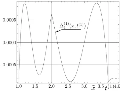
x∈A˜∆ (1)
Figure 1.Graph of the function∆(11)(x˜,t(1)).
for allt6=t(1). Second, we determined(1)1 such that
139
max
˜
x∈A˜ ∆ (1) 1 (x,˜ t
(1),d(1)
1 ) =−min ˜
x∈A˜∆ (1) 1 (x,˜ t
(1),d(1)
1 ). (4.6)
Thus we have
140
max
˜
x∈A˜ |∆ (1)
1 (x,˜ t(1),d (1)
1 )|6max ˜
x∈A˜ |∆ (1)
1 (x,˜ t,d1)| (4.7)
for all reald1andt∈(2, 4).∆(1)1 (x,˜ t)is an increasing function of ˜δ1(x,˜ t), hence 141
−d
(1)
1 −2 maxx˜∈A˜|δ˜1(x,˜ t(1)1 )|
2−d(1)1
= d
(1) 1
2−d(1)1 , (4.8)
which is satisfied for
142
d1(1)=max
˜
x∈A˜
|δ˜1(x,˜ t1(1))|=δ˜1 max. (4.9)
Thus we can find the maximum error of the first correction∆(1)1 (x,˜ t(1)1 )(presented at Fig.1):
143
max
˜
x∈A˜ |∆ (1)
1 (x,˜ t(1))|=
maxx˜∈A˜|δ˜1(x,˜ t(1))|
2−maxx˜∈A˜|δ˜1(x,˜ t(1))|
, (4.10)
which assumes the minimum value fort(1)=t(1r):
∆(1) 1 max=
maxx˜∈A˜|δ˜1(x,˜ t(1r))|
2−maxx˜∈A˜|δ˜1(x,˜ t(1r))|
= δ˜1 max 2−δ˜1 max
'8.7636·10−4' δ˜1 max
2.00 . (4.11)
This result practically coincides with ˜δ
00
1 maxgiven by (3.9). 145
Analogously we can determine the value ofd(1)2 (assuming thatt=t(1)is fixed):
146
−d
(1)
2 −maxx˜∈A˜|∆1(1)2(x,˜ t(1))(3+∆(1)1 (x,˜ t(1)))|
2−d(1)2
= d
(1) 2
2−d(1)2 . (4.12) Now, the deepest minimum comes from the global maximum
147
max
˜
x∈A˜ |∆(1)2
1 (x,˜ t(1))(3+∆ (1)
1 (x,˜ t(1)))|=
2 ˜δ21 max(3−δ˜1 max)
(2−δ˜1 max)3
. (4.13)
Therefore we get
148
d(1)2 = δ˜
2
1 max(3−δ˜1 max)
(2−δ˜1 max)3
'1.15234·10−6, (4.14)
and the maximum error of the second correction is given by
149
∆(1) 2 max=
d2(1) 2−d(1)2
'5.76173·10−7' δ˜2 max
7.98 , (4.15)
which is very close to the value of ˜δ002 maxgiven by (3.15). 150
Thus we have obtained the algorithmInvSqrt1which looks likeInvSqrtwith modified values of
151
numerical coefficients.
152
1. floatInvSqrt1(floatx){
2. floatsimhalfnumber = 0.500438180f*x; 3. inti = *(int*) &x;
4. i = 0x5F375A86 - (i>>1); 5. y = *(float*) &i;
6. y = y*(1.50131454f - simhalfnumber*y*y);
7. y = y*(1.50000086f - 0.999124984f*simhalfnumber*y*y); 8. returny ;
9. }
ComparingInvSqrt1 withInvSqrtwe easily see that the number of algebraic operations inInvSqrt1
153
is greater by 1 (an additional multiplication in line 7, corresponding to the second iteration of the modified
154
Newton-Raphson procedure). We point out that magic constants forInvSqrtandInvSqrt1are the same.
155
5. Numerical experiments 156
The new algorithms were tested on the processor Intel Core i5-3470 using the compiler TDM-GCC
157
4.9.2 32-bit (then, in the case ofInvSqrt, the values of errors are practically the same as those obtained by
158
Lomont [38]). The same results were obtained also on Intel i7-5700. In this section we analyze rounding
159
errors for the codeInvSqrt1.
160
Applying algorithmInvSqrt1 we obtain relative errors characterized by “oscillations” with a center
161
slightly shifted with respect to the analytical solution, see Fig.2. Calculations were carried out for all
Figure 2. Solid lines represent function ∆(21)(x˜,t(1)). Its vertical shifts by±6·10−8 are denoted by dashed lines. Finally, dots represent relative errors for 4000 random valuesx∈(2−126, 2128)produced by algorithmsInvSqrt1.
Figure 3.Relative errorε(1)arising during thefloatapproximation of corrections ˜y22(x˜,t). Dots represent
errors determined for 2000 random values ˜x∈[1, 4). Solid lines represent maximum (maxi) and minimum
(mini) values of relative errors (intervals[1, 2)and[2, 4)were divided into 64 equal intervals, and then
numbersxof the typefloatsuch thatex ∈ [−126, 128). The range of errors is the same for all these
163
intervals (exceptex =−126):
164
∆(1)
2;N(x) =sqrt(x)∗InvSqrt1(x)−1.∈(∆
(1) 2,Nmin,∆
(1)
2,Nmax), (5.1)
where
∆2,(1)Nmin=−6.62·10−7, ∆(1)2,Nmax=6.35·10−7.
Forex=−126 the interval of errors is slightly wider:
[−6.72·10−7, 6.49·10−7].
This can be explained by the fact that the analysis presented in this paper is not applicable to subnormals
165
numbers, see (2.1). The observed blur can be noticed already for the approximation error of the correction
166
˜ y22(x˜): 167
ε(1)(x˜) = InvSqrt1(x)−y˜22(x,˜ t (1))
˜
y22(x,˜ t(1))
. (5.2)
The values of this error are distributed symmetrically around the mean valuehε(1)i: 168
hε(1)i=2−1Nm−1
∑
x∈[1,4)
ε(1)(x˜) =−1.398·10−8 (5.3)
enclosing the range:
169
ε(1)(x˜)∈[−9.676·10−8, 6.805·10−8], (5.4)
see Fig.3. The blur parameters of the functionε(1)(x,˜ t)show that the main source of the difference 170
between analytical and numerical results is the use of precisionfloatand, in particular, rounding of
171
constant parameters of the function InvSqrt1. It is worthwhile to point out that in this case the amplitude
172
of the error oscillations is about 40% greater than the amplitude of oscillations of(y˜00−y˜0)/ ˜y0(i.e., in 173
the case ofInvSqrt), see the right part of Fig. 2 in [46].
174
6. Conclusions 175
In this paper we have presented a modification of the famous codeInvSqrtfor fast computation of
176
the inverse square root. The new code has the same magic constant but the second part (which consists
177
of Newton-Raphson iterations) is modified. In the case of one Newton-Raphson iteration the new code
178
InvSqrt1has the same computational cost asInvSqrtand is 2 times more accurate. In the case of two
179
iterations the computational cost of the new code is sligtly higher but its accuracy is higher by 8 times.
180
The main idea of our work consists in modifying coefficients in the Newton-Raphson method and
181
demanding that the maximal error is as small as possible. Such modifications can be constructed if the
182
distribution of errors for Newton-Raphson corrections is not symmetric (like in the case of the inverse
183
square root, when they are non-positive functions).
184
Author Contributions: Conceptualization, Leonid V. Moroz; Formal analysis, Cezary J. Walczyk; Investigation,
185
Cezary J. Walczyk, Leonid V. Moroz and Jan L. Cie´sli ´nski; Methodology, Cezary J. Walczyk and Leonid V. Moroz;
186
Visualization, Cezary J. Walczyk; Writing–original draft, Jan L. Cie´sli ´nski; Writing–review & editing, Jan L. Cie´sli ´nski
187
Funding:This research received no external funding.
188
Conflicts of Interest:The authors declare no conflict of interest.
References 190
1. M.D. Ercegovac, T. Lang:Digital Arithmetic, Morgan Kaufmann 2003.
191
2. B. Parhami:Computer Arithmetic: Algorithms and Hardware Designs, 2ndedition, Oxford Univ. Press, New York,
192
2010
193
3. K. Diefendorff, P. K. Dubey, R. Hochsprung, H. Scales: AltiVec extension to PowerPC accelerates media
194
processing,IEEE Micro20 (2) (2000) 85-95.
195
4. D. Harris: A Powering Unit for an OpenGL Lighting Engine,Proc. 35th Asilomar Conf. Singals, Systems, and 196
Computers(2001), pp. 1641–1645.
197
5. M. Sadeghian, J. Stine: Optimized Low-Power Elementary Function Approximation for Chybyshev series
198
Approximation,46th Asilomar Conf. on Signal Systems and Computers, 2012.
199
6. D. M. Russinoff: A Mechanically Checked Proof of Correctness of the AMD K5 Floating Point Square Root
200
Microcode,Formal Methods in System Design14 (1) (1999) 75–125.
201
7. M.Cornea, C. Anderson, C. Tsen: Software Implementation of the IEEE 754R Decimal Floating-Point Arithmetic,
202
Software and Data Technologies(Communications in Computer and Information Science, vol. 10), Springer 2008, pp.
203
97–109.
204
8. J.-M. Muller, N. Brisebarre, F. Dinechin, C.-P. Jeannerod, V. Lefèvre, G. Melquiond, N. Revol, D.Stehlé, S.
205
Torres: Hardware Implementation of Floating-Point Arithmetic,Handbook of Floating-Point Arithmetic(2009), pp.
206
269–320.
207
9. J.-M. Muller, N. Brisebarre, F. Dinechin, C.-P. Jeannerod, V. Lefèvre, G. Melquiond, N. Revol, D.Stehlé, S. Torres:
208
Software Implementation of Floating-Point Arithmetic,Handbook of Floating-Point Arithmetic(2009), pp. 321–372.
209
10. T. Viitanen, P. Jääskeläinen, O. Esko, J. Takala: Simplified floating-point division and square root, Proc. IEEE Int.
210
Conf. Acoustics Speech and Signal Process., pp. 2707–2711, May 26–31 2013.
211
11. M.D. Ercegovac, T. Lang: Division and Square Root: Digit Recurrence Algorithms and Implementations, Boston:
212
Kluwer Academic Publishers, 1994.
213
12. W. Liu, A. Nannarelli: Power Efficient Division and Square root Unit,IEEE Trans. Comp.61 (8) (2012) 1059–1070.
214
13. L.X. Deng, J.S. An: A low latency High-throughput Elementary Function Generator based on Enhanced double
215
rotation CORDIC,IEEE Symposium on Computer Applications and Communications (SCAC), 2014.
216
14. M. X. Nguyen, A. Dinh-Duc: Hardware-Based Algorithm for Sine and Cosine Computations using Fixed Point
217
Processor,11th International Conf. on Electrical Engineering/Electronics Computer, Telecommuncations and Information 218
Technology, IEEE 2014.
219
15. M. Cornea, IntelR AVX-512 Instructions and Their Use in the Implementation of Math Functions, Intel
220
Corporation 2015.
221
16. H. Jiang, S. Graillat, R. Barrio, C. Yang: Accurate, validated and fast evaluation of elementary symmetric
222
functions and its application,Appl. Math. Computation273 (2016) 1160–1178.
223
17. A. Fog: Software optimization resources, Instruction tables: Lists of instruction latencies, throughputs and
224
micro-operation breakdowns for Intel, AMD and VIA CPUs, http://www.agner.org/optimize/
225
18. L. Moroz, W. Samotyy: Efficient floating-point division for digital signal processing application,IEEE Signal 226
Processing Magazine36 (1) (2019) 159–163.
227
19. D.H. Eberly:GPGPU Programming for Games and Science, CRC Press 2015.
228
20. N. Ide, M. Hirano, Y. Endo, S. Yoshioka, H. Murakami, A. Kunimatsu, T. Sato, T. Kamei, T. Okada, M. Suzuoki:
229
2.44-GFLOPS 300-MHz Floating-Point Vector-Processing Unit for High-Performance 3D Graphics Computing,
230
IEEE J. Solid-State Circuits35 (7) (2000) 1025-1033.
231
21. S. Oberman, G. Favor, F. Weber: AMD 3DNow! technology: architecture and implementations,IEEE Micro19
232
(2) (1999) 37-48.
233
22. T.J. Kwon, J. Draper: Floating-point Division and Square root Implementation using a Taylor-Series Expansion
234
Algorithm with Reduced Look-Up Table, 51st Midwest Symposium on Circuits and Systems, 2008.
235
23. T.O. Hands, I. Griffiths, D.A. Marshall, G. Douglas: The fast inverse square root in scientific computing,Journal 236
of Physics Special Topics10 (1) (2011) A2-1.
24. J. Blinn: Floating-point tricks,IEEE Comput. Graphics Appl. 17 (4) (1997) 80-84.
238
25. J. Janhunen: Programmable MIMO detectors, PhD thesis, University of Oulu, Tampere 2011.
239
26. J.L.V.M. Stanislaus, T. Mohsenin: High Performance Compressive Sensing Reconstruction Hardware with QRD
240
Process, IEEE International Symposium on Circuits and Systems (ISCAS’12), May 2012.
241
27. Q. Avril, V. Gouranton, B. Arnaldi: Fast Collision Culling in Large-Scale Environments Using GPU Mapping
242
Function, ACM Eurographics Parallel Graphics and Visualization, Cagliari, Italy (2012).
243
28. R. Schattschneider: Accurate high-resolution 3D surface reconstruction and localisation using a wide-angle flat
244
port underwater stereo camera, PhD thesis, University of Canterbury, Christchurch, New Zealand, 2014.
245
29. S. Zafar, R. Adapa: Hardware architecture design and mapping of “Fast Inverse Square Root’s algorithm”,
246
International Conference on Advances in Electrical Engineering (ICAEE), 2014, pp. 1-4.
247
30. T. Hänninen, J. Janhunen, M. Juntti: Novel detector implementations for 3G LTE downlink and uplink,Analog. 248
Integr. Circ. Sig. Process.78 (2014) 645–655.
249
31. Z.Q. Li, Y. Chen, X.Y. Zeng: OFDM Synchronization implementation based on Chisel platform for 5G research,
250
2015 IEEE 11th International Conference on ASIC (ASICON).
251
32. C.J. Hsu, J.L. Chen, L.G. Chen: An Efficient Hardware Implementation of HON4D Feature Extraction for
252
Real-time Action Recognition, 2015 IEEE International Symposium on Consumer Electronics (ISCE).
253
33. C.H. Hsieh, Y.F. Chiu, Y.H. Shen, T.S. Chu, Y.H. Huang: A UWB Radar Signal Processing Platform for Real-Time
254
Human Respiratory Feature Extraction Based on Four-Segment Linear Waveform Model,IEEE Trans. Biomed. 255
Circ. Syst.10 (1) (2016) 219–230.
256
34. J.D. Lv, F. Wang, Z.H. Ma: Peach Fruit Recognition Method under Natural Environment, Eighth International
257
Conference on Digital Image Processing (ICDIP 2016), Proc. of SPIE Vol. 10033, edited by C.M.Falco, X.D.Jiang,
258
1003317 (29 August 2016).
259
35. D. Sangeetha, P. Deepa: Efficient Scale Invariant Human Detection using Histogram of Oriented Gradients for
260
IoT Services, 2017 30th International Conference on VLSI Design and 2017 16th International Conference on
261
Embedded Systems, p. 61–66, IEEE 2016.
262
36. J. Lin, Z.G. Xu, A. Nukada, N. Maruyama, S. Matsuoka: Optimizations of Two Compute-bound Scientific
263
Kernels on the SW26010 Many-core Processor, 46th International Conference on Parallel Processing, p. 432–441,
264
IEEE 2017.
265
37. id software, quake3-1.32b/code/game/q_math.c , Quake III Arena, 1999.
266
38. C. Lomont, Fast inverse square root, Purdue University, Tech. Rep., 2003. Available online:
267
http://www.lomont.org/Math/Papers/2003/InvSqrt.pdf.
268
39. H.S. Warren:Hacker’s delight, second edition, Pearson Education 2013.
269
40. P. Martin: Eight Rooty Pieces,Overload Journal135 (2016) 8–12.
270
41. M. Robertson: A Brief History of InvSqrt, Bachelor Thesis, Univ. of New Brunswick 2012.
271
42. B. Self: Efficiently Computing the Inverse Square Root Using Integer Operations. May 31, 2012.
272
43. C. McEniry: The Mathematics Behind the Fast Inverse Square Root Function Code, Tech. rep. 2007.
273
44. D. Eberly: An approximation for the Inverse Square Root Function, 2015, Available online:
274
http://www.geometrictools.com/Documentation/ApproxInvSqrt.pdf.
275
45. P. Kornerup, J.-M. Muller: Choosing starting values for certain Newton-Raphson iterations,Theor. Comp. Sci. 276
351 (2006) 101–110.
277
46. L. Moroz, C.J. Walczyk, A. Hrynchyshyn, V. Holimath, J.L. Cie´sli ´nski: Fast calculation of inverse square root
278
with the use of magic constant – analytical approach,Appl. Math. Computation316 (2018) 245–255.