Liquid Sloshing in Containers with Flexibility

(1)

Liquid Sloshing in Containers with

Flexibility

A thesis submitted in fulfillment of the

requirements for the degree of Doctor of

Philosophy

School of Engineering and Science

Faculty of Health, Engineering and Science Victoria University

Melbourne, Australia

by

Marija Gradinscak

(2)

Summary

Sloshing is the low frequency oscillations of the free surface of a liquid in a

partially filled container. The dynamic response of structures holding the liquid

can be significantly influenced by these oscillations, and their interaction with the

sloshing liquid could lead to instabilities. It is critical to predict and to control

sloshing in order to maintain safe operations in many engineering applications,

such as in-ground storage and marine transport of liquid cargo, aerospace vehicles

and earthquake-safe structures.

Contributions to the state of knowledge in predicting and controlling sloshing are

the main objectives of the proposed research. To this end, a numerical model has

been developed to enable reliable predictions of liquid sloshing. The numerical

results are compared with experimental results to determine the accuracy of the

numerical model. Further, the research addresses the employment of intentionally

induced sloshing to control structural oscillations. The novelty of this research is

in its use of a flexible container. Results indicate that intentionally introduced

flexibility of the container is capable of producing effective control. The practical

application of the proposed research is in the early design stages of engineering

(3)

Declaration

I, Marija Gradinscak, declare that the PhD thesis entitled Liquid Sloshing in

Containers with Flexibility is no more than 100,000 words in length including

quotes and exclusive of tables, figures, appendices, bibliography, references and

footnotes. This thesis contains no material that has been submitted previously, in

whole or in part, for the award of any other academic degree or diploma. Except

where otherwise indicated, this thesis is my own work.

Signature: Date:

(4)

The research and execution of this thesis would not have been possible without

the support, advice and comments from those who have taken the time to either

contribute or inquire into what has been keeping me busy for the last few years. I

am grateful for every person with whom I have discussed the subject for in some

way they have each contributed to the end result of this thesis.

Special acknowledgment must go to my supervisors; Associate Professor Özden

F. Turan and Dr Eren S. Semercigil for their encouragement and guidance during

the course of this investigation. For the generous contribution of their time during

the preparation of the draft, I am extremely grateful.

Thanks also go to my parents, Nikola and Tinka for creating the opportunity for

me to pursue this path. Great thanks to my son Marin and daughter Mariana for

supporting me in a difficult time.

And finally I would like to dedicate this thesis to my late husband Zlatko who

encouraged and supported my passion and gave me the strength and belief to

(5)

List of Illustrations

Figure 1.1:

Liquid sloshing in a rigid container

1

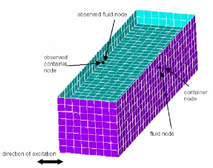
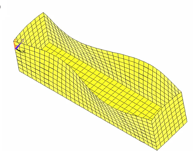
Figure 2.3.1:

The numerical model and the location of the observed nodes

15

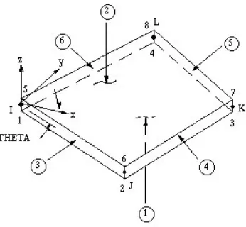
Figure 2.3.2:

Two-dimensional rectangular shell finite element.

16

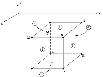
Figure 2.3.3:

Three-dimensional brick finite element.

17

Figure 2.3.4:

Structural mass element.

18

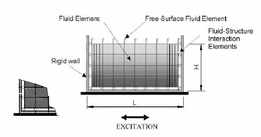
Figure 2.3.5:

Liquid-Structure interaction model

18

Figure 2.4.1:

Mode shapes of oscillation for the container with no added masses and no liquid.

21

Figure 2.4.1.1:

Predicted displacement histories of chosen fluid and structure nodes in a flexible container with various added masses, for the 25 mm mesh size runs. Added mass amounts: (a) 0 kg, (b) 5 kg, (c) 9 kg, (d) 13 kg.

23

Figure 2.4.1.2:

Predicted sloshing amplitude of chosen fluid nodes in a flexible container with various added masses, for the 25 mm mesh size runs. Added mass amounts: (a) 0 kg, (b) 5 kg, (c) 9 kg, (d) 13 kg.

24

Figure 2.4.1.3:

FFT plot of sloshing liquid (dashed-line) and structural vibration (solid-line) with various added masses, for the 25 mm mesh size runs. Added mass amounts: (a) 0 kg, (b) 5 kg, (c) 9 kg, (d) 13 kg.

25

Figure 2.4.1.4 Same as in Figure 2.4.1.1 but for the 50 mm mesh size runs and 10 ms time steps.

26

27

28

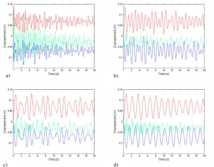
Figure 2.4.1.7: Predicted displacement histories of chosen fluid and

structure nodes in a flexible container with various added masses, for the 25 mm mesh size and 10ms time steps runs. Point mass amounts: (a) 0 kg, (b) 5 kg, (c) 9 kg, (d) 13 kg.

29

Figure 2.4.1.8: Predicted sloshing amplitude of chosen fluid nodes in a flexible container with various added masses, for the 25 mm mesh size and 10 ms time step runs. Point mass amounts: (a) 0 kg, (b) 5 kg, (c) 9 kg, (d) 13 kg.

30

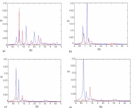
Figure 2.4.1.9: FFT plot of sloshing liquid (red-line) and structural vibration (blue-line) with various added masses, for the 25 mm mesh size and 10 ms time step runs. Point mass amounts: (a) 0 kg, (b) 5 kg, (c) 9 kg,

(8)

Figure 2.4.1.11: Same as in Figure 2.4.1.8 but for the 25 mm mesh size and

5 ms time step run. 33

Figure 2.4.1.12: Same as in Figure 2.4.1.8 but for the 25 mm mesh size and

5 ms time step run. 34

Figure 2.4.2:

Displacement histories of the liquid in a flexible container with 1mmwallthickness and no added mass (a).The liquid is undamped and structure has 1% damping. Predicted sloshing amplitude for the same case (b). Corresponding frequency spectrum of sloshing liquid (red) and structure (blue) (c).

36

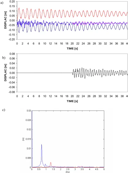
Figure2.4.3:

Displacement histories of the liquid in a flexible container with 1 mm wall thickness and 9 kg added mass (a).The liquid is undamped and structure has 1% damping. Predicted sloshing amplitude for the same case (b). Corresponding frequency spectrum of sloshing liquid (red) and structure (blue) (c).

37

Figure 2.4.4:

Displacement histories of the liquid in a flexible container with 1 mm wall thickness and 13 kg added mass (a).The liquid is undamped and structure has 1% damping. Predicted sloshing amplitude for the same case (b). Corresponding frequency spectrum of sloshing liquid (red) and structure (blue) (c).

38

Figure 2.5.1:

(a)Predicted absolute displacement histories of the liquid in a rigid container, (b) sloshing amplitude for the same case, (c) corresponding displacement frequency spectrum of sloshing liquid.

42

Figure 2.5.2:

(a) Predicted displacement histories of the liquid in a flexible container with 1mm wall thickness and0 kg added mass, (b) sloshing history, (c) frequency

spectrum of sloshing liquid (——) and structure (——), (d)

cross-correlation between container wall displacement and liquid sloshing and (d) its frequency spectrum. The liquid is undamped and structure has 1% damping.

46

Figure2.5.3:

(a) Predicted displacement histories of the liquid in a flexible container with 1mm wall thickness and 3 kg added mass, (b) sloshing history, (c) frequency spectrum of sloshing liquid (——) and structure (——), (d) cross-correlation between container wall displacement and liquid sloshing and (d) its frequency spectrum. The liquid is undamped and structure has 1% damping.

48

Figure 2.5.4:

(9)

Figure 2.5.5:

54

Figure 2.5.6:

56

Figure 2.5.7:

59

Figure 2.5.8.

Variation of the rms of sloshing magnitude in m with mass for rigid (▬▬) and flexible () containers.

60

Figure 2.5.9.

Probability distribution for sloshing in rigid container ( ▌) and flexible container with 9 kg added mass ( ▌).

61

Figure 2.6.1:

Schematic view of the experimental setup for the base excitation. 1: personal computer, 2: power amplifier, 3: electromagnetic shaker, 4: container.

62

Figure 2.6.2:

Absolute sloshing magnitude in m with mass for rigid (▬▬) and flexible () containers.

64

Figure 3.2.1:

The numerical model and the location of straps and observation nodes. 70

Figure 3.2.2:

Finite Element-Straps. 71

Figure 3.3.1:

Mode shapes of oscillation for the container with straps on the top and no liquid.

74

Figure 3.4.1:

Displacement histories of the liquid in a flexible container with three straps on top, 1mm wall thickness and 0 kg added mass (a). The liquid is undamped and structure has 1% damping. Predicted sloshing amplitude for the same case (b). The frequency spectra of the container displacement (blue) and sloshing (red) are presented (c).

76

(10)

the same case (b). The frequency spectra of the container displacement (blue) and sloshing (red)are presented (c).

Figure 3.4.3:

Displacement histories of the liquid in a flexible container with three straps on top, 1mm wall thickness and 5kg added mass (a). The liquid is undamped and structure has 1% damping. Predicted sloshing amplitude for the same case (b). The frequency spectra of the container displacement (blue) and sloshing (red)are presented (c).

81

Figure 3.4.4:

82

Figure 3.4.5:

83

Figure 3.4.6:

85

Figure 3.4.7:

86

Figure 3.4.8:

Variation of rms sloshing amplitude with added mass for cases: rigid container (――), flexible container without () and flexible container with (z) straps.

87

Figure 3.5:

Absolute sloshing amplitude with added mass for cases: rigid container (――), flexible container with () straps.

88

Figure 4.3.1:

Showing (a) the computational model and (b) the displacement history of the structure after an initial displacement.

97

Figure 4.3.2:

Three dimensionalsolid structure element (ANSYS 2002)

99

Figure 4.3.3:

(11)

Figure 4.4.1:

a) numerically predicted displacement histories of the sloshing absorber: liquid displacement histories in container with rigid walls. b) predicted sloshing amplitude, c) structure displacement and d) FFT of sloshing liquid (red) and plate displacement (green).

102

Figure 4.4.2:

a) numerically predicted displacement histories of the container walls and liquid. b) predicted sloshing amplitude in flexible container with 9 kg added mass, c) structure displacement and d) FFT of wall displacement (blue), sloshing liquid (red) and plate displacement (green).

105

Figure 4.4.3:

107

Figure 4.4.4:

108

Figure 4.4.5:

110

Figure 4.4.6:

111

Figure 4.4.7:

112

Figure 4.4.8:

113

Figure 4.4.1.1:

a) numerically predicted displacement histories of the container walls and liquid. b) predicted sloshing amplitude in flexible container with 0 kg point mass, c) structure displacement and d) FFT of wall displacement (blue), sloshing liquid (red) and plate displacement (green). Liquid is undamped and container has 5% damping.

115

Figure 4.4.1.2:

(12)

and container has 5% damping. Figure 4.4.1.3:

118

Figure 4.4.1.4:

120

Figure 4.4.1.5:

121

Figure 4.4.1.6:

122

Figure 4.4.9:

Variations of the rms of (a) sloshing amplitude and (b) structure’s displacement. (▬▬ structure alone, ▬▬ rigid container; and flexible container with structural damping of 1.5% , 5% and S 10%) .

123

Figure 4.4.2.1:

a) numerically predicted displacement histories of the container walls and liquid. b) predicted sloshing amplitude in flexible container with no added mass, c) structure displacement and d) FFT of wall displacement (blue), sloshing liquid (red) and plate displacement (green). The mass of the structure is 1500 kg.

126

Figure 4.4.2.2:

a) numerically predicted displacement histories of the container walls and liquid. b) predicted sloshing amplitude in flexible container with 9 kg added mass, c) structure displacement and d) FFT of wall displacement (blue), sloshing liquid (red) and plate displacement (green). The mass of the structure is 1500 kg.

127

Figure 4.4.2.3:

a) numerically predicted displacement histories of the container walls and liquid. b) predicted sloshing amplitude in flexible container with 13 kg added mass, c) structure displacement and d) FFT of wall displacement (blue), sloshing liquid (red) and plate displacement (green). The mass of the structure is 1500 kg.

(13)

Figure 4.4.2.4:

a) numerically predicted displacement histories of the container walls and liquid. b) predicted sloshing amplitude in flexible container with 0 kg point mass, c) structure’s displacement and d) FFT of wall displacement (blue), sloshing liquid (red) and plate displacement (green). The mass of the structure is 1000 kg.

129

Figure 4.4.2.5:

a) numerically predicted displacement histories of the container walls and liquid. b) predicted sloshing amplitude in flexible container with 9 kg point mass, c) structure’s displacement and d) FFT of wall displacement (blue), sloshing liquid (red) and plate displacement (green). The mass of the structure is 1000 kg.

130

Figure 4.4.2.6:

a) numerically predicted displacement histories of the container walls and liquid. b) predicted sloshing amplitude in flexible container with 13 kg point mass, c) structure’s displacement and d) FFT of wall displacement (blue), sloshing liquid

131

Figure 4.4.10:

Variations of the rms of (a) sloshing amplitude and (b) structural displacement. (▬) rigid container; and flexible container with mass ratio of 2000 kg , 1500 kg and S 1000 kg).

(14)

Table 2.4.1:

First, second and third natural frequencies of the container without liquid for different masses. Selective cases were experimentally verified at the fundamental mode.

22

Table 2.6.1:

Observed liquid surface vertical peak displacement.

64

Table 3.3.1: First, second and third natural frequencies of the

(15)

Chapter 1

Introduction

The liquid surface in a partially full container can move back and forth (in standing or

traveling waves) at discrete natural frequencies. This low frequency oscillation of the

liquid is defined as sloshing. In Figure 1.1, L indicates the width of the container (also the

wavelength), and H the height of the static liquid level. The shaded area indicates the

expected shape of the free surface at its fundamental mode. Sloshing at the fundamental

frequency mobilizes the largest amount of liquid, and may produce excessive structural

loads that can lead to structural failure. Welt et al. (1992) showed that sloshing resulting

from external forces is critical when the excitation frequency is close to the fundamental

sloshing frequency.

(16)

engineering applications, such as in ground and marine transport of liquid cargo,

aerospace vehicles and earthquake–safe structures. Most commonly, the harmful effect of

sloshing is experienced in transportation and storage of liquid cargo, Popov et al. (1992).

In marine engineering, sloshing plays a significant role in defining maneuverability and

safety of vessels, Fotia et al. (2000).

The inherent flexibility of a liquid container is usually treated as a problem since

achieving a perfectly rigid container is a practical impossibility. Container flexibility, on

the other hand, may be treated as a design parameter to gain benefit, rather than a

nuisance to overcome. The novelty of the presented thesis is to investigate the required

flexibility parameters of a container to achieve either the suppression of its content or to

utilize intentionally induced sloshing as a vibration control agent for light and flexible

structures. To the best of the author’s knowledge, this is the first attempt to make use of

flexibility as a design parameter in the control of liquid sloshing. Most of the reported

efforts in this thesis are of numerical nature. Limited simple experiments are presented to

validate some of the numerical predictions.

The research in this thesis is divided into three areas. Firstly, the observations from

extensive numerical predictions of liquid sloshing in a container with flexible walls are

presented. Efforts are summarized to determine the tuning condition of the container

flexibility to the dynamics of sloshing liquid for effective sloshing control. Second area

of the focus deals with improving the design of the flexible container to facilitate

(17)

controlling structural vibrations. Hence, as mentioned earlier, the general objective in this

research is to explore the possibilities of using the flexibility of the container as a design

parameter. To clarify the specific objectives, a brief description of the content of each

chapter is given next. Each of these chapters is presented as a self-contained entity, with

its own relevant literature and conclusions.

Chapter 2 explores the possibility of using a container with flexible walls to control the

sloshing of its liquid content. The flexibility of a container may be employed to suppress

excessive sloshing only when there is a strong interaction between the container and the

liquid. This strong interaction is ideally achieved when the fundamental structural

frequency of the container, in the direction of sloshing, is tuned to the fundamental

sloshing frequency. However, this ideal condition may not be possible and multiple

vibration modes may be involved in the process, due to the structural complexity of the

container and strong fluid-structure interactions.

The flexible container used in this study has its critical frequencies higher than the

sloshing frequencies involved. Hence, tuning requires lowering the container frequencies.

The method chosen to lower these frequencies is to add mass to the container. Control in

the order of 80% has been demonstrated to be possible as compared to the sloshing levels

observed with a rigid container. The following list includes the published work relevant

to this chapter:

Gradinscak, M. Semercigil, S. E. and Turan, Ö. F., 2001, Sloshing Control with

Container Flexibility, 14th Australasian Fluid Mechanics Conference, Adelaide

(18)

Engineering Division Summer Meeting, Montreal, Quebec, Canada.

Güzel, U. B, Gradinscak, M., Semercigil, S. E. and Turan, Ö. F., 2004, Control of

Liquid Sloshing in Flexible Containers: Part 1. Added Mass, 15th Australasian Fluid

Mechanics Conference, University of Sydney, Sydney, Australia.

Güzel, U. B., Gradinscak, M., Semercigil, S. E. and Turan, Ö. F., 2005, Tuning Flexible

Containers for Sloshing Control, Proceedings of the IMAC-XXIII: A Conference and

Exposition on Structural Dynamics, January 31-February 3, Orlando, Florida.

Gradinscak, M., Semercigil, S. E. and Turan, Ö. F., 2006, Liquid Sloshing in Flexible

Containers, Part 1: Tuning Container Flexibility for Sloshing Control, Fifth International

conference on CFD in the Process Industries, CSIRO, Melbourne, Australia, 13-15

December.

Chapter 3 deals with improvement of the container design by adding auxiliary structural

elements to it. The motivation for this chapter comes from the observations made in

Chapter 2 when rather large structural deflections are required to achieve the reported

levels of sloshing control. These large deflections may be difficult to accommodate in

some practical applications. Hence, it is desirable to limit them while maintaining the

effectiveness of control.

Large deflections are observed at the open top of the container, away from the centre of

the container. Hence, rigid links (or straps) which are attached at the opposite sides of the

open top, may limit these outward deflections. Observations are reported in Chapter 3, to

limit the container deflections to practical levels, with almost identical levels of sloshing

(19)

Gradinscak, M., Güzel, U. B, Semercigil, S. E. and Turan, Ö. F., 2004, Control of

Liquid Sloshing in Flexible Containers: Part 2. Added Straps, 15th Australasian Fluid

Mechanics Conference, University of Sydney, Sydney, Australia.

Tuned liquid dampers may be employed for structural vibration control, similar to that of

a classical tuned vibration absorber. For such cases, the fundamental sloshing frequency

is tuned at a critical frequency of the structure to be controlled. The pressure forces, as a

result of the intentionally induced liquid sloshing, are used as control forces. Such an

absorber has the benefits of being effective and practically free of maintenance. The work

presented in Chapter 4 demonstrates the effects of container flexibility on structural

vibration control. The supression of structural response can improve by up to 80% as

compared to that can be obtained with a tuned sloshing absorber with a rigid container.

Work related to this chapter has been presented in:

Gradinscak, M. Semercigil, S. E. and Turan, Ö. F., 2006, Liquid Sloshing in Flexible

Containers, Part2: Using a Sloshing Absorber With a Flexible Container for Structural

Control, Fifth International conference on CFD in the Process Industries, CSIRO,

Melbourne, Australia, 13-15 December.

Chapter 5 of this thesis summarises the efforts presented in the earlier content chapters,

and presents recommendations to further the findings. Since the working principles of the

classical tuned vibration absorber is the starting point of most the presented material of

this thesis, Appendix A is allocated for a summary of tuned vibration absorbers, for

completeness. Appendix B presents results obtained in forty second time frames of the

(20)

displacement of the controlled structure. Appendix D presents the effect of different mass

(21)

Chapter 2

CONTROL OF LIQUID SLOSHING

USING A FLEXIBLE CONTAINER

2.1 Introduction

This chapter presents the outcomes of investigations conducted into the possibility of

using a container with flexible walls to achieve an effective control of liquid sloshing. It

is the primary contribution of this thesis to the state of knowledge. The chapter is

organized as follows:

• Section 2.2 presents the literature review of the relevant previous work

concerning liquid sloshing.

• Section 2.3 gives detailed explanations of the finite element model developed to

simulate liquid–flexible structure interaction.

• Section 2.4 deals with the further details of the numerical process.

• Section 2.5 discusses numerical observations.

• Section 2.6 outlines relevant experimental observations.

• Section 2.7 reiterates the primary findings on employing container flexibility in

(22)

Sloshing generally refers to the low-frequency oscillations of the free surface of a liquid

in a partially filled container. When liquid mass represents a large percentage of the total

mass of a structure, sloshing could induce disturbance to its stability. This is mainly

contributed to by the induced dynamic loads and shift of the centre of gravity.

The study of sloshing is critical both industrially and environmentally, thus attracting

research and academic literature which explores sloshing and attempts to control its

impact. Study of sloshing generally proves challenging due to the presence of strong flow

interactions with its container. These interactions become even more challenging if the

container is flexible. The primary cause of these greater complexities is the moving

boundaries of the fluid as the flexible container deforms under the effect of dynamic

sloshing loads. As a result, the dynamic responses of a flexible container may be

significantly different than that with rigid walls.

2.2.1 Literature Review

Early research on sloshing in flexible containers can be found in Kana and Abramson

(1966) which reports experiments to determine the response of a cylindrical elastic tank.

Experiments revealed nonlinearity in the deformation of the shell wall when the elastic

shell contained liquid with a free surface. High frequency, small amplitude vibration

excitation of the elastic structure, in a circumferential mode, led to a low frequency, large

amplitude free surface motion of the liquid, in a rotationally symmetric mode. The

(23)

were used in this reference, to obtain analytical solutions for restricted ranges of input

conditions.

Haroun and Housner (1981) and Veletos (1984) developed a mechanical model for

flexible tanks. The liquid-tank system was converted into an equivalent spring-mass

system which brought hydrodynamic simplification. Jain and Medhekar (1993a, 1993b)

draw attention to this mechanical model and suggest separate models for rigid and

flexible tanks. They recommend that the Haroun and Housner (1981) model be used for a

flexible tank, and Veletsos (1984) model to be used for a rigid tank. Malhotra et al.

(2000) continued to investigate the possibilities of simplification of the previously

developed flexible tank model, but their results are not significantly different from the

rigid container model. These mechanical models convert the container-liquid system into

an equivalent spring-mass system and considerably simplify the analyses.

Chen and Haroun (1994) and Jeong and Kim (1998) report investigations on container

flexibility with a primary interest to determine natural frequencies and mode shapes of

containers with liquid. Chen and Haroun (1994) report a numerical model for a

two-dimensional system consisting of a liquid and a flexible tank. The liquid was considered

to be inviscid, incompressible and irrotational. The model required the addition of

artificial energy dissipation to stabilize the numerical simulation. Jeong and Kim (1998)

present an analytical method for determining the natural frequency of shells filled with

liquid. In this research, liquid movement was restricted by rigid plates placed at the top

(24)

fluid elements for the sloshing fluid model.

Tang (1994) reports results of an investigation on the dynamic response of a tank

containing two different liquids under seismic excitation. Both analytical and numerical

approaches are considered. Research is based on assumptions that, in its fixed-base

condition, the tank-liquid system responds in its fundamental mode of vibration as a

single-degree-of-freedom system and that the convective component of the response is

not affected by the soil-structure-interaction.

Yao et al. (1994) develop a numerical model to simulate three-dimensional waves in

narrow tanks. Energy dissipation was added to match predicted wave amplitudes to

experimental data. Takahara et al. (1995) simulated sloshing of fluid in cylindrical tanks

subjected to pitching excitation at a frequency in the neighborhood of the lowest resonant

frequency. The nonlinearity of the liquid surface oscillation and the nonlinear coupling

between the dominant modes and other modes are considered in the response analysis of

the sloshing motion. The equations governing the amplitude of liquid surface motions are

derived and the stability analysis of each motion is conducted. Equivalent damping terms

were added to their formulation to account for the energy dissipation.

Movement of vessels containing liquid is a common operation in the packaging industry.

Yano et al. (2002) reported research on a container gradually accelerating on an inclined

path, paying special attention to the suppression of the sloshing. Garrido (2003)

investigates modeling efforts of sloshing in a rectangular container which is first

(25)

pendulum model and experiments are reported as satisfactory whilst acknowledging the

limitations of the simplicity of the model. Grundelius and Bernhardsson (2000)

investigate industrially relevant problems of movement of a carton container, from one

position to another in the packaging machine. An open container with liquid has to be

moved without excessive sloshing. It is acknowledged that the severity of sloshing

depends on how the package is accelerated and on the properties of the liquid. It proposes

an iterative learning control approach and attempts to find an open loop acceleration

reference using the obtained results in the next iteration with repeating the same

procedure until the desired outcome have been accomplished.

For flexible structures, only recently researchers begin to use the fully nonlinear theory to

explain more accurately the phenomenon of flow physics associated with liquid sloshing.

Pal et al. (2003) study non-linear free surface oscillation of a liquid inside elastic

containers using the finite element technique. The finite element method based on

two-dimensional fluid and structural elements is used for the numerical simulation. A

numerical scheme is developed on the basis of a mixed Eulerian–Lagrangian approach,

with velocity potential as the unknown nodal variable in the fluid domain and

displacements as unknowns in the structural domain. Numerical results obtained by this

investigation for rigid containers are first compared with existing solutions to validate the

code for non-linear sloshing without fluid–structure coupling. Bauer et al. (2004) employ

an elastic membrane in a rigid container, resulting in considerable reduction of liquid

sloshing. Although theoretical and numerical observations compare favorably, cases are

(26)

finite element method. Mitra and Sinhamahapatra (2005) present a new pressure-based

Galerkin finite element that could handle flexible walls, but the cases are restricted to

linear problems with small amplitude waves.

Anderson (2000) mentions for the first time, the possibility of using container flexibility

for the control of liquid sloshing. Numerical predictions show that the sloshing wave

amplitude can be significantly reduced by tuning the interaction of the flexible container

with liquid sloshing. Experiments were carried out to verify the numerical model.

Gradinscak et al. (2001, 2002 and 2006) and Guzel et al. (2004, 2005) report the design

potential of flexible containers for significant reduction of sloshing. The flexibility of a

container may be employed to suppress excessive sloshing only when there is a strong

interaction between the container and the liquid. This strong interaction is achieved when

the fundamental structural frequency, in the direction of the sloshing, is tuned to the

fundamental sloshing frequency of liquid. Throughout this thesis the research is discussed

in further detail.

2.2.2 Summary of literature review

In summary, the published work of the previous research has certainly provided direction

for further research throughout this thesis. The author gratefully acknowledges these

contributions. However, a good portion of the current research has been restricted to the

approximation, and unavoidable simplification, of the liquid sloshing problem. On the

other hand, the complexity of sloshing, such as non-linearity and ‘liquid-structure

(27)

solutions for control. Reporting of container flexibility as a design tool to control sloshing

has not been found in the literature. It is the intention of this thesis to explore such

possibility and demonstrate its promise.

In this thesis, the dynamic interaction of a flexible container and liquid sloshing is

utilized for the purpose of controlling liquid sloshing. The primary concern is the

reduction of liquid sloshing using container flexibility. This concept is a novel one. This

work is important in applications involving the storage and transportation of liquid goods

where sloshing can either damage the liquid product or compromise the structural

integrity of the container. In practice, the advantages of using a flexible container are two

fold. First, if sloshing of liquid is suppressed effectively, then the safety of the intended

operation is enhanced. Secondly, a flexible container is lighter than its rigid counterpart

which should result in cost reductions and material savings.

2.3 Numerical Model and Procedure

2.3.1 Description of the model and test conditions

ANSYS (2002) finite element analyses package was used to model the flexible container

and the sloshing liquid. The flexible container used for the numerical model was of

aluminium, an open top rectangular prism of 1.6 m in length, 0.4 m in width and 0.4 m in

height. The wall thickness was 1 mm. The container was filled with water to a depth of

0.3 m. The total weight of the container was 6 kg. The Young’s modulus, Poisson ratio

(28)

container was modeled with two-dimensional rectangular shell elements. Three

dimensional brick elements were used to model the liquid. Fluid-structure interaction was

achieved by coupling the liquid displacement with that of the container walls with

relative velocity vector in the direction of the normal equal to zero. Hence, the liquid was

constrained by the walls.

The objective of the simulation was to obtain the displacement histories at several

locations of both the container and liquid. Sloshing was induced by imposing a transient 5

mm – sinusoidal displacement of one cycle to the base of the container in y-direction, as

shown in Figure 2.3.1. The frequency of this disturbance was chosen to be 1.34 Hz,

which is the fundamental sloshing frequency of a rigid container of the same dimensions,

Milne-Thomson (1968). In Equation (1) below, a closed form expression is given of the

fundamental sloshing frequency, where h and d are the liquid height and container width,

respectively.

⎟

⎠

⎞

⎜

⎝

⎛

=

d

h

tanh

d

g

2

1 π

π

f

₍₁₎

The concept of using a flexible container to control sloshing of a liquid is similar to that

of using a tuned absorber to control excessive vibrations of a mechanical oscillator. For

completeness, a brief description of the tuned vibration absorber is given in Appendix A.

For a tuned absorber, the natural frequency of the absorber is tuned to that of the structure

to be controlled, to maintain minimum oscillation amplitudes, whilst this same absorber

(29)

the structure to be controlled, whereas the flexible container is expected to act like the

tuned absorber.

Tuning the container dynamics to that of the sloshing liquid is attempted by adding point

masses on the flexible container. Two masses are added directly above the “observed

container node” indicated in Figure 2.3.1, on the free edge of the flexible walls.

Figure 2.3.1: The numerical model and the location of the observed nodes.

The finite element model of the container was created using two-dimensional rectangular

shell elements, SHELL63 (ANSYS 2002) with the characteristics as shown in Figure

(30)

simulations for elastic and rigid definitions of the container. As outlined earlier, 0.001 m

(1 mm) wall thickness is assigned to the flexible container. This thickness was increased

to 0.005 m (5 mm) in order to predict the response of a rigid container having the same

dimensions as those of the flexible container.

Numerous trials were undertaken with the intention to verify grid cell size and its

explanation proceeds in this chapter. As an outcome from those trials, the grid cell size of

50mmx50mm was selected as sufficient for numerical accuracy for both container and

liquid models. The full finite element model of the container was discretised into 896

elements.

Figure 2.3.2: Two-dimensional rectangular shell finite element.

FLUID80 (ANSYS 2002), three-dimensional brick finite elements were used to model

the liquid. The total weight of the liquid content is 192kg. The brick finite element is

shown in Figure 2.3.3, which is defined by eight nodes having three degrees of freedom

at each node. The parameters for the finite element model were defined for a

(31)

The complex physical behavior of the free surface liquid utilizes formulations of

nonlinear wave theory and is defined by the gravity springs attached to each node of the

liquid. The full liquid finite element model was discretised into 1536 elements.

Figure 2.3.3: Three-dimensional brick finite element.

To control sloshing, the objective is to tune the container’s fundamental natural frequency

to the fundamental sloshing frequency. The tuning has been attempted by adding mass

elements at the top edge and in the middle of the 1.6 m long sides of the container. The

structural mass element, MASS21 (ANSYS 2002), is defined as a single node as shown

(32)

Liquid boundary conditions are shown in Figure 2.3.5. These boundary conditions have

been defined using separate coincident nodes for each liquid element. These nodes were

then coupled with the structural elements in the direction normal to the interface.

(33)

2.4 Computational Simulations

The dynamic response and natural frequencies of both the liquid and the container are

influenced by strong interactions between them. The strong interaction between liquid

and container is achieved when the fundamental frequency of the liquid (in the direction

of sloshing) is tuned to the fundamental frequency of the container.

The response of the container’s structure depends primarily on its natural frequencies,

damping characteristics, and the frequency content of the time-varying loads. Eigenvalue

modal analysis has been used first to determine the container’s natural frequencies and

mode shapes. Three mode shapes of oscillation of the container are obtained and given in

Figure 2.4.1. Natural frequencies for different added masses are determined and are given

in Table 2.4.1.

The first mode shape of oscillation, in Figure 2.4.1 (a), shows that oscillations along the

longest walls of the container are out of phase. The second mode shape of oscillation in

Figure 2.4.1 (b), shows that the oscillations along the longest walls are in phase, whilst

the third and higher modes showed much clearer separation of frequencies, Figure 2.4.1

(c). The first and second modes are plate modes with the first one an out-of-phase mode,

(34)

(35)

Figure 2.4.1.: Mode shapes of oscillation for the container with 0 kg point mass and no liquid.

From Table 2.4.1, the frequency for the simulation without mass is significantly higher

than the theoretical fundamental sloshing frequency of liquid, which is calculated at 1.34

Hz. By adding masses those natural frequencies of the container become closer to

sloshing frequency. However, it should be remembered that the frequencies changed

when container contained liquid. Hence, the information in Figure 2.4.1 and Table 2.4.1

(36)

Mass [kg] 1st _natural

frequency [Hz]

2nd _natural

frequency [Hz]

3rd _natural

frequency [Hz]

0 6.38 6.47 9.25

3 1.41 1.42 9.25

5 1.1 1.1 9.25

7 0.94 0.94 9.25

9 0.83 0.83 9.25

11 0.75 0.75 9.25 13 0.69 0.69 9.25

2.4.1Selection of Mesh Size

As mentioned earlier in this chapter, the container walls have been represented with

standard shell elements in the FEA model. 3-D fluid elements have been used for the

liquid in the container. The container is meshed with square elements of 0.05 m x 0.05 m

size and the liquid is meshed with cubic elements of 0.05 m x 0.05 m x 0.05 m size. The

solution is independent of the mesh size at this resolution. Grid independence has been

verified by testing 0.025 m square and cubic elements for the same selected cases of forty

(37)

Figure 2.4.1.1: Predicted displacement histories of chosen fluid and structure nodes in a flexible container with various added masses, for the 25 mm mesh size and 10 ms time steps runs. Point mass amounts: (a) 0 kg, (b) 5 kg, (c) 9 kg, (d) 13 kg.

Figure 2.4.1.1 gives the displacement histories of the container and fluid nodes for 0.025

m mesh size tests. Figure 2.4.1.4 gives the displacement histories of the container and

fluid nodes for 0.05 m mesh size tests. Top and bottom solid lines in red and blue indicate

the container nodes. Dashed lines in the middle in green indicate the fluid node

displacement histories. Very similar displacement patterns are seen in Figure 2.4.1.1 with

0.025 m mesh, in comparison to Figure 2.4.1.4 with 0.05 m mesh, for 0 kg, 5 kg, 9 kg, 13

kg added point masses cases, respectively, indicating negligible difference between 0.025

m and 0.05 m mesh sizes.

a) b)

(38)

Figure 2.4.1.2: Predicted sloshing amplitude of chosen fluid nodes in a flexible container with various added masses, for the 25 mm mesh size and 10 ms time steps runs. Point mass amounts: (a) 0 kg, (b) 5 kg, (c) 9 kg, (d) 13 kg.

Sloshing amplitudes for the selected cases with 0.025 m mesh size are shown in Figure

2.4.1.2. Figure 2.4.1.5 gives the sloshing amplitude for 0.05 m mesh size tests. The high

sloshing amplitude around 0.05 m for the case with 0 kg point mass is gradually

decreasing until the 9 kg point mass case in Figure 2.4.1.2 (c) to a level just below 0.02

m. The tuning effect is assumed to be lost beyond this point as seen in Figure 2.4.1.2 (d),

where sloshing amplitude is increasing back to above 0.02 m. Figure 2.4.1.5 give the

same sloshing histories obtained with the 0.05 m mesh size. Differences between

respective plots for the selected cases are again insignificant.

(39)

Figure 2.4.1.3: FFT plot of sloshing liquid (red-line) and structural vibration (blue-line) with various added masses, for the 25 mm mesh size and 10 ms time steps runs. Point mass amounts: (a) 0 kg, (b) 5 kg, (c) 9 kg, (d) 13 kg.

The FFT plots of liquid sloshing and structural vibration data for 0.025 m mesh size are

given in Figure 2.4.1.3. The FFT plots of liquid sloshing and structural vibration data for

0.05 m mesh size are given in Figure 2.4.1.6. Red line indicates sloshing, and blue line

indicates structural spectral distributions. The horizontal axis represents frequency in

[Hz] and the vertical axis represents spectral magnitude [m]. All spectral plots presented

in this section and for the rest of this thesis are single-sided.

a) _b)

(40)

The sloshing frequencies are dominant in Figure 2.4.1.3 (a), around 1.2 Hz and 1.4 Hz.

The main structural frequencies that are around 0.8 Hz, 1.2 Hz and 1.75 Hz are lesser in

magnitude. By looking at the highest peak around 1.2 Hz attributed to sloshing, it is

possible to say that the structure is driven by the fluid. The addition of 5 kg and then 9 kg

point masses in Figures 2.4.1.3 (b) and (c) seems to transform the system to one that is

structurally driven, as opposed to one driven by the sloshing. The structural peak around

1.3 Hz in Figure 2.4.1.3 (b) which then shifts to 1.1 Hz in Figure 2.4.1.3 (c) is clearly

suppressing the sloshing peaks in this range.

(41)

The same observation can be made for the other major structural peak around 0.8Hz and

0.75 Hz for 5 kg and 9 kg point mass cases respectively. Again by looking at Figure

2.4.1.3 (d) it is possible to see that the fluid and the structure are not effectively

controlling each other any more. Rather they are both acting in their separate ranges, -

structure around 0.7 Hz and sloshing around 1.4 Hz.

c) d)

(42)

0 0.5 1 1.5 2 2.5 3 3.5 4 4.5 5 0

0.005 0.01 0.015 0.02

(Hz)

(m

)

0 0.5 1 1.5 2 2.5 3 3.5 4 4.5 5

0 0.005 0.01 0.015 0.02

(Hz)

(m

)

0 0.5 1 1.5 2 2.5 3 3.5 4 4.5 5

0 0.005 0.01 0.015 0.02 0.025 0.03

(Hz)

(m

)

0 0.5 1 1.5 2 2.5 3 3.5 4 4.5 5

0 0.005 0.01 0.015 0.02 0.025 0.03

(Hz)

(m

)

The FFT plots of 0.0550 m mesh size are given in Figure 2.4.1.6. It can be observed that

it is possible to predict the same behavior with 50 mm mesh size as that for the 25 mm

mesh. This leads to the conclusion that obtained results with a finer mesh are very similar

to the results of the chosen mesh size.

a) b)

(43)

2.4.2 Time Step Size

A transient analysis has been conducted with 10 milliseconds (ms) time step. These 10

ms time steps were selected as there was minimal difference between 10 ms and 5 ms

time steps, to be more cost effective. For verification, 25 mm mesh size run and 10 ms

time step for the same selected cases have been presented here in Figures 2.4.1.7, 2.4.1.8

and 2.4.1.9

Figure 2.4.1.7: Predicted displacement histories of chosen fluid and structure nodes in a flexible container with various added masses, for the 25 mm mesh size and 10ms time steps runs. Point mass amounts: (a) 0 kg, (b) 5 kg, (c) 9 kg, (d) 13 kg.

a) b)

(44)

Figure 2.4.1.8: Predicted sloshing amplitude of chosen fluid nodes in a flexible container with various added masses, for the 25 mm mesh size and 10 ms time step runs. Point mass amounts: (a) 0 kg, (b) 5 kg, (c) 9 kg, (d) 13 kg.

Again, Figures 2.4.1.7 give the displacement histories; Figures 2.4.1.8 give the sloshing

amplitude and Figures 2.4.1.9 give the FFT plots for structural displacement and sloshing

data for the selected cases of 0 kg, 5 kg, 9 kg and 13 kg point mass respectively.

(45)

Figure 2.4.1.9: FFT plot of sloshing liquid (red-line) and structural vibration (blue-line) with various added masses, for the 25 mm mesh size and 10 ms time step runs. Point mass amounts: (a) 0 kg, (b) 5 kg, (c) 9 kg, (d) 13 kg.

A comparison with Figures 2.4.1.7, 2, 4.1.8 and 2.4.1.9 leads to the conclusion that there

are no substantial differences between 5 ms and 10 ms time step runs and time step

independence assumption is verified.

a) _b)

(46)

Figure 2.4.1.10: Same as in Figure 2.4.1.7 but for the 25 mm mesh size and 5 ms time step run.

(47)

a) b)

(48)

2.4.3 Selection of the Length of Simulation Time

The introduction of water to the numerical model at time zero, has been of concern in

determining the total duration of simulations. The flexible container gets elastically

deformed by the addition of water at time zero. This deformation leads to structural

oscillations of some considerable magnitude and long duration. It should be pointed out

that this initial period for the container to seek the “static equilibrium” is peculiar only to

the numerical process. The dynamic events of interest start only after the container

reached its deformed state to accommodate the weight of its static liquid load. Until such

(49)

a state is reached, container walls oscillate in the horizontal direction, and the “flat”

liquid free surface oscillates in the vertical direction. No sloshing takes place.

To understand the effect of the initial settling period in which the flexible container seeks

its static equilibrium, long runs of forty seconds have been obtained for the selected cases

of 0 kg, 3 kg, 5 kg, 7 kg, 9 kg and 13 kg point masses. For these cases, the excitation has

been introduced after twenty seconds, to allow the static equilibrium to be established.

For brevity, only 0 kg, 9 kg and 13 kg point mass cases are presented here, while the

remainder of the cases are in Appendix B, for completeness.

In Figures 2.4.2, 2.4.3 and 2.4.4, simulation results with a total duration of forty seconds

are presented (where there is an initial twenty second waiting period before the base

excitation is applied). By keeping the test conditions the same but altering the simulation

time to twenty second duration (and skipping the initial twenty second period) the

simulations are repeated and the corresponding results are presented in Figures 2.5.2 to

(50)

-0.20 -0.15 -0.10 -0.05 0.00 0.05 0.10

0 2 4 6 8 10 12 14 16 18 20 22 24 26 28 30 32 34 36 38 40

TIME [s]

DI

S

P

L

AC [

m

]

-0.08 -0.06 -0.04 -0.02 0.00 0.02 0.04 0.06 0.08

0 2 4 6 8 10 12 14 16 18 20 22 24 26 28 30 32 34 36 38 40

TIME [s]

D

ISPL

A

C

[

m

]

Figure 2.4.2: Displacement histories of the liquid in a flexible container with 1 mm wall thickness and 0 kg point mass (a).The liquid is undamped and structure has 1% damping. Predicted sloshing amplitude for the same case (b). Corresponding frequency spectrum of sloshing liquid (red) and structure (blue) (c).

b)

(51)

-0.20 -0.15 -0.10 -0.05 0.00 0.05 0.10 0.15 0.20

0 2 4 6 8 10 12 14 16 18 20 22 24 26 28 30 32 34 36 38 40

TIME [s]

DI

S

P

L

AC [

m

]

-0.08 -0.06 -0.04 -0.02 0.00 0.02 0.04 0.06 0.08

0 2 4 6 8 10 12 14 16 18 20 22 24 26 28 30 32 34 36 38 40

TIME [s]

DI

S

P

L

A

C

[

m

]

a)

b)

(52)

-0.20 -0.15 -0.10 -0.05 0.00 0.05 0.10

0 2 4 6 8 10 12 14 16 18 20 22 24 26 28 30 32 34 36 38 40

TIME [s]

D

ISPL

A

C

[m

]

-0.08 -0.06 -0.04 -0.02 0.00 0.02 0.04 0.06 0.08

0 2 4 6 8 10 12 14 16 18 20 22 24 26 28 30 32 34 36 38 40

TIME [s]

DI

S

P

L

AC [

m

]

b)

(53)

In these figures, frame (a) contains the histories of the horizontal motion of the container

nodes located in the middle of the wall near the top, as marked in Figure 2.3.1, and the

vertical motion of the liquid free surface nodes. In all the following figures in frame (a),

colors (, magenta) and (, light blue) present vertical displacement of the liquid and

colors (,red) and (, dark blue) present horizontal displacement of the container. In the

frame (b), the resulting sloshing amplitude is shown. In the frame (c), the frequency

spectra of the container displacement (blue) and sloshing (red) are presented. The

40-second displacement histories in Figures 2.4.2, 2.4.3 and 2.4.4, and the 20-40-second ones in

Figures 2.5.2, 2.5.6 and 2.5.7 are quite different in appearance, as expected.

Sloshing amplitudes for the selected cases are shown in frame (b) of Figures 2.4.2, 2.4.3

and 2.4.4. These figures represent the difference between the vertical displacements of

the two liquid nodes on either side of the container. Without excitation, the two free

surface nodes of the liquid are completely in phase, as mentioned earlier, thus making the

sloshing amplitude zero for the first twenty seconds.

After excitation, the value of the sloshing amplitude changes. The sloshing amplitude is

around 0.06 m for the 0 kg added point mass case, and this value drops to below 0.02 m

for 9 kg point mass case. Following the addition of the 13 kg point mass, the sloshing

amplitude again starts climbing over the 0.02 m level. Exactly the same trend is seen for

the sloshing amplitude in Figures 2.5.2, 2.5.6 and 2.5.7 (b) and the sloshing patterns look

quite similar (except for the first twenty seconds of the longer runs, of course). In both

sets of runs, sloshing is best suppressed near the 9 kg point mass but this effect is lost by

(54)

indicates the sloshing amplitude frequency, whereas the blue line indicates the container

frequency.

Sloshing frequencies which are dominant in Figure 2.4.2 (c) are around 1.2 Hz and 1.4

Hz. Major structural peaks for the 0 kg point mass are around 0.8 Hz, 1.2 Hz and 1.75

Hz. Looking at these frequency amplitudes, sloshing liquid should be driving the

structure for this case scenario especially around the highest peak of 1.2 Hz.

For the 9 kg point mass case scenario, in Figure 2.4.3 (c), structural frequencies are even

more dominant over the fluid ones. The structural frequency that was around 0.8 Hz

significantly increases in amplitude and shifts in the spectrum to 0.75 Hz level, further

suppressing the sloshing at the same frequency. The highest structural peak is switched

from 1.2 Hz to 0.7 Hz. for this case.

With the introduction of 13 kg point masses, the interaction between the fluid and the

container is seen to diminish as in Figure 2.4.4 (d). Sloshing peak is around 1.4 Hz once

again and the structural frequency is decreased to 0.65 Hz. The fluid and the structure

seem to be acting independently beyond this point. As in displacement history and

sloshing amplitude plots, FFT plot results of longer runs are quite similar to results of

twenty seconds runs that are displayed in Figure 2.5.7 (c). The only major difference is

the higher frequency amplitudes of the forty second run plots. However, relative

(55)

From a detailed comparison of the twenty second and forty second simulations, it is seen

that a twenty second settling period is insufficient for the liquid to stabilize. However, it

appears that applying the excitation at the start of a simulation, even without a settling

period, the difference in the dynamic response is quite minimal. Therefore, as suggested

earlier, the computational time can be halved by using a twenty-second total time, and by

introducing the excitation at the beginning of the simulation.

2.5 Numerical Predictions

In Figure 2.5.1 (a), the predicted vertical displacement histories of the free surface of the

liquid are given at the nodes which are located at the middle of the container near the top

of two long sides of the rigid container (also indicated in Figure 2.3.1). These two

histories are 180-degrees out of phase, indicating that when the liquid climbs at one wall,

it drops at the other one. At the completion of one period of excitation, the liquid climbs

approximately 20 mm on one wall, and it comes down by about 20 mm on the opposite

wall. As there is no viscous dissipation, liquid sloshing continues with almost constant

amplitude. No displacement history for the container walls is given as the walls have no

detectable deflection.

The resulting sloshing amplitude for the rigid container is around 40 mm and is shown in

Figure 2.5.1 (b). Sloshing history in figure (b), is given as the difference between the

vertical displacements of the two liquid nodes, on the opposite sides of the container as

(56)

-0.08 -0.06 -0.04 -0.02 0.00 0.02

0.0 2.0 4.0 6.0 8.0 10.0 12.0 14.0 16.0 18.0 20.0

TIME [s] DI SPL A C E M E NT -0.08 -0.06 -0.04 -0.02 0.00 0.02 0.04 0.06 0.08

0.0 2.0 4.0 6.0 8.0 10.0 12.0 14.0 16.0 18.0 20.0

TIME [s] DI SP L ACE M E NT [ m ]

0 0.5 1 1.5 2 2.5 3 3.5 4 4.5 5

0 0.005 0.01 0.015 0.02 0.025 (Hz) (m )

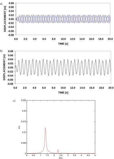
Figure 2.5.1: (a)Predicted absolute displacement histories of the liquid in a rigid container, (b) sloshing amplitude for the same case, (c) corresponding displacement frequency spectrum of sloshing liquid.

(57)

In Figure 2.5.1 (c) where the corresponding frequency spectrum of the sloshing history is

given, the fundamental sloshing frequency is suggested to be around 1.4 Hz, quite close

to the theoretical fundamental frequency of 1.34 Hz. Another small spectral peak is

apparent, around 2.3 Hz, indicating the second sloshing frequency.

A series of numerical trials was conducted to determine the most promising container

flexibility. The objective of the trials was to tune the container’s natural frequency to the

sloshing frequency. As mentioned before, two point masses of various magnitudes were

attached to obtain tuning at the middle point of the longer container walls. The presence

of significant energy transfer between the liquid and container is considered to be the sign

of appropriate tuning. Tuning generally produces a beat envelope in the displacement

history and two dominant spectral peaks in the corresponding frequency spectrum. This

beat should be apparent both in the displacement histories of the container and at the

liquid surface level.

The displacement history for the flexible container with 0 kg point mass is presented in

Figure 2.5.2 (a). The horizontal displacement histories of the container nodes are the top

and the bottom ones. The vertical displacement histories of the liquid surface nodes are

indicated with two middle lines, with smaller displacement magnitudes than those of the

container. Also, the container walls deflect substantially (an average of 0.075 m) after

filling the flexible container with water. As a result, the free surface oscillations take

place about a level lower that zero.

Liquid Sloshing in Containers with Flexibility