Inverse Method Applied to Adaptive Core Simulation

(1)

Abstract

ABDEL-KHALIK, HANY SAMY

.

Inverse Method Applied to Adaptive

Core Simulation

.

(Under the direction of Paul J. Turinsky)

.

The work presented in this thesis is a part of an ongoing research project

conducted to gain insight into the applicability of inverse methods to developing adaptive

simulation capabilities for core physics problems. Adaptive simulation is a simulation that

utilizes past and current reactor measurements of reactor observables (e.g. core reactivity

and incore instrumentation readings) to adapt the simulation in a meaningful way to

improve agreement with reactor observables. To perform such adaption, we utilize a

group of mathematical techniques which address the problem of given a current core

simulator model and the associated input data (e.g. cross-sections, thermal-hydraulic

parameters), how should the values of selected input data be adjusted to improve

agreement with observables without changing the core simulator model, (i.e. how can we

obtain the best agreement utilizing our current modeling capability). This is usually

referred to as an inverse problem, which is difficult to solve due to its ill-posedness nature.

Major advances have been made by mathematicians to overcome the ill-posedness nature

of such problems. The proposed project is of an exploratory nature serving to develop

expertise in this area, to which the nuclear power community has not participated to any

great extent over the last two decades since their earlier contribution during the design,

research and developments stages of a proto-typical fast breeder reactor. Exploratory

(2)

where little expertise is available, and to provide a basis on whether there is potential for

the proposed techniques to be useful and successful.

The current work addresses BWR core simulators since their prediction accuracy

is inferior to PWRs’, providing marginally acceptable agreement between measured and

predicted core attributes. This implies that BWRs could benefit from utilizing an adaptive

simulation tool. In the work done so far, a virtual approach has been utilized in which two

versions of a core simulator (i.e. FORMOSA-B) are utilized. The first one represents

actual plant data, and is referred to as the ‘virtual core’. In that version, the LPRM

readings and their associated instrumental noise have been simulated. The second one is

an altered version of the same core simulator, in which modeling and input data errors are

introduced to give rise to disagreement between the two versions of the core simulator,

and is referred to as the ‘design basis core simulator’. That disagreement is made to be of

the same magnitude as the actual disagreement which exists between plant data and

current core simulators in regard to LPRM readings and core criticality. The virtual core

observables at nominal conditions, including the noise component of the LPRM readings,

are then utilized to adapt the design basis core simulator. A larger set of virtual core

observables including those at nominal and various off-nominal core conditions, with and

without the noise signal, is then contrasted to those predicted by the ‘adapted design basis

core simulator’. Results indicate that the disagreement between the adapted design basis

core simulator and the virtual core can be decreased by an order of magnitude, indicating

the high fidelity and robustness of the adaptive techniques and that adaption can be

(3)

of this project. If successful in improving prediction fidelity when utilizing actual plant

data as the basis for adaption, this could lead to an increase in design margins and relaxing

of technical specifications, which will have a beneficial impact on reactor operation and

(4)

Inverse Method Applied to

Adaptive Core Simulation

by

Hany Samy Abdel-Khalik

A thesis submitted to the Graduate Faculty of

North Carolina State University

in partial fulfillment of the

requirements of the Degree of

Master of Science

Nuclear Engineering

Raleigh, North Carolina

2002

APPROVED BY:

(5)

ii

‘

Wisdom lies in Truth

’

(6)

iii

Biography

1

Hany S. Abdel-Khalik was born in Alexandria, Egypt on July 15th, 1978. He is the oldest of the five children of Samy I. Abdel-Khalik and Yousria M. Nourel-Deen. He

received his elementary education locally, graduating from Gamal Abdel-Naser High

School in 1995. He received his Bachelor of Science from Alexandria University in July

2000 from the department of Nuclear Engineering and he was the college valedictorian

that year. He was looking forward to continuing his graduate studies in the area of reactor

physics. Upon graduation, he had the wonderful opportunity to join the Electric Power

Research Center at North Carolina State University as a research assistant. Since the fall

of 2000 he has been working under the supervision of Dr. Paul J. Turinsky. He will

con-tinue his work on the project proposed in this thesis as a part of his PhD work. Hany holds

the ANS Allan F. Henry/Paul A. Greebler graduate scholarship, and is a recipient of the

ANS Reactor Physics Division best paper award at the Summer 2002 ANS national

meet-ing.

1. The author may be contacted at: Address: 1222 Burlington Labs,

North Carolina State University, P. O. Box 7909,

Raleigh, NC 27695-7909, USA.

(7)

iv

Acknowledgements

I would like to say thank you to many wonderful people in this very short space.

First, I thank my parents for their continuous support and strong will to provide for me the

best life possible. I also thank my siblings for their enormous love and self-sacrifice for

me. Dr. Mohamed E. Nagy has supported and encouraged me during my undergraduate

study, and to him I am indebted. I would like to thank my advisor Dr. Paul J. Turinsky for

giving me the chance to work on this wonderful project. His patience and support through

the first two years of my graduate study are very well appreciated. His innovative ideas

were among the main reason we won the ANS RPD best paper award. I have enjoyed the

insightful and intuitive discussions with Dr. Dmitriy Y. Anistratov and Dr. Carl D. Meyer.

I am very thankful to my uncle Dr. Said I. Abdel-Khalik; he has given me unconditional

support and care. His wife Sharon has given me invaluable advice. Finally, I thank Dr.

Youssef A. Shatilla for his recommendations and advice throughout my graduate and

(8)

v

List of Tables

Table 2.1: Isotopics treated in the core simulator model. . . . 21

Table 2.2: Selected set of adjusted microscopic cross-sections. . . . 21

(11)

viii

List of Figures

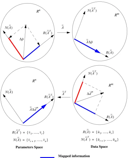
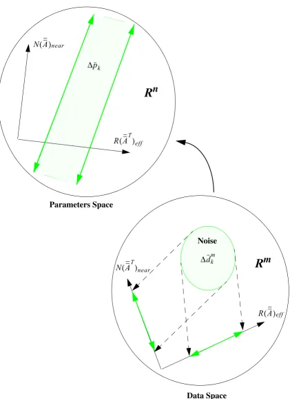
Figure 3.1: Mapping Information between Parameters and Data Spaces. . . 34

Figure 3.2: Notion of Best Approximation. . . 42

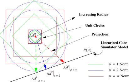
Figure 3.3: Projection of the Measured Observables onto the Linearized Core Model (Different Matrices). . . . 46

Figure 3.4: Inverse Mapping of Information in a ‘Discrete Ill-Posed System’. . . 53

Figure 3.5: Supplying A Priori Information about Model Parameters. . . . 56

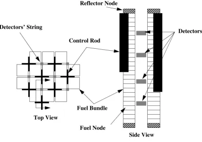
Figure 4.1: Detectors’ Layout. . . 61

Figure 4.2: Control Rod Pattern For Core Follow Data. . . . 71

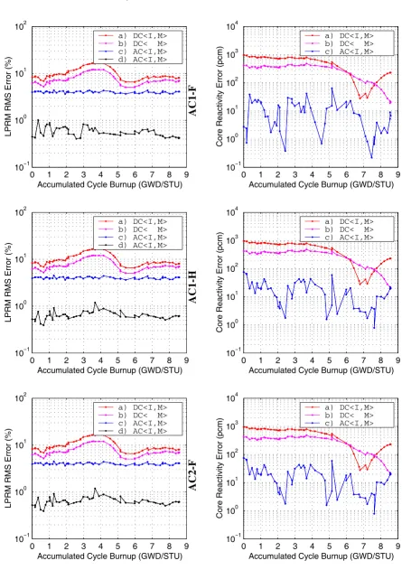
Figure 4.3: Detectors’ Signals Mismatch & Core Reactivity Error (Rated Conditions). 72 Figure 4.4: Simulated Core Follow Data at Rated Conditions, High Void and Low Void. . . 73

Figure 4.5: Detectors’ Signals Mismatch & Core Reactivity Error (High Void Fraction). . . . 74

Figure 4.6: Detectors’ Signals Mismatch & Core Reactivity Error (Low Void Fraction). . . 75

Figure 4.7: Detectors’ Signals Mismatch & Core Reactivity Errors (Different Criteria). . . 76

Figure 4.8: Detectors’ Signal Mismatch & Core Reactivity Errors.. . . 77

Figure 4.9: A Posteriori and A Priori Information About Model Parameters . . . 78

Figure 5.1: Road Map for Adaptive Core Simulation Project . . . 82

(12)

ix

Core Observables’.. . . 94

Figure B.2: Effect of Regularization on the Conditioning of the

Unconstrained Least-Squares Problem . . . 96

(13)

x

Nomenclature

Acronyms:

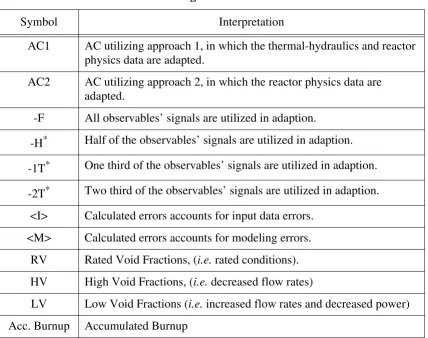
AC Adapted Design Basis Core Simulator.

BOC Beginning Of Cycle.

BWR Boiling Water Reactor.

CRH Control Rod History.

CRD Control RoD Insertion Branch Case.

DC Design Basis Core Simulator.

EOC End Of Cycle.

FP Fission Products Branch Case.

HFP Hot Full Power.

LPRM Local Power Range Monitors.

MWD Mega-Watt-Day

PWR Pressurized Water Reactor.

RMS Root Mean Square.

REF REFerence or Base Depletion Case.

STU Short-Tonnes-U, STU=1.1023113 MTU.

TIP Traveling Incore Probe.

TF Fuel Temperature Branch Case.

(14)

xi

Physical Symbols:

Void-quality concentration parameter.

Void-quality terminal velocity parameter.

Density of the vapor phase.

Density of the liquid phase.

Void fraction.

x Flow quality.

G Coolant mass flux.

Surface tension, microscopic cross-section or standard deviation.

Void-quality drift velocity parameter.

g Gravitational acceleration constant.

k_eff Core criticality eigenvalue.

Microscopic fast absorption cross-section.

Microscopic thermal absorption cross-section.

Microscopic fast fission cross-section.

Microscopic thermal fission cross-section.

Number of neutrons emitted per fission.

Energy emitted per fission.

C₀ k₃

ρ_g

α

σ

V_gj

σ_a₁

σ_a₂

σ_f₁

σ_f₂

v

(15)

xii

Variables’ Notations:

k Iterate number, (i.e. ).

m Measured Observables, (i.e. ).

c Calculated (e.g. predicted) Observables, (i.e. ).

Scalar quantity.

Vector quantity.

Matrix Operator.

p_k

dm

dc

*

(16)

CHAPTER 1: ADAPTIVE CORE SIMULATION 1

1. Adaptive Core Simulation

1.1. Importance to Advanced and Current Reactors

The accurate prediction of core behaviour is a fundamental requirement to the design

and operation of any nuclear reactor system. That is achieved through the utilization of high

fidelity core simulators. Core simulators can be utilized in either an on-line or off-line mode.

In the online mode, they provide support for the successful control and protection of the

reactor. Control systems are required to determine the optimum trajectory in moving the

reactor from the current state to a final desired state with all operational and safety limits

satisfied. Protection systems are required to be capable of determining current and near-term

reactor states for a range of reactor conditions to advise reactor operators, or to automatically

activate safety systems to help take the appropriate actions to avoid and/or mitigate any

accident scenarios. Off-line core simulators are also as important during the design as well as

operational phases of the plant to determine the optimum operating core conditions (i.e. fuel

loading pattern, control rod programming, etc.). They are also utilized to interpret

experimental results.

The quality of core simulators’ predictions will impact the reactor economy through

the introduction of design margins on the core design to ensure an operation, in which the

safety and operational limits are satisfied[1]. How tight or relaxed these margins are depends

on how accurate the predictions of core behaviour are. The uncertainties of core simulators’

calculations are thus very crucial to the determination of these margins. Large uncertainties

will result in diminishing core design freedom and hence adversely impact economics. On the

(17)

reactor economy such as reducing fuel and/or operating cost or even initial capital investment

for a new plant. By way of a few examples[2]: 1) By accurately calculating thermal limits, one

can reduce thermal margins, and be able to operate the reactor at higher power densities which

is economically more favorable (operating cost reduction). That translates into smaller sized

cores for new reactors (reduction in capital investment). 2) With more accurate calculations of

core reactivity for various states, one may be able to reduce the number of control rods

(reduction in capital investment), or reduce the U235 enrichment margin required in the fresh

fuel for the core to reach the desired cycle life at the desired rated power (reduction in fuel

cost).

High fidelity core simulators are hence essential components for any reactor system

during the design and/or the operational phases. To achieve, in the near term, this high level of

fidelity, dictated by economic, operational and safety considerations, will require high fidelity

and robust adaptive techniques[3]. Adaptive simulation techniques utilize past and current

reactor measurements of reactor observables to adapt the simulation in a meaningful way to

improve agreement with observable values. Fidelity denotes the ability of an adapted

simulator to accurately predict the measured observables. Robustness denotes the ability of

the adapted simulator to accurately predict measured core attributes which are not directly

observed, for example, the measured observables recorded at future times; and the observables

for core conditions that differ from those at which adaption is completed. Adaptive simulation

can also be useful in establishing a basis for deciding where future experimental efforts should

be focused to decrease core attributes’ uncertainties. That can be achieved by contrasting the

(18)

the impact their adjusted values will have on different core attributes, the costs associated with

uncertainties on these core attributes, and the costs of experiments to reduce core attributes’

uncertainties. The need for adaptive simulation is viewed to be greater for Generation IV

versus Generation II and III reactors, since limited applicable experience will be available for

Generation IV reactors. Adaptive simulation can also be used to effectively interpret

experimental results done in the course of developing Generation IV reactors, help determine

the major causes of discrepancies between predicted and measured values, and hence help

direct how the experimental program should be designed to reduce the uncertainties in the

evaluation of the important parameters.

1.2. Description of Core Simulators

The behaviour of a nuclear reactor core is governed by the neutron flux distribution in

space, energy and time. One of the central problems of core simulation models is to accurately

predict this distribution. The core simulator model consists of models for both reactor physics

and thermal-hydraulics, which is necessary to account for the non-linear feedback

mechanisms through cross-sections. Typically, reactor physics behavior is modeled

employing few-group neutron diffusion theory, hydraulics behaviour is modeled employing

some 1-D approximate form of the Navier-Stokes equations (e.g. drift flux model), and the

thermal behavior is modeled using some approximate thermal model (e.g. functionalizing fuel

temperature as a function of linear power density).

Input data to the core simulator are enormous and determined by the needs of the

models employed within. Note that we include in input data, the coefficients that appear in

(19)

thermal-hydraulic simulations require user input of core geometry as well as many empirical

parameters, such as local form loss coefficients and heat transfer coefficients. The input data

to the core simulator, in many cases, are determined using computer codes that model aspects

of the core physics in more detail than the core simulator models do, such as with the

determination of few-group homogenized cross-sections using lattice physics codes. So, in

general, the input data include any data directly passed to the core simulator or indirectly

through any preprocessor code.

Core observables include the readings of incore detectors (e.g. LPRMs and TIPs),

which are usually positioned throughout the core in between flow channels which do not have

control rods. Since core simulators are usually based on a steady state model and measured

observables are normally taken at steady state conditions, core reactivity could also serve as a

basis for adaption (e.g. at all times).

1.3. Sources of Simulation Errors

Core simulators introduce errors in the predicted core attributes, including core

observables, due to input data and computational (e.g. modeling) errors. Input data (e.g.

cross-sections and thermal-hydraulic parameters), whether they are experimentally measured or

theoretically calculated, contain uncertainties associated with their evaluation which are

described by standard deviation values reported as part of the data evaluation process.

Modeling errors occur due to different reasons: 1) The common practice in modeling is to

avoid sophistication by introducing approximations in the mathematical description to

simplify the treatment, that results in the introduction of errors in the calculations (i.e.

(20)

diffusion versus transport theory calculations for the whole core). 2) Inadequacies in the

mathematical model utilized for simulating the core (e.g. failure to present all aspects of the

physics governing the core behaviour). 3) Numerical solution techniques’ approximations (i.e.

spatial domain discretization).

The pre-processing codes also introduce errors into the core simulator’s input data,

hence into the core simulator’s predictions of core attributes. This follows since, just like the

core simulator, errors exist in the input data to the pre-processor codes, in the mathematical

models of the physics, and in the numerical solution techniques employed in these codes.

Computational methods and input data uncertainties have always been the sources of

the limitation of nuclear calculations. In some instances, the computational uncertainties

dominate the sources of discrepancies, however, over the last few decades computational

methods have reached a stage of maturity in their sophistication and applicability.

Computational power has also increased considerably enabling the solution of bigger

problems in relatively shorter computer execution times. With the current status of models’

sophistication and huge experience obtained from power plants’ operations, we believe that

more attention should be directed towards input data errors and show how these data can be

adjusted using measured plant data to effectively reduce the disagreement between the

measured (e.g. core observables) and predicted core attributes.

1.4. Adaptive Simulation Approach (Main Assumptions)

Adaptive simulation is a mathematical algorithm which deals with given a

mathematical model of certain physical phenomena and the associated input (model

(21)

input data, without adjusting the model, to reduce the disagreement between the measured and

predicted observables. The sources for the disagreement are either due to noise in the

measured output or simulation errors which, as described before, consist of modeling and

input data errors. Accordingly, it will be assumed that the dominant sources of errors in

predicted core attributes, including the core observables, originate due to errors in the input

data to the pre-processor codes and pre-processor codes’ independent input data to the core

simulator. That implies that input data will be adapted (e.g. adjusted) to improve the

agreement between predicted and measured observables, even though components of the

sources of disagreement are due to both input data and modeling errors. This assumption is

likely valid and also necessary in order to avoid the issue of simultaneous adaptation of the

core simulator’s models, since the combined adaptation problem of core simulator’s input data

and models is beyond current and foreseeable capabilities. However, a justification for that

assumption has to be investigated in this study by checking the fidelity and robustness of the

adaption.

1.5. Previous Development and Motivation for Adaptive Techniques

The art of data adjustment had been used extensively during the 1970s for fast

reactors’ experimentation. The data selected for adjustment were the cross-sections obtained

from differential experiments. The uncertainty level of the differential experiments’ evaluated

cross-sections did not meet the requirement for an accurate description of certain integral core

parameters, (i.e. breeding ratio[4] or k_eff eigenvalue). Uncertainty in the basic cross-section

data affects the uncertainty of the core integral parameters, which necessitate the introduction

(22)

allowances result in cost increases and reduction from optimum core performance. Integral

experiments’ results were used in conjunction with differential experiments to adjust

cross-sections, in a hope that this will reduce the important core parameters’ uncertainties[5] .

Integral experiments are typically critical assemblies operating at zero power, in which a

small-scale mock-up of the large-scale core is built to mimic the reactor core behaviour as

much as possible in regards to composition and geometry.

The idea for the proposed work of adaptive core simulation stems from these past

experiences[6]-[11]; but, with two major differences: The first is that instead of using small

scale experiments to simulate the operation of the real reactor, one can use the full-scale

experiment, (e.g. real core), as one’s integral experiment. This is advantageous when

considering the huge amount of core follow data from our operating experience with current

power plants. However, the interpretation of these data is much more complex than the

“clean” integral experiments, since the quality of the data in uneven. For integral experiments,

the quality of the data is considered to be the same, since there are no depletion effects and no

thermal-hydraulic feed-back effects. However for a power plant, these effects are present,

transient phenomena might be occurring at anytime yet a steady state core model is employed,

and instrumentation may not be properly calibrated or failed. Those are examples of such

difficulties one might encounter when interpreting plant data.

The second difference is in the mathematical formulation of the problem. The problem

at hand can be treated as an “inverse problem”, which is an extremely difficult problem.

However, over the last four decades, since the early papers by Tikhonov in 1963[12]-[13],

inverse methods have been extensively developed on a solid mathematical basis and have

(23)

advanced considerably using powerful inverse methods[14]. The nuclear power community

however has not participated to any great extent in these activities, in spite of their earlier

significant participation in the data adjustment area.

There are different issues and concerns that need to be analyzed when adjusting input

data. Reliability of the adjusted data denotes how well they will perform at different core

conditions and how consistent they are with the unadjusted data[15]. Uniqueness of the

adjustments denotes, would one obtain the same results if one starts from two different data

sets utilizing the same measured observables to adapt the core simulator? This type of analysis

can also help answer some other questions such as: 1) How well do the existing cross-section

or thermal-hydraulic data predict the core attributes of interest with the current modeling

capabilities? 2) How sensitive are certain core attributes to changes in the data, (i.e. use of an

alternative cross-section data set)? 3) How does one identify the sources/causes of

discrepancies between the core simulator’s predicted and measured core attributes?

Answering question (3) will provide direction to those areas of uncertainty where more

detailed experimental programs are required.

As a preable to the following discussion, note that the adaption approach we are

proposing to develop is for off-line application utilizing the observable data from many

different sources, including different reload cycles for the same nuclear power plant, different

nuclear power plants of the same type, and ultimately different types of nuclear power plants.

1.6. Current Practice

Very limited or no adaption is employed in current on-line core simulators, completed

(24)

between measurements and predictions are usually fitted using surface response

methodologies and are used to predict the discrepancy between future predictions and

measurements. Similar versions of this approach were utilized during the course of fast

reactors experiments, and are referred to as “bias factor methods”[16]. The “bias operator

method” is another mathematically elegant tool that has also been proposed in the past as a

method for adaption[17]-[20]. Neither of these methods will be utilized in our work, since we

believe they do not have a physical justification. In the proposed work, however, the

adjustments are done to the input data in a mathematically consistent way in which the physics

of the problem is satisfied. That is achieved by first limiting the input data adjustments by the

uncertainty information, sometimes propagated through the pre-processors’ codes to the core

simulator to preserve the proper pre-processor codes’ core physics behaviour. In doing so, the

proposed adjustments will be consistent with their known uncertainties. Second, the input data

adjustments will be propagated through the core model satisfying the physics described by the

core simulator. Physical justification is required when adapting core input data, since if the

physics of the core are not satisfied, one would not be able to predict core behaviour at

different operating conditions than those adapted to, defeating the whole purpose of the

adaption. Third, the uncertainties in the core observables will be accounted for during the

adaption, assuming that the input data adjustments are consistent with the quality of the

(25)

1.7. Inverse Problem

1.7.1 Definition and Areas of Application

From a mathematical point of view, the definitions of a direct problem and an inverse

problem are always ambiguous. This can be well illustrated by a frequently quoted statement

of J. B. Keller[22]: “We call two problems inverses of one another if the formulation of each

involves all or part of the solution of the other. Often, for historical reasons, one of the two

problems has been studied extensively for some time, while the other has never been studied

and is not so well understood. In such cases, the former is called the direct problem, while the

latter is the inverse problem.” So one of the two problems has been studied well, and the

physical model used to describe it is well understood and has been justified by experiments,

and usually is considered to be more fundamental than the other problem.

The notion of direct and inverse problems in engineering however can be described in

a more straightforward way[14],[21]. A forward problem can be defined to be the process in

which data are the output of some physical model, whose input are some physical parameters.

However, an inverse problem is one in which we are interested in estimating those parameters

on which the model depends, based on a prior knowledge of the data (the output of the

forward problem). From an experimental point of view, usually data are collected from any

system, to gain more information about the behaviour of that system, and if these data can be

described by a certain model we can predict the behaviour of that system under different

conditions. However, what we are interested in knowing is usually different from what we

measure, so, if we can use our mathematical model to extract information about what we want

(26)

unknowns) are the quantities that one is trying to estimate. The matter of how to choose these

parameters is usually problem dependent and quite often somewhat arbitrary. The inverse

problem is however less suited to provide the fundamental mathematics or physics of the

model itself. The main role of the theory is to infer numerical information about unknown

parameters of the model and not the type of the model itself; so a good idea of the applicable

forward model must be available in order to take advantage of the inverse theory. For

example, inverse theory can not suggest a new void-quality equation form to calculate the

amount of voiding in a BWR core; however it can determine the best values for the parameters

associated with a given void-quality evaluation form. Possible goals of an inverse analysis

might include 1) estimates of a set of model parameters, 2) estimates of the bounds on the

range or acceptable model parameters, 3) estimates of the formal uncertainties in the model

parameters, 4) sensitivity of the solution to noise (or small change) in the data, 5)

determination of the best set of data suited to estimate a certain set of model parameters, 6) the

adequacy of the fit between the predicted and observed data, and 7) directions to decide

whether a more sophisticated model will be significantly better than a more simple one or not.

All these goals emphasize that inverse theory is not just used to determine the optimum values

for model parameters but also provides different criteria by which the quality of those

estimated parameters can be judged. It is to be noted, however, that a solution to an inverse

problem might contain not a “single” answer like a forward problem, so one of the parts of the

inverse analysis is the ability to determine which answer is reasonable, valid, and acceptable.

Inverse theory has found many applications in many different branches of physical

(27)

and earthquake location determination, (c) satellite navigation, (d) molecular structure by

x-ray diffraction, and (e) medical tomography.

1.7.2 Mathematical Description

Inverse theory has been developed over the past four decades by scientists and

mathematicians having various backgrounds. This has resulted in presenting the theory in

many different ways[21], tending to superficially look very different in spite of the strong and

fundamental similarities that exist between them. Inverse theory can be derived from (1) pure

statistical concepts, (i.e. Bayesian decision analysis, and information content concepts), or

from more (2) deterministic ways which avoids mentioning terms like probability distribution

and prefer terms like inverse transformation, (i.e. minimum variance approaches). Inverse

theory can also be classified according to the type of both the model parameters and the

observed data by whether they are continuous functions or discrete values. The problem we

are interested in is a discrete-discrete problem, which means that both the data and the

parameter space are discrete or finite dimensional spaces. This will make our mathematical

analysis much easier than the general inverse theory. The reasons behind the finite

dimensionality of our problem is that our observables are instrument readings, and the

parameters we are looking for are ones associated with the thermal-hydraulic and reactor

physics model, (e.g. thermal property constants and cross-sections).

A discrete inverse problem is much simpler than the continuous one, since the

mathematical vehicle needed for the discrete case is linear algebra, and ideas like vector

spaces and matrix representation of linear transformations are sufficient to fully describe the

(28)

techniques by vector space methods[23],[24]. For the continuous case, the problem gets much

more complicated and more abstract elements from the theory of functional analysis are

needed to describe the problem. Functional analysis abstracts our intuition about geometry of

ordinary vector spaces by merging linear algebra and analysis. The functional analysis

approach reveals itself to be tremendously more powerful and elegant than the linear algebra

approach. That leads some readers to hope that these elegant tools might help solve much

more complicated problems beyond the reach of the simple mathematical analysis provided by

linear algebra. Unfortunately, realization of such hopes is rarely encountered in practice. The

primary role of functional analysis is to unify and abstract our simple ideas about vector

spaces in a more mathematical and rigorous fashion.

In general, inverse theory can be described in a continuous form and then the special

discretization for the specific problem of interest can subsequently be introduced[25],[26].

However, since the problem of interest is a discrete one, the fully mathematical rigorous

treatment of the continuous inverse problem will be considered to be beyond the scope of this

work, and only the discrete inverse problem will be presented.

Inverse problems can be either under or over-determined. For the core simulator[3],

the problem is under-determined in that there are many more input data items that can be

adjusted than there are observables. Parametrization of the system is one way to recast the

problem from an under to over-determined one. Parametrization, within the context of our

application, is the process of characterizing core simulator data in terms of a minimal set of

parameters, which we shall refer to as core parameters. Care is required in the selection of

those parameters since improper choices made will be reflected in poorer fidelity and/or

(29)

approach to determine the unknown core parameters, so as to minimize the differences in the

predicted and measured values of the observables. The weights can be selected to reflect the

uncertainties in both the observables and input data. This least squares problem will likely be

ill-posed or at least ill-conditioned.

1.7.3 Ill-Posed Problems

A problem is said to be ill-posed if it is not well-posed. According to the french

mathematician Jacques Hadamard[27], for a problem to be well-posed, the following three

conditions, within the context of the current application, must exist: 1) There is a solution for

the core parameters. 2) The solution for the core parameters is unique. 3) The values of core

parameters change smoothly with smooth changes in the values of the observables. Item (1) or

Item (2) if not satisfied is obviously troublesome in that either no or a non-unique solution for

the core parameters exists. Item (3) if not satisfied is troublesome since it implies that the

values of core parameters are highly sensitive to the values of observables. Given that

observables contain experimental errors, one cannot tolerate the high sensitivity associated

with Item (3). This item also has implications with regard to robustness of adaptation. The

mathematical distinction between a well- and an ill-posed problem is very clear. However, in

practice, when considering the discretization of the problem and the associated errors (noise)

in the measured observables, that distinction reveals itself to be less apparent. In some cases,

one cannot obtain an accurate, unique solution for a well-posed problem due to the finite

precision of the computations, forcing us to treat such problems as ill-posed. Further details

(30)

1.7.4 Regularization of Ill-Posed Problems

In Hadamard’s opinion, an ill-posed problem does not have a physical meaning.

However, it turns out that an ill-posed problem can be extended to a well-posed one. That

extension is usually obtained by recognizing that the information supplied by the observables

about model parameters is not sufficient to give rise to a well-posed problem. Regularization

refers to the mathematical methods utilized to incorporate extra information about model

parameters necessary to recast an ill-posed problem into a well-posed one. An ill-posed

problem is regularized by either altering the mathematical model of the physical processes or

by restricting the space of the solutions allowed. The first technique of altering the

mathematical model will not be addressed in this study, since the intention is to enhance the

current models’ prediction accuracies without changing these models. Functionalization is one

manner of restricting the space of the solutions allowed to address ill-posedness, but many

times, is not adequate. Therefore, additional constraints may need to be applied to restrict the

solution space. There are many manners of performing regularization, ranging from those

based upon “energy” minimization approaches to those based upon Bayesian decision

analysis. A solid mathematical basis has been developed for unifying various regularization

approaches and understanding under what conditions regularization is effective[25]-[29].

Effective regularization methods factor in uncertainties in observables (measurements), a

priori and a posteriori knowledge of uncertainties in parameters to be adjusted, and robustness

of adaptation. The a priori and a posteriori information are the best available information

(31)

1.8. Scope of Work

Our target is to reduce the disagreement between actual plant data and core simulators’

predictions of core attributes, however, at the current stage of project development, a virtual

approach is utilized to develop insight into the proposed adaptive techniques. Chapter 2

discusses this approach in details and briefly discusses the core simulator we employed in the

study (e.g. FORMOSA-B1). The selected core simulator’s parameterization is also presented.

Chapter 3 is devoted to introducing the discretized version of the inverse theory which has

been employed in our work. In chapter 4, some selected test cases associated with the virtual

approach are investigated to assess the adaptive techniques. Chapter 5 presents our

recommendations for further development in the area of adaptive core simulation.

(32)

CHAPTER 2: VIRTUAL APPROACH 17

2. Virtual Approach

2.1. Description of the Virtual Approach

As mentioned in the introductory chapter, this thesis presents elementary work

undertaken as a part of an exploratory project to develop adaptive simulation techniques

which will enhance the agreement between measured and predicted core attributes, including

core observables. Therefore, the main target in this work is to contrast the predictions of the

adapted core simulator to actual plant data, in an effort to assess and validate the proposed

techniques. However, since the project is still in its exploratory stages, a virtual approach will

be adopted for assessing the fidelity and robustness of the techniques. In this approach, the

actual plant data will be produced by an existing version of a core simulator, that will be

referred to as a virtual core, denoted by VC. Since the plant data consists of the readings of

incore detectors (i.e. LPRMs and TIPs signals), the virtual core will be used to simulate those

detectors’ responses, and in doing so the noise on those responses will also be simulated by

perturbing their signals from their simulated values by sampling them from a Gaussian

distribution of standard deviation of 0.04 of the average relative detectors’ response which is a

representative value of the actual instruments’ noise signals. Since adaptive techniques are

supposed to address and adjust for the different sources of prediction errors, an altered version

of the same core simulator will be used after deliberately introducing two major sources of

errors, specifically, in its modeling and in its input data. This version of the core simulator will

be referred to as the design basis core simulator, denoted by DC. The size of the introduced

errors in the DC will be chosen so as to create discrepancies between the predictions of the VC

(33)

the actual discrepancies found between real plant data and existing core simulators’

predictions. A representative value for the core reactivity prediction error is around

pcm, and the RMS error for relative detectors’ signals is about 6%. The

FORMOSA-B core simulator[30]-[32] was utilized to both generate the values of the

experimental observables and as the core simulator to be adapted.

2.2. Advantages of Virtual Approach Utilization

In contrast to utilizing operating power plant observables, the virtual core approach

has several attractive properties in regard to developing an adaptive core simulator

methodology, such as the following: 1) Knowing exactly the sources of errors in the method,

input data and observables. 2) Providing a basis to study the effects of the parametrization of

core simulator model on the fidelity and/or robustness of the adaptive simulator. 3) Having not

to contend with the complexities of core simulator and pre-processor introduced methods’

errors. 4) Being able to evaluate the prediction accuracies of non-observables (i.e. thermal

margins) obtained from pre- and post-adaptation.

2.3. Core Parameterization

This section presents a brief description of the core models and input data which were

perturbed and/or adapted in the virtual approach. In practice, as mentioned in the introductory

chapter, the input data to be adapted will be first functionalized in terms of core parameters to

render an over-determined problem. A detailed discussion of the parameterization selected in

(34)

2.3.1 Thermal-Hydraulics Core Parameterization (Simulation of Modeling Errors)

The first major source of prediction errors included in the virtual approach is the one

due to modeling errors. The modeling of voids in a BWR core has a large impact on the

prediction of different core attributes. Predictions of power distribution and reactivity are

known to be very sensitive to the moderator void (density) distribution. That necessitates the

utilization of a reasonably high fidelity void-quality correlation in order to predict core

attributes to a reasonable degree. Based on that fact, the void-quality correlation was elected

to be perturbed in the DC. The void-quality1 relationship is given by the form first identified

by Zuber-Findlay[33],

, (2-1)

where

. (2-2)

The DC utilized the Zuber-Findlay void-quality correlation in which two variables, the

concentration parameter (C₀) and terminal velocity parameter (k₃), were assumed spatially

independent throughout the core and given by their best known values,

(2-3)

Both variables were elected as input data to be adapted according to the relationship:

(2-4)

1. Refer to Moore’s PhD thesis for more details[32].

α x C₀ x ρ_ρg

l

---(1–x)

+ ρgVgj

G

---+

 

 

⁄ =

V_gj k3 (ρl–ρg) ρ_l2 ---σg

1 4⁄

=

C₀ = 1.13 ; k₃ = 1.41

(35)

where the factors represent the selected thermal-hydraulics core parameters

which are to be determined by the adaptive techniques, and are the adapted

void-quality constants utilized in the adapted design basis core simulator, denoted by AC, to

calculate the void fraction. The virtual core utilized the Lellouche-Zolotar EPRI

methodology[34] to determine C₀ and k₃, which can be thought of as using spatially

dependent C₀ and k₃. The purpose of this difference in functionalizing the void-quality

relationship between the VC and the DC is to investigate how well the adaptive technique will

perform when the functionalization of the data is not consistent with reality, and how an

adaptive technique can account separately for the combined sources of errors due to

inconsistent modeling and input data errors.

2.3.2 Reactor Physics Core Parameterization

The second major source of errors included in the virtual approach is the one due to

input data errors (e.g. hydraulics and reactor physics input data). The

thermal-hydraulics data in the current study consists of only the C₀ and k₃, coefficients of the

Zuber-Findlay void-quality correlation. The reactor physics input data consists of all types of

few-group homogenized fast and thermal microscopic cross-sections of all nuclides, included

explicitly or implicitly in the microscopic depletion model of the utilized core simulator (e.g.

FORMOSA-B). Table 2.1 presents the set ( ) of all the fuel, burnable poison and pseudo

isotopes considered in the core simulator model, and Table 2.2 presents the corresponding

microscopic cross-section set ( ) selected for adjustment according to each nuclide’s

fc0

and fk3

C˜0 and k˜3

ζ

(36)

classification. The cross-section representation developed in FORMOSA-B[35] requires that a

number of ‘cases’ be generated at the lattice physics level. Base micro and/or macroscopic

cross-sections are obtained from a lattice physics unit assembly depletion at the nominal hot

full power (HFP) average core conditions at different vapor void fractions. From these base

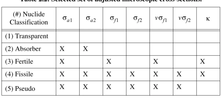
depletions, branch cases are performed to capture the instantaneous effects of perturbing (#) Nuclide Classification

(X) Denotes a cross-section type that is adjusted.

Table 2.1: Isotopics treated in the core simulator model.

Treatment in Depletion

Model Element Element-Isotope (Classification)

Explicit Actinides

U-234(1), U-235(4), U-236(4), Np-239(1), U-238(3) Pu-239(4), Pu-240(4), Pu-241(4), Pu-242(4), Am-243(4)

Burnable

poisons Gd-154(2), Gd-155(2), Gd-156(2), Gd-157(2), Gd-158(2)

Implicit

Pseudo isotope

Represents background macroscopic cross-section(5) for ele-ments not directly included in the depletion model.

Table 2.2: Selected set of adjusted microscopic cross-sections.

(#) Nuclide Classification

(1) Transparent

(2) Absorber X X

(3) Fertile X X X X

(4) Fissile X X X X X X X

(5) Pseudo X X X X X X

(37)

different core conditions like fuel temperature, coolant void, and control rod insertion. This

requires that different branch case calculations be made at various exposures within the set of

the reference depletion exposures like fuel temperature decrease or increase, instantaneous

void fraction correction, and control rod insertion at HFP. The data read from these branch

cases along with the base depletions are used to model the local thermal-hydraulic feedback

and transient fission product feedback effects. The cross-section is constructed as the

summation of a reference and a set of correction terms given by:

, (2-5)

where the reference term is the first term on the R.H.S. and is a function of fuel exposure, and

instantaneous and history void fractions. The rest of the terms can be considered as correction

terms, the first one is a function of control rod history, second one represents fuel temperature

Doppler broadening effect, third one is due to fission products poisoning, and the last one

represents the instantaneous control rod insertion effect. The reference and the correction

terms are constructed using piece-wise cubic splines and quadratic fitting polynomials. A

reference or correction term k of a cross-section type j for a nuclide n in a fuel color c is given

by:

, (2-6)

where is a state variable describing the dependence of the specific cross-section reference or

correction term on different core conditions (i.e. fuel temperature, void fraction, etc.),

{ } are the polynomial coefficients calculated based on the lattice physics data, and are Σ = ΣREF+ΣCRH+ΣTF+ΣFP+ΣCRD

Σn j k c, , , (Bu) dn j k c_i, , , (Bu) y_i( )x

i=1

I

∑

=

x

(38)

functionalized in terms of the fuel exposure, Bu, and { } are polynomial functions. The base

or correction terms are adapted according to the relation:

(2-7)

where the factors are functionalized in terms of fuel exposure according to the

following relation:

(2-8)

with the factors representing the reactor physics core parameters which

are to be determined by the adaptive techniques, and is a scaling factor with exposure

units.

2.4. Simulation of Input Data Errors

The direct approach to simulate input data errors would be one in which each input

data from the set studied (e.g. and the lattice physics few-group homogenized

cross-sections library) is randomly selected from a normalized Gaussian distribution whose standard

deviation corresponds to the relative uncertainty for that specific input data. One can then

assume that the perturbed values are our current best knowledge of these data.

The uncertainty information is not directly available though, and to obtain it, one

would need to propagate the uncertainty information starting from an energy point-wise or

resonance parameters presentation like ENDF/B to a few group, spatially homogenized

y_i

Σ˜n j k c, , , (Bu) f_in j k c, , , (Bu)d_in j k c, , , (Bu) y_i( )x

i=1

I

∑

=

f_in j k c, , ,

fn j k c_i, , , (Bu) fn j k c_i_,, , ,₁ (1–f_in j k c_,, , ,₂ )Bu

Bu˜

---+

=

f_in j k c_,, , ,₁ ,f_in j k c_,, , ,₂

{ }

Bu˜

(39)

presentation provided by most lattice physics codes. This is not a trivial task to do and requires

substantial calculational efforts. For that reason and for the sake of an exploratory

investigation, a cruder approach will be utilized. In this approach, the input data are

considered to be fully characterized by the selected core parameters1 (e.g. , and

{ }). To simulate input data errors in this cruder approach, each of the core

parameters will be randomly selected from a normalized Gaussian distribution whose standard

deviation is assumed now to be the same for all core parameters. A constant standard

deviation (1%) is selected, so as to give rise to discrepancies between the predictions (LPRMs

readings and core reactivity) of the VC and DC which are representative of the actual

magnitude of such discrepancies found between real plant data and existing core simulators.

After perturbing the core parameters in this fashion, the original input data can be represented

by:

(2-9)

where now the perturbed core parameters (e.g. , and { }) will be

assumed to constitute our best knowledge (e.g. the a priori information) about the input data to

simulate input data errors in the virtual approach.

Note that each of the reference and corrections terms are functionalized in terms of the

void fraction (through ), so when one is adapting the void-quality parameters and the

polynomial coefficients as well, one is explicitly correcting separately for the void-quality

1. Note that the unperturbed values for the selected core parameters are all equal to 1.0.

fc0

fk3 ,

f_in j k c_,, , ,₁ ,f_in j k c_,, , ,₂

Cˆ₀ ˆfc0

C₀; kˆ₃ ˆfk3

k₃; dˆ_in j k c, , , fˆn j k c_i_,, , ,₁ (1–ˆf_in j k c_,, , ,₂ )Bu

Bu˜

---+

 

 _d

i n j k c, , ,

= = =

f

ˆc0

f

ˆk3

, fˆin j k c,, , ,1 ,fˆin j k c,, , ,2

(40)

modeling error and the input data errors (to a first-order approximation). Consider a small

perturbation in all the core parameters, the resulting perturbation in the cross-section is given

by,

where to a first order approximation, is given by,

,

and hence,

.

However, if one is not adapting the void-quality correlation, the adjusted reactor physics core

parameters { } will be accounting both for input data and modeling errors as well, but

only for those specific core conditions at which the adaption was completed (e.g. certain core

average void fraction). That could lead to a less robust adaption when trying to predict core

behaviour at different core conditions. This issue will be investigated in the study to show how

powerful the adaption can be utilized to separately adjust for the different sources of

prediction errors and give insight to situations when adaption is performed on the wrong input

parameters.

Σn j k c, , , +∆Σn j k c, , , (f_in j k c, , , +∆f_in j k c, , , )dn j k c_i, , , (y_i( ) ∆x + y_i( )x ) i=1

I

∑

=

∆y_i( )x

fc0 ∂

∂ _y

i( )∆x f c0

fk3 ∂

∂ _y i( )∆x f

k3 +

=

∆Σn j k c, , , f_in j k c, , , d_in j k c, , , fc0 ∂

∂ _y i( )∆x f

c0 =

f_in j k c, , , d_in j k c, , , fk3 ∂

∂ _y i( )∆x f

k₃

+

y_i( )x d_in j k c, , , ∆f_in j k c, , ,

i=1

I

∑

+

(41)

To simplify the adaption, dependencies of the reactor physics core parameters

{ } will be restricted to nuclides (n) and reactions types (j) with dependencies on

correction terms (k), fuel colors (c) and fitting polynomials (i) dropped. In reality, correction

terms are expected to be dependent upon branch cases and fuel color, since the unit lattice flux

energy and spatial shapes are dependent upon these attributes. Hence, the few-group

homogenized cross-sections errors are also dependent on different branch cases and fuel

colors. As this project moves forward, more sophistication will be introduced. Even with this

simplification, a total of 108 core parameters were free to adapt.

(42)

CHAPTER 3: DISCRETE INVERSE THEORY 27

3. Discrete Inverse Theory

3.1. Objective

The applications of the inverse theory are diverse and include many areas of science;

however, the emphasis in this work will mainly be on core physics problems. Most of the

introduced nomenclature, notations and examples are selected specifically to serve our

application. Minor modifications are required to generalize the methods and discussion to

other areas of interest. The subject of the generalized inverse theory is very mathematical in

nature and most of the ideas need extensive rigor and mathematical abstraction to be

comprehensively and concisely presented. The mathematical tools necessary for our work will

be presented; however, the discussion will not be highly mathematical and is not intended to

be neither comprehensive nor complete. The intent is to present the more intuitive ideas

behind the utilization of these tools rather than the more abstract mathematical rigor. We

choose to do this for three reasons: 1) The more extensive and rigorous treatment of the

subject is already well established in the literature and stands on a very firm basis[25]-[26], so

it would be redundant to reproduce these mathematical results in this work even in part. 2) We

believe in a more realistic illustration of the abstract mathematical ideas, and that heavy

abstraction serves to generalize rather than to develop our understanding about certain

phenomena. Hopes for solving more complicated problems by utilizing the abstract and more

complicated version of the theory are rarely encountered in practice. 3) Our work is intended

primarily for engineers rather than for mathematicians. For these reasons, the concepts are

emphasized more than the technicalities in order to avoid confusion. Narrative discussions and

(43)

However, to avoid a speculatory type discussion, an extensive bibliography will be referenced

to support the discussion whenever necessary.

The discussion will be confined to the discrete linear inverse theory. This implies that,

in order to apply the theory, we will need to linearize the core simulator model and employ an

iterative strategy to search for the optimum core parameters’ values. Almost every problem in

discrete inverse theory can be recast into an optimization problem, where a function must be

minimized subject to various constraints. Optimization techniques for discrete problems can

best be described by vector space methods since the whole theory can then be derived from a

few simple, intuitive and geometric relations. A large number of problems can be analyzed

utilizing those simple relations. The texts by Luenberger[30] and Dorny[24] present

comprehensive and insightful approaches to optimization methods using vector space

methods.

3.2. Definitions

In this section an informal survey of some of the essential definitions, within the

context of our application, is introduced[21],[36].

3.2.1 Parameter Space

The parameter space is defined as the vector space whose elements represent the set of

core parameters we are trying to estimate. Let n be the number of such parameters, and a

vector of dimension n which lies in the parameters space ( ) and denotes the core

parameters.

∆p

(44)

3.2.2 Data (Observables) Space

The data space is defined as the vector space whose elements are the values of the core

observables. Let m be the number of such observables, and let be vectors of

dimension m which lie in the data space ( ) and denote the measured and

predicted (calculated) observables, respectively1.

3.2.3 Linear Transformation

A function that associates with every point in the parameters’ space a

point in the data space is said to be linear if it satisfies the following condition,

(3-10)

where . The action of a linear function is referred to as a linear transformation

which can be characterized by a matrix operator . One can visualize the operation of such a

transformation from different view points. Meyer[37] presents one such rigorous and

insightful discussion of the subject. Linear transformation is the process in which each point

in the parameters space is mapped to a unique point in the observables

space, this unique correspondence determined by the matrix , where and can be

described by,

1. The notations are enforced here to avoid introducing extra notations later in the discussion since the linearization of the core simulator model will require the utilization of these notations. nota-tion denotes the difference between the variable of interest (e.g. core parameters or observables) and some reference value.

∆dm and ∆dc

Rm ∆dm,∆dc∈Rm

∆

Ψ ∆p∈Rn

∆dc∈Rm

Ψ α( ₁∆p₁+α₂∆p₂) = α₁Ψ ∆( p₁) α+ ₂Ψ ∆( p₂) for all scalars α₁ and α₂

∆p₁,∆p₂∈Rn

A

∆p∈Rn ∆dc∈Rm

(45)

. (3-11)

3.2.4 SVD Decomposition

To gain more insight into the anatomy of such a transformation, the SVD

decomposition of the matrix is introduced[38]-[40]. Any matrix has an

orthogonal decomposition such that,

, (3-12)

where and are orthogonal matrices (their columns constitute orthonormal bases for the

spaces and , respectively). The columns of and are called the left and right

singular vectors of the matrix . is a diagonal matrix containing the singular values of the

matrix . These matrices are given by,

,

where

,

, ∆dc = A∆p

A A∈Rm n×

A = USVT

U V

Rm Rn U V

A S

A

Um m× = u₁ u₂ ... u_m , Vn n× = v₁ v₂ ... v_n

Sm n×

σ₁ σ₂

.. σ_r

0 ..

0 .. 0 =

u_iTu_j= δ_ij for 1≤i j m, ≤

Inverse Method Applied to Adaptive Core Simulation

Abstract

.

Inverse Method Applied to Adaptive

Core Simulation

.

.

Inverse Method Applied to

Adaptive Core Simulation

Hany Samy Abdel-Khalik

A thesis submitted to the Graduate Faculty of

North Carolina State University

in partial fulfillment of the

requirements of the Degree of

Master of Science

Nuclear Engineering

Raleigh, North Carolina

2002

APPROVED BY:

‘

Wisdom lies in Truth

’

Biography

1

Acknowledgements

Table of Contents

List of Tables

List of Figures

Nomenclature

Acronyms:

Physical Symbols:

Variables’ Notations:

1. Adaptive Core Simulation

1.1. Importance to Advanced and Current Reactors

1.2. Description of Core Simulators

1.3. Sources of Simulation Errors

1.4. Adaptive Simulation Approach (Main Assumptions)

1.5. Previous Development and Motivation for Adaptive Techniques

1.6. Current Practice

1.7. Inverse Problem

1.8. Scope of Work

2. Virtual Approach

2.1. Description of the Virtual Approach

2.2. Advantages of Virtual Approach Utilization

2.3. Core Parameterization

∑

2.4. Simulation of Input Data Errors

∑

∑

∑

3. Discrete Inverse Theory

3.1. Objective

3.2. Definitions