Maximizing the Reliability of Genomic Selection by Optimizing the Calibration Set of Reference Individuals: Comparison of Methods in Two Diverse Groups of Maize Inbreds (Zea mays L.)

(1)

Maximizing the Reliability of Genomic Selection

by Optimizing the Calibration Set of Reference

Individuals: Comparison of Methods in Two

Diverse Groups of Maize Inbreds (

Zea mays

L.)

R. Rincent,*,†,‡,§_{D. Laloë,** S. Nicolas,* T. Altmann,}††_{D. Brunel,}‡‡_{P. Revilla,}§§_{V. M. Rodríguez,}§§ J. Moreno-Gonzalez,*** A. Melchinger,†††_{E. Bauer,}‡‡‡_{C-C. Schoen,}‡‡‡_{N. Meyer,}‡_{C. Giauffret,}§§§ C. Bauland,* P. Jamin,* J. Laborde,**** H. Monod,††††_{P. Flament,}§_{A. Charcosset,*},1_{and L. Moreau*} *Unité Mixte de Recherche (UMR) de Génétique Végétale, Institut National de la Recherche Agronomique (INRA), Université Paris-Sud, Centre National de la Recherche Scientiﬁque (CNRS), 91190 Gif-sur-Yvette, France,†BIOGEMMA, Genetics and Genomics in Cereals, 63720 Chappes, France,‡KWS Saat AG, Grimsehlstr 31, 37555 Einbeck, Germany,§Limagrain, site d’ULICE, av G. Gershwin, BP173, 63204 Riom Cedex, France, **UMR 1313 de Génétique Animale et Biologie Intégrative, INRA, Domaine de Vilvert, 78352 Jouy-en-Josas, France,††Max-Planck Institute for Molecular Plant Physiology, 14476 Potsdam-Golm, Germany, and Leibniz-Institute of Plant Genetics and Crop Plant Research (IPK), 06466 Gatersleben, Germany,‡‡Unité de Recherche (UR), 1279 Etude du Polymorphisme des Génomes Végétaux, INRA, Commisariat à l’Energie Atomique (CEA) Institut de Génomique, Centre National de Génotypage, 91057 Evry, France,§§Misión Biológica de Galicia, Spanish National Research Council (CSIC), 36080 Pontevedra, Spain, ***Centro de Investigaciones Agrarias de Mabegondo, 15080 La Coruna, Spain,†††Institute of Plant Breeding, Seed Science, and Population Genetics, University of Hohenheim, 70599, Stuttgart, Germany,‡‡‡Department of Plant Breeding, Technische Universität München, 85354 Freising, Germany,§§§INRA/Université des Sciences et Technologies de Lille, UMR1281, Stress Abiotiques et Différenciation des Végétaux Cultivés, 80203 Péronne Cedex, France, ****INRA, Stn Expt Mais, 40590 St Martin De Hinx, France, and††††INRA, Unité de Mathématique et Informatique Appliquées, UR 341, 78352 Jouy-en-Josas, France

ABSTRACTGenomic selection refers to the use of genotypic information for predicting breeding values of selection candidates. A prediction formula is calibrated with the genotypes and phenotypes of reference individuals constituting the calibration set. The size and the composition of this set are essential parameters affecting the prediction reliabilities. The objective of this study was to maximize reliabilities by optimizing the calibration set. Different criteria based on the diversity or on the prediction error variance (PEV) derived from the realized additive relationship matrix–best linear unbiased predictions model (RA–BLUP) were used to select the reference individuals. For the latter, we considered the mean of the PEV of the contrasts between each selection candidate and the mean of the population (PEVmean) and the mean of the expected reliabilities of the same contrasts (CDmean). These criteria were tested with phenotypic data collected on two diversity panels of maize (Zea maysL.) genotyped with a 50k SNPs array. In the two panels, samples chosen based on CDmean gave higher reliabilities than random samples for various calibration set sizes. CDmean also appeared superior to PEVmean, which can be explained by the fact that it takes into account the reduction of variance due to the relatedness between individuals. Selected samples were close to optimality for a wide range of trait heritabilities, which suggests that the strategy presented here can efﬁciently sample subsets in panels of inbred lines. A script to optimize reference samples based on CDmean is available on request.

A

MONG the different methods that use molecular

mar-kers for selection, genomic selection (GS) has received considerable attention in the last decade. The objective of this approach is to predict the breeding values of candidates based on their molecular marker genotypes. A prediction formula is developed using the genotypes and phenotypes of reference individuals forming a calibration set (Meuwissen Copyright © 2012 by the Genetics Society of America

doi: 10.1534/genetics.112.141473

Manuscript received May 1, 2012; accepted for publication July 19, 2012

Supporting information is available online athttp://www.genetics.org/lookup/suppl/ doi:10.1534/genetics.112.141473/-/DC1.

1_{Corresponding author: UMR de Génétique Végétale, INRA, Univ Paris-Sud, CNRS,} AgroParisTech, Ferme du Moulon, F-91190, Gif-sur-Yvette, France. E-mail: alain. [email protected]

(2)

et al. 2001). The GS formula potentially includes all the

marker effects, without preselection based on a signiﬁcance

threshold. If the marker density is sufﬁcient, this permits the model to capture an important part of the genetic variance

(Yanget al.2010). Compared to traditional marker-assisted

selection (MAS), the efﬁciency of which is limited by

the power of marker-trait association tests, GS is expected

to be more efﬁcient, especially for highly polygenic traits

(Bernardo and Yu 2007). GS wasﬁrst used in animal

breed-ing, particularly dairy cattle, and its use clearly improved

the selection efﬁciency (Hayes et al.2009a). It is now also

widely studied by plant breeders, and interesting results

were obtained (Jannink et al.2010; Crossa et al. 2010;

Albrecht et al.2011).

Powerful statistical tools and relevant data sets (geno-types and pheno(geno-types to train the prediction model) are key

factors for the predictive efﬁciency. There are two ways to

use the genotypic data in genomic selection. Theﬁrst way is

to estimate the marker effects in the calibration set and then to predict the breeding values of the selection candidates by multiplying their genotypes by the marker effects. This approach is used, for example, in the mixed model called

random regression–best linear unbiased predictions (RR–

BLUP; Whittaker et al. 2000; Meuwissen et al.2001). The

second approach is to use the marker genotypes to estimate a relationship matrix between phenotyped individuals of the reference population and nonphenotyped individuals, can-didates to selection. This relationship matrix can then be used to estimate a variance/covariance matrix between the

genetic values in a mixed model called RA–BLUP (RA for

realized additive relationship matrix; Zhonget al.2009), or

G–BLUP. It has been proven that RR and RA–BLUP are

sta-tistically equivalent under conditions presented by Habier et al.(2007), Goddard (2009), and Hayeset al.(2009b).

The implementation of genomic selection is facilitated by recent advances in genotyping. We now have access to geno-typing arrays, which provide genotypes of very good quality at low cost. The costs of sequencing are also decreasing and it is, or will soon become, possible to genotype the genetic

material by sequencing (Huang et al.2009; Metzker 2009;

Elshireet al.2011). In plant breeding, large collections of in-dividuals are usually available to the breeder, corresponding to germplasm released by public institutes, private germplasm released at the end of their protection by patent (PVP), and individuals that have been used as parents of the current breeding program. All this material can be easily genotyped and potentially used to create the calibration set. Conversely, although there have been very important advances in the automatization of phenotyping, it is still very expensive to obtain relevant phenotypes with a high heritability for a large set of individuals. In addition, multi-environment trials are needed to test individuals under different conditions and es-timate the genotype x environment interactions (GEI). As a result, it is now clearly admitted that the collection of phe-notypic data relevant in terms of traits and environmental conditions with respect to the breeding objectives is the most

limiting factor for running genomic selection and that it is also a key factor that needs to be optimized, with the con-straint of a limited budget. Beyond plant breeding, this issue extends to a large extent to animal selection for traits that are either destructive or costly to measure, such as traits related to disease resistance or fertility (Boichard and Brochard 2012).

The question is then how to choose the reference indi-viduals (calibration set) to phenotype, to maximize the re-liability of the prediction of nonphenotyped individuals that are candidates to selection. Indeed, it has been shown that the accuracy of genomic predictions (that is the correlation between predicted and true breeding values) is highly

in-ﬂuenced by the population used to calibrate the model

(Albrechtet al.2011; Pszczolaet al.2012). In a situation in

which a large collection of individuals is available, one

ob-jective is to deﬁne which ones must be included in the

cali-bration set to discriminate as accurately as possible which individuals from the selection population are the best ones

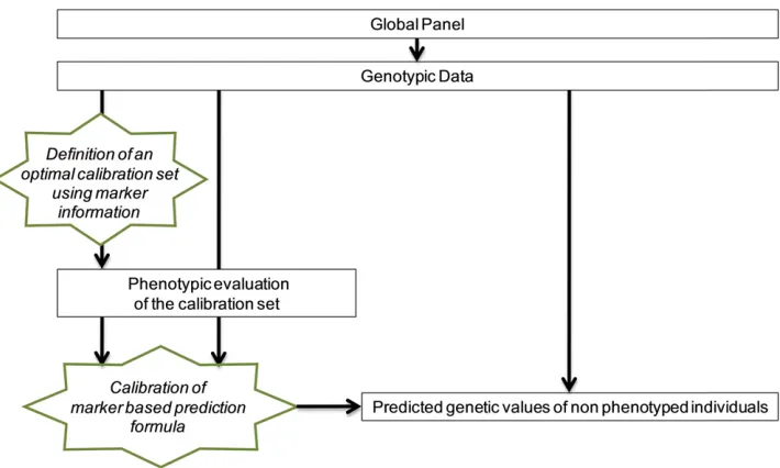
(Figure 1). A ﬁrst way to perform sampling could be to

choose the individuals that capture most of the diversity present in the population. Another criterion could be to se-lect the calibration set that minimizes the prediction error variance (PEV) of the genetic values. This criterion is valid at the individual level but does not take into account the ge-netic variance of the contrasts between individuals and may result in the sampling of close relatives. One classical way of

evaluating the efﬁciency of a given selection method is to

compute its accuracy, deﬁned as the correlation between

predicted and true values, which is an important factor of the expected genetic gain. This criterion is directly available in simulation studies in which true genetic values are known or can be indirectly measured by using cross-validation ap-proaches in experimental data.

A few studies have used the expected accuracy, estimated as

ffiffiffiffiffiffiffiffiffiffiffiffiffiffiffiffiffiffiffiffiffiffiffiffiffiffiffi 12PEV=s2

g

q

(where s2

g is the additive genetic

vari-ance, and PEV represents the part ofs2

gthat is not accounted

for by the predictions) to compare experimental designs and statistical models for dairy cattle (VanRaden 2008; Hayes et al.2009c; Pszczolaet al.2012). In these articles, individ-uals were assumed to be unrelated. As a consequence this

criterion has the same disadvantage as PEV: it doesn’t

con-sider the decrease of genetic variance when close relatives are sampled.

To account for this possible decrease in genetic variance, it is possible to directly maximize the expected reliabilities of the contrasts between each selection candidate and the population mean. It can be implemented with the

general-ized coefﬁcient of determination (Laloë 1993), which

ex-presses the precision of any contrast between individuals. This criterion is the squared correlation between the true and the predicted contrast of genetic values. It is a function of the PEV and of the genetic variance. The generalized

co-efﬁcient of determination (CD) is used by animal geneticists

to optimize experimental designs. In particular it can be

(3)

be compared because they (or their relatives) were not phe-notyped at least once in the same environment. The

gener-alized CD was used, for example, to compare the efﬁciency

of testing designs in beef cattle (Laloë and Phocas 2003) and

sheep (Kuehnet al.2007).

In plant breeding, the generalized CD was used by

Maenhoutet al.(2010) to get the most accurate BLUPs from

phenotypic data available from a breeding company. The phenotypic data of breeding companies are very unbalanced, some phenotypes being disconnected from the others.

Maenhoutet al.(2010) assumed that the genotyping

bud-get was limited, and they wanted to use the phenotypes already available for predicting the value of untested hy-brids. Their challenge was, then, how to choose the indivi-duals to genotype in order to optimize the use of available phenotypes. With this exception, to our knowledge, this cri-terion was paid little attention in plant breeding so far and it could be used for different applications such as the opti-mization of the sampling of the calibration set in genomic selection.

Since phenotyping is now the limiting factor in genome-wide analysis, we consider the case in which all the in-dividuals are genotyped but only a proportion is going to be phenotyped (calibration set). In this article, we propose a method based on the generalized CD to optimize the sampling of the calibration set for predicting as accurately as possible the nonphenotyped individuals (Figure 1). To val-idate our optimization algorithm, we used phenotypic data

for ﬂowering time, plant biomass, and dry matter content,

collected on two maize inbred panels for which genotypic information is available and compared several strategies for selecting the calibration set.

Materials and Methods

Genetic material

Our optimization procedure was evaluated on two maize

diversity panels developed for the European program“

Corn-Fed.”These are composed respectively of 300 Flint lines and

300 Dent lines. This material includes 242 lines from the

panel presented by Camus-Kulandaivelu et al. (2006) and

lines derived from recent breeding schemes: 58 Dent lines

from PVP (Mikel 2006; Nelson et al. 2008), 128 from the

University of Hohenheim (Riedelsheimer et al. 2012), 81

from the Misión Biológica de Galicia and the Estación Ex-perimental de Aula Dei, Spain (CSIC), 35 from the Centro Investigacións Agrarias de Mabegondo, Spain (CIAM), 23 from the Eidgenössische Technische Hochschule Zürich (ETHZ), and 33 from the Institut National de la Recherche Agronomique (INRA). This collection was created with the objective of covering European and American diversity of interest for temperate climatic conditions, as available from public institutes. Choice was guided by pedigree to avoid as far as possible overrepresentation of some parental materials.

Field data

The Flint and Dent lines were respectively crossed to a Dent and a Flint tester. The two panels were evaluated separately

for ﬂowering time and biomass production in two adjacent

trials atﬁve locations in 2010: Mons (France), Pontevedra

and Mabegondo (Spain), and Roggenstein and Einbeck (Germany). The hybrids within each panel were divided into two groups according to their expected precocity. These two groups were evaluated as two blocks. A small number of randomly chosen entries was replicated within blocks (18 entries) and across blocks (18 entries) to estimate

experi-mental error and an eventual block effect. Male ﬂowering

time (Tass_GDD6), plant dry matter yield (DM_Yield), and dry matter content (DMC) were registered for each plot.

DMC and DM_Yield were observed at only four of the ﬁve

locations for the Flint panel. Male ﬂowering time was

registered when 50% of the plants were shedding pollen and then converted into growing degree days (GDD) in base

6, using the mean daily air temperature measured at each

location. These traits were used here as examples, to test the optimized sampling algorithm. Plants with obviously ex-treme phenotypes were excluded from the study (between 2.2 and 2.8% of the data were removed for each trait).

Least-squares means were calculated with the GLM procedure (SAS Institute, 2008) by adjusting for block and

trial effects (the phenotypes are compiled inFile S1andFile

S2). Trait heritability at the level of the experimental design

was estimated with a mixed model (Trial as ﬁxed effect,

genotypes and genotypes · trial as random effects) after

removing the block effects. Heritability was calculated as

h2¼ s

2 g

s2

gþs2g·E=nTrialþs2E=nRep

;

wheres2

gis the additive genetic variance,s2Eis the

environ-mental variance, s2

g·E is the interaction variance, nTrial is

the number of trials, and nRep is the mean number of rep-licates over the whole experimental design.

Genotyping, diversity, and relationship matrix

The two diversity panels were genotyped with the 50k SNPs

array described by Ganalet al.(2011). This Illumina array

includes 49,585 SNPs. Individuals, which had marker

miss-ing rate and average heterozygosity.0.1 and 0.05,

respec-tively, were eliminated. Markers, which had missing rate

and average heterozygosity .0.2 and 0.15, respectively,

were eliminated. In total, 261 Flint lines and 261 Dent lines

passed the genotyping and phenotyping ﬁlter criteria. To

avoid the bias noted by Ganalet al.(2011) in the diversity

analysis, we used only the markers that were developed by comparing the sequences of nested association mapping

founder lines (PANZEA SNPs; Goreet al.2009) to estimate

Nei’s index of diversity (Nei 1978) and relationship coefﬁ

-cients (30,027 and 29,094 markers passed theﬁlter criteria

(4)

File S2). Nei’s index of diversity of each Panzea SNP was calculated and averaged over the genome to estimate diver-sity in the two panels.

One easy way to estimate the relationship between individ-uals with molecular markers is to calculate for each pair of individuals the proportion of shared alleles, also called identity-by-state (IBS). With biallelic markers it can be calculated as

A IBS¼GG9þG2G29

K ;

whereGis the matrix of genotypes (with dimension number

of individuals·number of markers) coded as 0, 0.5, and 1

for the homozygote, the heterozygote, and the other

homo-zygote, respectively, Kis the total number of markers, and

G2¼12G, where1is a matrix of ones.

In this formula, a same weight is given to all markers.

Another formula was proposed by Leuteneggeret al.(2003),

Aminet al.(2007), and Astle and Balding (2009) in which a particular weight, depending on the allele frequency, is given to each marker,

A freqi;j¼ 1 K

XK k¼1

Gi;k2pk

Gj;k2pk

pkð12pkÞ ;

where i and j indicate individuals, Gi,k is the genotype of

individualiat markerk, andpkis the frequency of the allele

coded 1 of marker k in the panel. This estimator attributes

a higher weight to similarity for rare alleles and to markers

with low diversity. The allele frequenciespkare estimated in

a reference population (here each panel). We consider here the diversity panel as the base population; as a result the

mean of the values of genomic relationship matrixA_freqis

equal to zero. This formula can give negative estimates of

relationship coefﬁcient. Negative coefﬁcients have no sense

in terms of probability, but can be interpreted as negative correlations. These two genomic relationship matrices are

positive semideﬁnite (Astle and Balding 2009) and invertible

when the number of markers is sufﬁcient and identical

indi-viduals are removed. Genomic relationship matrices, as de-scribed above, were estimated independently in both panels.

Statistical model

The genomic predictions were based on the RA–BLUP model,

which allows a more direct derivation of PEV and CD for the breeding values (see below), using the following mixed model

y¼XbþZuþe;

where y is a vector of phenotypes, b is a vector of ﬁxed

effects (in our case only the intercept), u is a vector of

random genetic values, and e is the vector of residuals.X

andZare design matrices.

The variance of the random effects u is varðuÞ ¼As2

g,

where A is the genomic relationship matrix and s2

g is the

additive genetic variance in the panel. The variance of the residuals e is varðeÞ ¼Is2

e, where Iis the identity matrix.

The prediction of u is obtained by solving Henderson’s

(1984) equations

X9X X9Z

Z9X Z9ZþlA1

_^ b ^ u ¼

X9y Z9y

;

wherel ¼ s2

e=s2gis the ratio between the residual and the

additive variances in a simpliﬁed situation; in our case

l¼s

2

E=nRepþs2g·E=nTrial

s2

g

:

Ais the genomic relationship matrix. Note that in this model

we consider that a trait is determined by a large number of genes, each having small and independent effects. Genetic effects are assumed to follow a Gaussian distribution accord-ing to the central limit theorem (Fisher 1918).

Optimization criteria and CD

The ﬁnal objective is to identify the individuals from the

population that are best suited to build the calibration panel. One strategy for reaching this objective is to maximize the precision of the prediction of the difference between the value of each nonphenotyped individual and the mean of the total population of candidate individuals, which includes the phenotyped and the nonphenotyped individuals. This

difference can be viewed as a speciﬁc contrast between

genetic values of individuals.

A classical approach for this is to compute the expected PEV of each individual, which can be obtained from

X9X X9Z

Z9X Z9ZþlA1

₁ ¼ C11 C12 C21 C22 ;

wherePEVðu^Þ ¼Varðu^uÞ ¼diagðC22Þ·s2 e.

More generally, thePEVof any contrastcof the predicted

performances can be calculated as

diag "

c9Z9MZþlA11_c c9c

# ·s2

e;

where cis a contrast,i.e.,10c¼0.M is an orthogonal

pro-jector on the subspace spanned by the columns of X:

M¼IXðX9XÞX9andðX9XÞ2 is a generalized inverse of

X9X(Laloë 1993).

A complementary approach to optimizing the choice of individuals to be phenotyped is to estimate the expected reliability of the prediction of contrasts. Laloë (1993) expressed the precision of any contrast with the generalized

CD, deﬁned as the squared correlation between the true and

the predicted contrast of genetic values. This CD is equiva-lent to the expected reliability of the contrast

CDðcÞ ¼diag

"

c9AlZ9MZþlA11_c

c9Ac

#

(5)

The CD takes values between 0 and 1, a CD close to 0 meaning that the prediction of the contrast is not reliable, whereas CD close to 1 means that the prediction is highly reliable. The CD is a balance between PEV and the genetic variance (of the contrast), which takes into account

re-lationship (Laloëet al.1996).

Note that compared to the approach of Hayes et al.

(2009c) who considered ffiffiffiffiffiffiffiffiffiffiffiffiffiffiffiffiffiffiffiffiffi12PEV=s2 g

p

an estimation of

accu-racy, the termc9Acin the CD takes into account covariances

between the candidate individuals. The use of generalized CD instead of PEV as optimization criterion is expected to prevent the selection of very closely related individuals.

The set of individuals to phenotype within each panel (Dent or Flint) was optimized by minimizing the mean of the PEVs of the contrast between each nonphenotyped

individ-ual and the mean of the panel: PEVmean ¼ mean[diag

(PEV(C))], whereCis a matrix of contrasts: each column

is a contrast between an unphenotyped individual and the

mean of the population. Dimensions ofCare total number of

individuals·number of nonphenotyped individuals.

We also optimized the sampling by maximizing the mean of the CDs of the contrast between each nonphenotyped individual

and the mean of the panel: CDmean¼mean[diag(CD(C))].

In this case, the individuals that we decide not to phenotype are those that are the most reliably predicted with those that are phenotyped. In other words, we optimize the choice of individuals to phenotype, so that their phenotypes are as useful as possible to predict the unphenotyped individuals (Figure 1). We expect this strategy to sample key individuals that cover the panel variability as well as possible.

These approaches based on PEVmean or CDmean were used with the two relationship matrices described above: the

IBS matrixA_IBSand the genomic relationship matrixA_freq.

These criteria, PEVmean and CDmean, were compared to other criteria expected to improve the calibration set sam-pling: we also considered as selection criteria the mean and

the maximum of the genomic relationship matrix A_freq

between the individuals in the calibration set (respectively denoted by Amean and Amax). These two criteria Amean and Amax were minimized to maximize the variability in the calibration set.

Optimization algorithm

Several exchange algorithms and simulated annealing

(Kirkpatrick et al. 1983; Černý 1985) classically used to

optimize experimental designs (Atkinson et al.2007) were

implemented in R 2.14.0 to optimize the different criteria. A simple exchange algorithm, further referred to as Algo1, was retained. At each step the random exchange of one individual between the calibration set and the set of nonphenotyped individuals is accepted if the criterion were improved and was rejected otherwise. More complex algorithms did not

give signiﬁcantly better results and needed more iterations

to converge. They were therefore not retained for further investigations.

For each panel, we used Algo1 50 times to select a certain number of individuals (10, 30, 50, 70, 100, 150, or 200) for phenotyping, each time with a different random initial sample. Preliminary tests showed that 50 repetitions were

sufﬁcient to obtain stable results. We then used the true

phenotypes of these individuals (calibration set) to predict the remaining individuals (validation set). We compared results obtained for optimized calibration sets with those obtained for randomly determined calibration sets (50 random sets for each calibration set size). This procedure was applied to each trait in each panel.

Observed prediction reliability and robustness of the optimization to variation of heritability

(6)

values (GEBV) and the true breeding values (TBV): corr2_ð_GEBV_;_TBV_Þ_{, which is the square of the genomic}

selec-tion accuracy (Dekkers 2007). We do not have access to

the TBV of the candidate plants. Considering that

corrðGEBV;YÞ ¼corrðGEBV;TBVÞ ·corrðY;TBVÞ, where Y stands for the observed phenotypic performance, we estimated the genomic selection reliability as corr2_ð_GEBV_;_Y_Þ_=h2_{, since} h2_¼_corr2_ð_Y_;_TBV_Þ_{. For each panel and each calibration set}

size we compared the observed prediction reliabilities using the optimized or the random set.

In the CD calculation, the only parameter that is related to the trait is the variance ratiol. This parameter is related to the heritability of the trait:l¼ ð12h2_Þ_=h2_{. We need to set}

a speciﬁc value for lto use the sampling algorithm. But in

practice, the calibration set will probably be phenotyped for traits of different heritabilities. It is thus important to know, for a set optimized with a speciﬁc value ofl, for which range of heritabilities it is optimum. To answer this question, we compared the CDmean of selection candidates obtained after sampling the calibration set with different values of lambda. If the CDmean obtained with different lambda values are correlated, one can assume that close subsets of individuals would be selected by the sampling approach.

For this, random sets of individuals were successively selected, and each time the CDmean was calculated (with the genomic relationship matrix) using three different

values for l: 4, 1, and 0.25 corresponding to heritabilities

of 0.2, 0.5, and 0.8. The correlations between the three series of CDmean were then calculated.

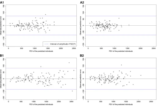
Link between the PEV and the observed prediction error

For the Flint and the Dent panels independently, 50 sets of 150 individuals were sampled randomly or with the optimization algorithm (CDmean). These calibration sets were used to predict the genetic values of the unphenotyped individuals from the same panel. We calculated the PEVs of the contrasts between each predicted individual and the

mean of the population (using a l corresponding to the

estimated heritability) and compared it to the observed

pre-diction error (deﬁned as the difference between the

obser-vation and the prediction). This comparison is interesting to check if our statistical model gives good estimates of the PEV and then indirectly if the estimated variance/covariance

ma-trixﬁts the true variance/covariance matrix.

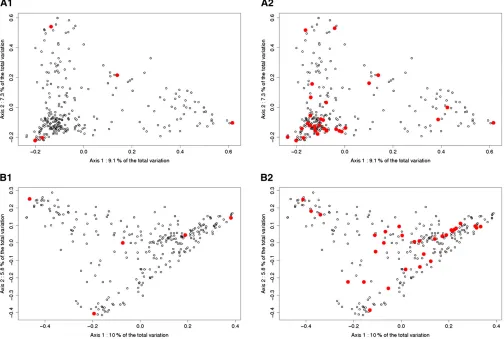
Genetic properties of optimized calibration sets

To visualize the genetic properties of the calibration sets optimized with CDmean, two kinds of tools were used: a principal coordinates analysis (PCoA) on the distance matrices (Gower 1966), and a network representation of the genomic relationship matrix.

A PCoA was performed on the distance matrix of each panel (we considered the distance between two individuals

by one minus their relationship coefﬁcient A_freqij). The

individuals were then plotted using their coordinates on the two axes of the PCoA explaining most of the total

var-iance. This representation gives an idea of the variability present in each panel. Using these graphs, we visualized the individuals selected by the sampling algorithm based on CDmean. It gives a rough idea of the variability of the panel captured by the calibration set.

To further understand how the individuals selected to be part of the calibration set relate to the other individuals of the population we used a visualization of the genomic relation-ship matrix. We represented the individuals in a network, in which two individuals are linked when their relationship coefﬁcient (A_freqij) is.0.2, unlinked otherwise (Rozenfeld

et al. 2008; Thomaset al.2012). For this, the genomic re-lationship matrix was transformed in a matrix of Boolean in-dicating if the coefﬁcients were.0.2 or not. The networks of the two panels were drawn with a Fruchterman and

Rein-gold’s force-directed placement algorithm (Fruchterman and

Reingold 1991) with the package“network”in R.

Results

Trait variation

Tass_GDD6, DMC, and DM_Yield have an important vari-ability in the two panels (Table 1). The average of these traits are only slightly different between the two panels because the Dent lines (usually late lines) were crossed to a Flint tester (early lines) and the Flint lines to a Dent tester.

The genotype · environment interaction and the residual

variances were low compared to the genetic variances for Tass_GDD6. The residual and interaction variances are rel-atively more important for DMC but remain below genetic variance. The residual variance was greater than the genetic variance for DM_Yield and the interaction variance was equal to the genetic variance in the Dent panel. The herita-bility of these traits is between 0.65 (DM_Yield in the Dent panel) and 0.95 (Tass_GDD6 in both panels).

Description of the diversity and of the genomic relationship matrix

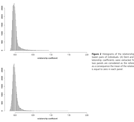
The index of diversity (Nei 1978) in the Dent and the Flint panels was 0.34 and 0.32, respectively, leading to a mean

A_IBSof 0.66 and 0.68, respectively. Histograms of the

ge-nomic relationship coefﬁcients A_freqijin the Flint and the

Dent panels show that most of the coefﬁcients are,0.1, but

some pairs of individuals are closely related in particular in the Flint panel (Figure 2). For these individuals the

identity-by-state can be up to 0.99. The coefﬁcient A_freqijof these

pairs of individuals can almost reach 2 if the two individuals

share many rare alleles. Three Dent andﬁve Flint pairs were

almost identical despite all the care that was used to create these diversity panels.

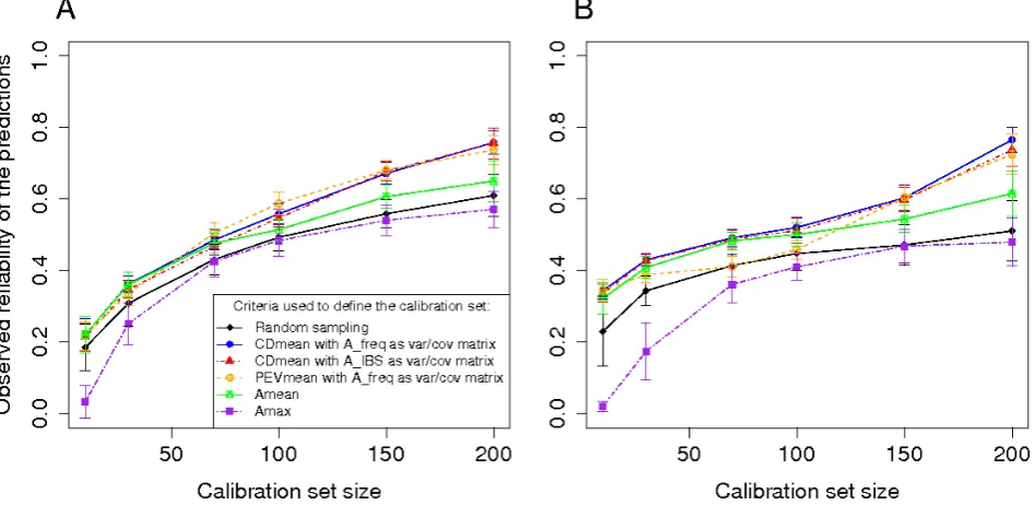
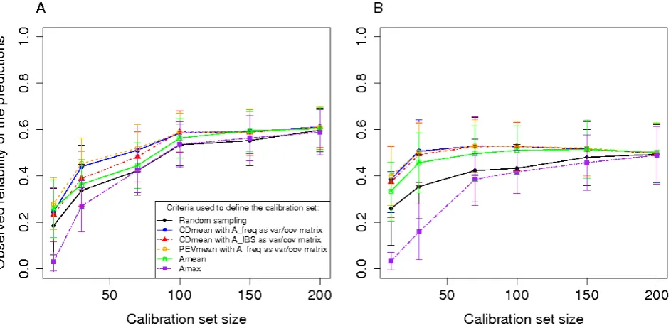
Observed prediction reliability and robustness of the optimization to variation of heritability

(7)

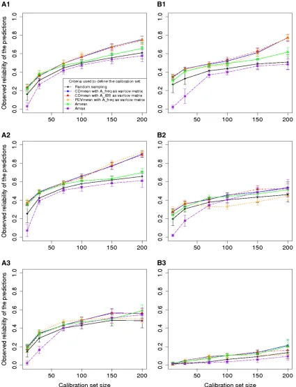
DM_Yield in the Flint panel the reliabilities are ,0.3 even with a calibration set of size 200 (Figure 3). As expected the observed reliability increased with the size of the cali-bration set. For the random samples, an increase of the calibration set size generates an increase of the reliability following the law of diminishing returns (Figure 3). For the set optimized with PEVmean and CDmean, this trend is less clear. Within calibration set sizes, there were clear differ-ences between the reliabilities obtained with the different approaches. All the approaches except the minimization of

Amax gave better reliabilities than the reliabilities obtained after random sampling. The approach based on PEVmean was better than random sampling most of the time, but it was equivalent or worse than random sampling in few situations (particularly for DMC in the Flint panel). The reliabilities obtained by minimizing Amax in the calibra-tion set were always lower or equivalent to those obtained by random sampling, whereas the minimization of Amean always gave higher reliabilities than random sampling (Figure 3).

Table 1 Statistics on Flowering time (Tass_GDD6, growing degree days), dry matter yield (DM_Yield,t·ha-1_{), and dry matter} content (DMC, %) in the two panels of hybrids

Dent Flint

Tass_GDD6 DM_Yield DMC Tass_GDD6 DM_Yield DMC

Mean 864.5 17.0 33.4 872.4 15.9 32.4

Genotypic variance 1354.5*** 1.9*** 13.0*** 1692.1*** 2.1*** 8.6***

Trial·genotype variance 77.5*** 1.9*** 4.1*** 95.8*** 0.7* 6.1***

Residual variance 292.2*** 3.6*** 6.5*** 355.2*** 3.9*** 8.1***

Heritability 0.95 0.65 0.87 0.95 0.67 0.72

The variances were estimated in a mixed model with Genotype, Trial·genotype and Residual as random effects, *P,0.05, ***P,0.001. The observations were previously corrected by block effects. The heritability corresponds to the broad-sense entry-mean heritability.

(8)

The approach based on CDmean always gave higher

reliabilities than random sampling. The use ofA_IBSas

var-iance/covariance matrix gave lower reliabilities. Considering the results obtained in the two panels with the different

cal-ibration set sizes, CDmean withA_freqwas the best method.

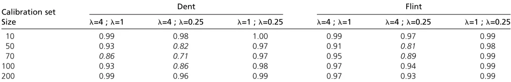
The correlations between the CDmeans computed for the

three levels of heritability were .0.90 most of the time

(Table 2) and always.0.70. The CDmeans calculated with

the intermediate value ofh2₍_h2_{= 0.5) had minimum}

cor-relations of 0.86 and 0.91 with the CDmeans calculated with the two extreme heritabilities (0.2 and 0.8), for the Flint and Dent panels, respectively.

Link between the PEV and the observed prediction error

Another way of checking the reliability of our statistical models was to compare the expected PEVs and the observed prediction errors (Table 3 and Figure 4). Figure 4 illustrates the results obtained after 1 of the 50 repetitions of the al-gorithm on Tass_GDD6. This showed that the larger ob-served prediction errors mostly corresponded to high PEV, particularly for Flints.

The PEVs obtained with the approach based on CDmean were lower than the PEVs obtained with a random calibra-tion set. This expectacalibra-tion was validated by the observed prediction errors, which were lower with CDmean than with random sampling.

Genetic properties of optimized calibration sets

The twoﬁrst PCoA axes represented, respectively, 16.4 and

15.8% of the total variability in the Dent and the Flint panels (Figure 5). When the calibration set was small, the algo-rithm tended to select individuals on the extremities of the graph. When the calibration set was larger, the algorithm selected representative individuals. For example, in A2 many individuals were selected from the lower left cluster, where most individuals were placed. These patterns were stable across runs.

Figure 6 presents pairs of individual with a genomic re-lationship coefﬁcient.0.2 (A_freqij) as linked by an edge.

This visual representation gives a global idea of the relation-ships in the panels: individuals related to others are clus-tered into groups, while more originals lines are isolated on the graph. When few lines were phenotyped, the algorithm selected individuals representing the biggest clusters. But when the calibration set size was bigger, it was composed of few individuals in the clusters and many isolated individ-uals. At a given calibration set size, the algorithm selected all the“isolated”lines and few lines in the kinship clusters. When increasing even further the calibration set size, the few individuals that were not in the calibration set were located at the center of the kinship clusters.

Discussion

The objective of this study was to maximize the reliability of genomic predictions by optimizing the composition of the

calibration set of individuals based on genotypic data only (Figure 1). To do so, we used different criteria that were expected to be related to the reliability of the genomic pre-diction. These criteria can be used before collecting pheno-typic data to optimize the calibration set. The algorithms based on these criteria were tested on two independent panels that included inbred lines of different origins and on three traits with heritabilities ranging from 0.65 to 0.95. There were clear differences of observed reliabilities between the two panels and between the three traits (Figure 3). The limited number of degrees of freedom available for estimating error variance may affect the estimation of her-itabilities, which may affect the scale of observed reliabilities

for a given panel–trait combination (through the division by

h2_{). The low reliabilities obtained for the Flint panel for}

DM_Yield may be explained by a combination of (i) low precision of data used for prediction (similar, however, to that of Dent panel for the same trait), (ii) looser pedigree structure than in the Dent panel, and (iii) larger nonadditive effects possibly related to more important plant lodging, which deserve further investigations.

Whatever the differences in reliability range among panel–trait combinations, all the optimization criteria except

Amax (the maximum of the relationship coefﬁcients

be-tween the reference individuals) increased the observed re-liability compared to random sampling.

The only exception to this was PEVmean for intermediate calibration set sizes for DMC in Flint panel. In particular, the approaches based on CDmean and Amean always gave higher reliabilities than random sampling whatever calibra-tion set sizes. For Amean this is in accordance with Pszczola et al.(2012), who showed that the relatedness between the reference individuals and between the candidates and the reference individuals has a strong effect on the accuracy. For calibration sets of reduced size, Amean and CDmean yielded similar reliabilities because they both sampled the less-re-lated individuals. For larger calibration sets, the approach based on CDmean gave better results, which can be explained by the consideration of the whole network of kin-ship, whereas Amean considers only the mean. CDmean explicitly takes into account the information brought by the experiment.

The optimization based on PEV was one of the most

efﬁcient approaches. However, the approach uniquely based

on PEV (PEVmean) has two important drawbacks, which can explain why it can sometimes be worse than random

sampling (Figure 3): (i) it doesn’t take into account the

de-crease of genetic variance due to kinship, (ii) and it is highly

dependent on the trait heritability. The ﬁrst point can be

neglected if all the individuals are independent. In this case the approaches based on PEVmean and on CDmean are equivalent. But most of the time the individuals considered by breeders are to some extent related, even in diversity panels like those considered in the present study. Not

con-sidering these relationship coefﬁcients can lead to biased

(9)

Figure 3 Reliability of the predictions of Tass_GDD6 (A1 and B1), DMC (A2 and B2) and DM_Yield (A3 and B3) using different sampling algorithms on the Dent panel (A1, A2, and A3), and the Flint panel (B1, B2 and B3). The calibration sets were randomly sampled or deﬁned by maximizing CDmean with a relationship matrix based on the IBS or weighted by the allelic frequencies; minimizing PEVmean with a relationship matrix weighted by the allelic frequencies; minimizing the mean (Amean) or the maximum (Amax) of the relationship coefﬁcient between the reference individuals. The individuals that are not in the calibration set are in the validation set. As a consequence, for each calibration set size the reliability is calculated with a different number of individuals. For each point, the vertical line indicates an interval of 2sR(sRbeing the standard deviation of observed reliabilities over the 50

(10)

formulas used in animal genetics, which consider the indi-viduals as unrelated, overestimate accuracy compared to what is found by using cross-validation (VanRaden 2008;

Hayeset al.2009c; Pszczolaet al.2012). In the CD

calcula-tion, the covariance between the candidate individuals is taken into account byc9Acsg2, and as a result the reliability

is better estimated.

The second point, sensitivity to heritability, is very im-portant because the calibration set is often phenotyped for many traits of interest with different heritability levels. The calibration set has thus to be optimal for a wide range of

heritability levels. Both PEV and CD depend onl, which is

directly related to the trait heritability. To test the effect

of l on the different methods, we used the algorithm on

Tass_GDD6 with a lof 1 corresponding to a heritability of

0.5. The reliabilities obtained with CDmean with the twol

values are very close, whereas PEVmean can be less accurate

than random sampling if thelvalue used for the

optimiza-tion is different from the true l (Supporting Information,

Figure S1). The robustness of CDmean to variation of

heri-tability is conﬁrmed in Table 2, which shows that if an

in-termediate value oflis chosen, the calibration set is close to optimality for a wide range of heritabilities. In fact this

sec-ond point is related to the ﬁrst one: the reduction of

vari-ance due to relationship is not taken into account in the PEV calculation, which makes it highly dependent on the trait heritability. For example, if the set is optimized by minimiz-ing the PEV with a very low heritability, the calibration set is composed only of highly related individuals (results not shown), whereas if the heritability is high, the calibration set would explore the whole variability of the panel. In the CD calculation the termc9Acprevents selection of individuals too closely related.

The absence of a clear plateau for CDmean method according to calibration size in Figure 3 leads us to check

whether improvement in reliability observed with CDmean-based optimization may be partly explained by the selection of validation sets (the complement to calibration set in our main approach) presenting a broad variation. To address this issue, we performed a different cross-validation proce-dure on Tass_GDD6. We considered here validation sets

determined a priori. In aﬁrst step 30 individuals were

ran-domly sampled to deﬁne the validation set. In a second step

calibration sets were sampled from the remaining individu-als at random or using different approaches to optimize the prediction reliability for the validation set. Although a dimishing return according to calibration population size

in-crease was observed, the ranking in methods (Figure S2)

was consistent with what was found before (Figure 3). This shows that an increase in reliability for CDmean cannot be

attributed mostly to the extraction of an “easy to predict”

validation set. We also performed the optimization on the adjusted means of DMC and DM_Yield of each single trial and found consistent results: the different approaches were ranked in the same order except for one trial for which the reliabilities were very low whatever the calibration set size and the method (results not shown).

Previous elements show that CDmean is preferable to PEVmean and is a criterion of choice to predict reliability and to optimize the calibration set. Under our conditions, using the optimized sampling algorithm based on CDmean

and using A_freq as variance/covariance matrix, an

opti-mized set of approximately 100 lines can reach the same reliability as random samples of approximately 200 lines. Cost of heavy phenotypic evaluations could therefore be substantially reduced by using an optimized calibration set. This approach can also be used to estimate the precision of a particular prediction after collecting phenotypic data (Figure 4). This information is important because it would help the breeders to select the best individuals considering Table 2 Correlation between the CDmeans calculated with different values ofl

Calibration set Dent Flint

Size l=4 ;l=1 l=4 ;l=0.25 l=1 ;l=0.25 l=4 ;l=1 l=4 ;l=0.25 l=1 ;l=0.25

10 0.99 0.98 1.00 0.99 0.97 0.99

50 0.93 0.82 0.97 0.91 0.81 0.98

70 0.86 0.71 0.97 0.95 0.89 0.99

100 0.93 0.86 0.98 0.97 0.94 0.99

200 0.99 0.96 0.99 0.97 0.93 0.99

For each calibration set size, the CDmeans of 200 random samples were calculated with three different values ofl. Each value of the table indicates the correlation between CDmeans calculated with two values ofl. The values in italics are the correlations,0.9. The three values ofl(4, 1, 0.25) are, respectively, equivalent to heritabilities of 0.2, 0.5, and 0.8.

Table 3 Means of the expected and observed error variances in the Dent and Flint panels for Tass_GDD6

Dent Flint

Mean PEVmean Observed prediction error variance Mean PEVmean Observed prediction error variance

Random set 865.6 654.7 1204.1 973.8

Optimized set 610.8 367.9 857.9 699.8

(11)

not only the best predicted values but also associated reli-abilities. This information would also be useful to identify situations in which a complementary sampling of the cali-bration data set is needed to increase the reliability of the predictions of original individuals that were poorly pre-dicted with the initial calibration set.

When the calibration set is small, it appears that the algorithm based on CDmean samples individuals that are

“extreme”on the PCoA representation (Figure 5). As a

con-sequence, the variability explained by the main axes is well captured by the calibration set. When the calibration set is larger, the selected individuals are spread across the whole graph, and they are always separated by a minimum dis-tance. When two individuals are highly related, the algo-rithm never selects both of them as clearly illustrated by network visualizations (Figure 6). The number of clusters depends on the threshold used to determine if two

individ-uals appear related or not. We used a threshold on A_freqij

of 0.2 because the clusters of related lines were then clearly visible. When the calibration set is small, the individuals selected are in the biggest clusters. This choice permits reli-able prediction of more individuals than if isolated lines

were selected. If the calibration set becomes larger, both isolated and linked individuals are selected. It can be explained by the fact that when the clusters are represented

by a sufﬁcient number of phenotyped individuals, it brings

more information to phenotype an isolated individual than an additional one in the clusters. At a certain calibration set size, the only lines that are not in the calibration set are in the center of the clusters. These lines are among the most typical of each group; they are also the most easily predicted when many genetically close lines are phenotyped.

In addition to these general trends, we showed that the selection of the reference individuals by the approaches based on CDmean or PEVmean depends on the method used to estimate the variance/covariance matrix. This

relation-ship matrix should reﬂect the variance/covariance between

individuals at the QTL positions. It is thus possible that the

best formula with which to estimate A is not the same for

different traits, according to the weight that is given to the

markers. The use of A_freq instead of A_IBS slightly

in-creased the observed reliability of the predictions. It shows

thatA_freqgave better estimates of the relationship coefﬁ

-cient between individuals thanA_IBS, at least with our data.

(12)

In the case of highly polygenic traits, we consider that the QTL are spread on the whole genome, and so we use markers covering the whole genome to estimate the vari-ance/covariance matrix. We need a number of markers high enough to have at least one marker in high linkage

disequi-librium (LD) with each QTL. Goddardet al.(2011) showed

that an incomplete coverage of the genome by markers can be a cause of overestimation of the accuracy. CDmean and PEVmean could be subject to this bias because we used a variance/covariance matrix estimated with markers to

cal-culate these criteria. Goddardet al.(2011) proposed

calcu-lating a variance/covariance matrix based on the genomic relationship matrix and on the pedigree to predict accuracy without bias. In our case the pedigree was not available and so we could not use their correction. However, our marker density compared to LD was such that a risk of having an important bias was limited.

The approaches we proposed were tested on two in-dependent diversity panels and three traits and globally consistent results were obtained. It would be interesting to test these approaches on other types of populations, in particular in the presence of strong population structure. We

have considered here two heterotic groups separately. It may be interesting to test the approach to optimizing samples including lines of different heterotic groups, with the objective of obtaining accurate predictions across and within heterotic groups. It would then be required to have an important coverage of the genome to capture ancestral LD, otherwise the reliability would be overestimated as dis-cussed before. Breeders are also interested in applying genomic selection in multifamilial populations (Albrecht et al.2011; Zhaoet al.2012). Albrechtet al.(2011) showed that in such situations the prediction reliabilities are highly dependent on the composition of the calibration set. In par-ticular, if few families are not represented in the calibration set, the observed reliabilities are lower than if few indi-viduals are sampled in each family. Optimizing the

calibra-tion set therefore deserves speciﬁc attention in this case.

(13)

reliability would evolve across the next generations derived from these materials. This aspect also has to be studied, because the gain of time due to selection on predicted values instead of phenotypic observations is the main interest of genomic selection. It would therefore be important to eval-uate how often the prediction formula must be recalibrated. Finally, although displaying contrasted heritabilities and possibly different contribution of nonadditive effects (see above), the three traits considered here are known to be

highly polygenic (see Chardonet al.2004 and Buckleret al.

2009 for Tass_GDD6), which justiﬁed the choice of the RA–

BLUP model. For traits depending on major genes, this model might be inappropriate or nonoptimal and it may be preferable to use Bayesian or neural network models

(Jannink et al. 2010). Our optimization criterion is based

on the BLUP theory and so would be inappropriate if major genes are involved. It is, however, possible that CDmean

would also be to some extent useful in increasing the re-liability of Bayesian methods. It would be interesting to de-rive a similar criterion from the Bayesian theory to predict reliability before collecting phenotypes.

Acknowledgments

We are very grateful to those who made possible the gathering of inbred lines to our panels, in particular the following: Candice Gardner from United States Department of Agriculture North Central Regional Plant Introduction Station of Ames, Geert Kleijer from Agroscope Changins-Wädenswil of Nyon, Switzerland, Wolfgang Schipprack from Universität Hohenheim of Eckartsweier, Germany, Amando Ordás from Misión Biológica de Galicia of Ponteve-dra, Spain, Ángel Álvarez from Estacion Experimental de Aula Dei of Zaragoza, Spain, José Ignacio Ruiz de Galarreta from Centro Neiker de Arkaute of Vitoria, Spain, Laura Campo from Centro de Investigación Agraria Mabegondo of La Coruna, Spain, and Jacques Laborde and colleagues from Institut National de la Rercherche Agronomique of Saint Martin de Hinx, France. The authors thank the reviewers and the editor for their comments, which im-proved the manuscript. This research was jointly supported

as“Cornfed project”by the French National Agency for

Re-search (ANR), the German Federal Ministry of Education and Research (BMBF), and the Spanish Ministry of Science and Innovation (MICINN). R. Rincent is jointly funded by Limagrain, Biogemma, Kleinwanzlebener Saatzucht AG (KWS), and the Association Nationale de la Recherche et de la Technologie (ANRT).

Literature Cited

Albrecht, T., V. Wimmer, H.-J. Auinger, M. Erbe, C. Knaak et al.,

2011 Genome-based prediction of testcross values in maize.

Theor. Appl. Genet. 123: 339–350.

Amin, N., C. M. van Duijn, and Y. S. Aulchenko, 2007 A genomic background based method for association analysis in related individuals. PLoS ONE 2: e1274.

Astle, W., and D. J. Balding, 2009 Population structure and

cryp-tic relatedness in genecryp-tic association studies. Stat. Sci. 24: 451_–

471.

Atkinson, A. C., A. N. Donev, and R. D. Tobias, 2007 Optimum

Experimental Designs,With SAS. Clarendon Press, Oxford.

Bernardo, R., and J. Yu, 2007 Prospects for genomewide selection

for quantitative traits in maize. Crop Sci. 47: 1082.

Boichard, D., and M. Brochard, 2012 New phenotypes for new

breeding goals in dairy cattle. Animal 6(544): 550.

Buckler, E. S., J. B. Holland, P. J. Bradbury, C. B. Acharya, P. J.

Brownet al., 2009 The genetic architecture of maizeﬂowering

time. Science 325: 714–718.

Camus-Kulandaivelu, L., and J.-B. Veyrieras, D. madur, V. Combes,

M. Fourmannet al., 2006 Maize adaptation to temperate

cli-mate: relationship between population structure and

polymor-phism in the Dwarf8 gene. Genetics 172: 2449–2463.

Černý, V., 1985 Thermodynamical approach to the traveling

sales-man problem: an ef_ﬁcient simulation algorithm. J. Optim.

The-ory Appl. 45: 41_–51.

(14)

Chardon, F., B. Virlon, L. Moreau, M. Falque, J. Joets et al.,

2004 Genetic architecture of ﬂowering time in maize as

in-ferred from quantitative trait loci meta-analysis and synteny

conservation with the rice genome RID G-3710–2010. Genetics

168: 2169–2185.

Crossa, J., G. de los Campos, P. Perez, D. Gianola, J. Burgueno

et al., 2010 Prediction of genetic values of quantitative traits in plant breeding using pedigree and molecular markers.

Genet-ics 186: 713–724.

Dekkers, J. C. M., 2007 Prediction of response to marker-assisted

and genomic selection using selection index theory. J. Anim.

Breed. Genet. 124: 331_–341.

Elshire, R. J., J. C. Glaubitz, Q. Sun, J. A. Poland, K. Kawamoto

et al., 2011 A robust, simple genotyping-by-sequencing (gbs) approach for high diversity species. PLoS ONE 6: e19379.

Fisher, R. A., 1918 The correlation between relatives on the

sup-position of Mendelian inheritance. T. Roy. Soc. Edin. 52: 399–

433.

Fruchterman, T. M. J., and E. M. Reingold, 1991 Graph drawing

by force-directed placement. Softw. Pract. Exper. 21: 1129–

1164.

Ganal, M. W., G. Durstewitz, A. Polley, A. Bérard, E. S. Buckler

et al., 2011 A large maize (Zea mays L.) SNP genotyping ar-ray: development and germplasm genotyping, and genetic map-ping to compare with the B73 reference genome. PLoS ONE 6: e28334.

Goddard, M., 2009 Genomic selection: prediction of accuracy and

maximisation of long term response. Genetica 136: 245–257.

Goddard, M., B. Hayes, and T. Meuwissen, 2011 Using the

geno-mic relationship matrix to predict the accuracy of genogeno-mic

se-lection. J. Anim. Breed. Genet. 128: 409_–421.

Gore, M. A., J.-M. Chia, R. J. Elshire, Q. Sun, E. S. Ersoz et al.,

2009 A ﬁrst-generation haplotype map of maize. Science

326: 1115–1117.

Gower, J. C., 1966 Some distance properties of latent root and

vector methods used in multivariate analysis. Biometrika 53:

325–338.

Habier, D., R. L. Fernando, and J. C. M. Dekkers, 2007 The impact

of genetic relationship information on genome-assisted breeding

values. Genetics 177: 2389–2397.

Hayes, B., P. Bowman, A. Chamberlain, and M. Goddard,

2009a Invited review: genomic selection in dairy cattle:

prog-ress and challenges. J. Dairy Sci. 92: 433–443.

Hayes, B. J., P. M. Visscher, and M. E. Goddard, 2009b Increased

accuracy of artiﬁcial selection by using the realized relationship

matrix. Genet. Res. 91: 47.

Hayes, B. J., P. J. Bowman, A. C. Chamberlain, K. Verbyla, and M.

E. Goddard, 2009c Accuracy of genomic breeding values in

multi-breed dairy cattle populations. Genet. Sel. Evol. 41: 51.

Henderson, C. R., 1984 Applications of Linear Models in Animal

Breeding. University of Guelph Press, Guelph, Ontario, Canada.

Huang, X., Q. Feng, Q. Qian, Q. Zhao, L. Wanget al., 2009

High-throughput genotyping by whole-genome resequencing.

Ge-nome Res. 19: 1068–1076.

Jannink, J. L., A. J. Lorenz, and H. Iwata, 2010 Genomic selection

in plant breeding: from theory to practice. Brief. Funct.

Ge-nomics 9: 166–177.

Kirkpatrick, S., C. D. Gelatt, and M. P. Vecchi, 1983 Optimization

by simulated annealing. Science 220: 671.

Kuehn, L. A., D. R. Notter, G. J. Nieuwhof, and R. M. Lewis,

2007 Changes in connectedness over time in alternative sheep

sire referencing schemes. J. Anim. Sci. 86: 536–544.

Laloë, D., 1993 Precision and information in linear models of

genetic evaluation. Genet. Sel. Evol. 25: 557–576.

Laloë, D., and F. Phocas, 2003 A proposal of criteria of robustness

analysis in genetic evaluation. Livest. Prod. Sci. 80: 241–256.

Laloë, D., F. Phocas, and F. Ménissier, 1996 Considerations on

measures of precision and connectedness in mixed linear

mod-els of genetic evaluation. Genet. Sel. Evol. 28: 1–20.

Leutenegger, A. L., B. Prum, E. Génin, C. Verny, A. Lemainqueet al.,

2003 Estimation of the inbreeding coefﬁcient through use of

genomic data. Am. J. Hum. Genet. 73: 516–523.

Maenhout, S., B. De Baets, and G. Haesaert, 2010 Graph-based

data selection for the construction of genomic prediction

mod-els. Genetics 185: 1463–1475.

Metzker, M. L., 2009 Sequencing technologies: the next

genera-tion. Nat. Rev. Genet. 11: 31–46.

Meuwissen, T., B. Hayes, and M. Goddard, 2001 Prediction of

total genetic value using genome-wide dense marker maps. Ge-netics 157: 1819.

Mikel, M. A., 2006 Availability and analysis of proprietary dent

corn inbred lines with expired US plant variety protection. Crop Sci. 46: 2555.

Nei, M., 1978 Estimation of average heterozygosity and genetic

distance from a small number of individuals. Genetics 89: 583. Nelson, P. T., N. D. Coles, J. B. Holland, D. M. Bubeck, S. Smith

et al., 2008 Molecular characterization of maize inbreds with expired U.S. plant variety protection. Crop Sci. 48: 1673.

Pszczola, M., T. Strabel, H. Mulder, and M. Calus, 2012 Reliability

of direct genomic values for animals with different relationships

within and to the reference population. J. Dairy Sci. 95: 389–400.

R development Core Team, 2006 R: A Language and Environment

for Statistical Computing. R Foundation for Statistical Comput-ing, Vienna.

Riedelsheimer, C., A. Czedik-Eysenberg, C. Grieder, J. Lisec, F.

Technow et al., 2012 Genomic and metabolic prediction of

complex heterotic traits in hybrid maize. Nat. Genet. 44: 217–

220.

Rozenfeld, A. F., S. Arnaud-Haond, E. Hernández-García, V. M.

Eguíluz, E. A. Serrão et al., 2008 Network analysis identiﬁes

weak and strong links in a metapopulation system. Proc. Natl. Acad. Sci. USA 105: 18824.

SAS Institute, 2008 SAS/STATÒ 9.2 User’s Guide. SAS, Cary, NC.

Thomas, M., E. Demeulenaere, J. Dawson, A.R. Khan, N. Galic

et al., 2012 On-farm dynamic management of genetic diver-sity: the impact of seed diffusions and seed saving practices on a population variety of bread wheat. Evol. Appl. (in press).

VanRaden, P., 2008 Efﬁcient methods to compute genomic

pre-dictions. J. Dairy Sci. 91: 4414–4423.

Whittaker, J. C., R. Thompson, and M. C. Denham, 2000

Marker-assisted selection using ridge regression. Genet. Res. 75: 249–

252.

Yang, J., B. Benyamin, B. P. McEvoy, S. Gordon, A. K. Henderset al.,

2010 Common SNPs explain a large proportion of the

herita-bility for human height. Nat. Genet. 42: 565_–569.

Zhao, Y., M. Gowda, W. Liu, T. Würschum, H. P. Maurer et al.,

2012 Accuracy of genomic selection in European maize elite

breeding populations. Theor. Appl. Genet. 124: 769_–776.

Zhong, S., J. C. M. Dekkers, R. L. Fernando, and J.-L. Jannink,

2009 Factors affecting accuracy from genomic selection in

populations derived from multiple inbred lines: a barley case

study. Genetics 182: 355_–364.

(15)

GENETICS

Supporting Information http://www.genetics.org/lookup/suppl/doi:10.1534/genetics.112.141473/-/DC1