High-Level Program Optimizations for Data Analytics.

(1)

ABSTRACT

DING, YUFEI. High-Level Program Optimizations for Data Analytics. (Under the direction of Xipeng Shen.)

Data analytics in many modern applications often spend a large number of cycles on un-necessary computations, while such redundant computations have been hidden in the useful instructions of the applications and are elusive for those automatic code optimizations devel-oped over the past decades. Many algorithms have been manually designed for each specific application, however, none of them are automatic/semi-automatic or generally applicable. My research resides at the intersection of Compiler Technology and (Big) Data Analytics, pioneer-ing the e↵orts of raising the level of automatic program optimizations from implementations to algorithms, and from instructions to formulas. In particular, we find that the algorithm generated by such automatic High-Level Program Optimization matches or outperforms the algorithms manually designed by the domain experts, and thus could have saved decades of manual e↵ort by domain experts.

(2)

(3)

High-Level Program Optimizations for Data Analytics

by Yufei Ding

A dissertation submitted to the Graduate Faculty of North Carolina State University

in partial fulfillment of the requirements for the Degree of

Doctor of Philosophy

Computer Science

Raleigh, North Carolina 2017

APPROVED BY:

Frank Mueller Vincent Freeh

Min Chi Xipeng Shen

(4)

BIOGRAPHY

(5)

ACKNOWLEDGEMENTS

Foremost, I would like to thank my advisor, Dr. Xipeng Shen, for his help, encouragement, and patience throughout my doctoral study. His technical advice, as well as his enthusiasm for research, were essential to the completion of this dissertation. I could not have imagined having a better advisor and mentor for my Ph.D. life.

I would like to thank the rest of my thesis committees—Dr. Vincent Freeh, Dr. Frank Mueller, and Dr. Min Chi—and the graduate school representative—professor Abdennaceur Karoui—for their time and e↵orts to schedule my final defense exam. Their insightful comments and helpful suggestions are essential for completing this dissertation.

My sincere thanks also go to Dr. Saman Amarasinghe, Dr. Una-May OReilly and their group members Jason Ansel, Kalyan Veeramachaneni for their guidance and help during my study at Massachusetts Institute of Technology.

I would also like to thank Dr. Madanlal Musuvathi and Dr. Todd Mytkowicz for o↵ering me the great internship opportunity in their group at Microsoft Research and leading me working on the diverse exciting projects.

I especially thank Dr. Madanlal Musuvathi, Dr. Saman Amarasinghe, Dr. Frank Mueller and Dr. Xipeng Shen for preparing reference letters for my academic job search.

My sincere gratefulness goes to Dr. George N. Rouskas, Ms. Leslie Rand-Pickett, Ms. Kathy Luca for helping with transferring credits, reviewing my job application material and processing my graduation application.

I also thank all my friends at NC state and College of William and Mary. I have enjoyed every moment that we have worked and played together.

(6)

TABLE OF CONTENTS

LIST OF TABLES . . . vii

LIST OF FIGURES . . . .viii

Chapter 1 Introduction . . . 1

1.1 Motivation . . . 1

1.2 Overview of the Dissertation . . . 2

Chapter 2 Yinyang K-Means. . . 7

2.1 Problem Statement . . . 8

2.2 Overview of Proposed Solution . . . 9

2.3 Yinyang K-means . . . 9

2.3.1 Optimizing theAssignment Step . . . 9

2.3.2 Optimizing theCenter Update Step . . . 13

2.4 Algorithm . . . 14

2.5 Evaluation . . . 15

2.5.1 Speedup on theAssignment Step . . . 15

2.5.2 Speedup on theCenter Update Step . . . 19

2.5.3 Overall Speedup . . . 19

2.5.4 Sensitivity Study ont . . . 19

2.6 Related Work . . . 21

Chapter 3 Triangular OPtimizer (TOP) . . . 23

3.3 Unifying Abstraction . . . 27

3.4 Principles of Distance Optimizations . . . 29

3.4.1 Triangular Inequality (TI): Concepts and Implications . . . 30

3.4.2 Principles for Optimization Designs . . . 31

3.5 TOP Framework . . . 40

3.5.1 APIs . . . 40

3.5.2 Runtime Library and Compiler . . . 42

3.6.1 Results Overview . . . 43

3.6.2 Analysis in Detail . . . 44

3.6.3 Discussions . . . 45

Chapter 4 Generalized Strength Reduction . . . 53

4.3 TI and Compiler Technique Development . . . 57

(7)

4.4.1 ATI Theorem . . . 58

4.4.2 Applications for Strength Reduction . . . 60

4.5 Guided Adaptation for Deployment . . . 65

4.5.1 Terminology . . . 65

4.5.2 Existing Insights . . . 67

4.5.3 Special Properties Related with ATI . . . 68

4.5.4 Insights for Deploying ATI . . . 71

4.5.5 Guided TI Adaptation . . . 71

4.6 Integration with Compilers . . . 75

4.6.1 Through Pattern Matching . . . 75

4.6.2 Through Assistance of API . . . 76

4.7.1 Benchmarks . . . 78

4.7.2 Overall Performance . . . 80

4.7.3 Guided TI Adaptation . . . 81

4.7.4 Tighter Bounds by ATI . . . 81

Chapter 5 Autotuning Algorithmic Choice for Input Sensitivity . . . 86

5.3 Language and Usage . . . 91

5.3.1 Algorithmic Choice . . . 91

5.3.2 Input Features . . . 91

5.3.3 Variable Accuracy . . . 94

5.3.4 Usage . . . 94

5.4 Input Aware Learning . . . 95

5.4.1 Level 1 . . . 95

5.4.2 Level 2 . . . 97

5.4.3 Discussion of the Two Level Learning . . . 102

5.5.1 Benchmarks . . . 104

5.5.2 Experimental Results . . . 106

5.5.3 Discussion . . . 111

Chapter 6 Generalized Loop Redundancy Elimination (GLORE) . . . .113

6.3 Four Categories of Loop Redundancy . . . 116

6.4 LER-Notation . . . 118

6.5 GLORE Analysis and Optimizations . . . 121

6.5.1 Overview . . . 121

6.5.2 Removal of Loop-Invariant Loops (Category 3) . . . 123

(8)

6.6 Code-LER Conversion . . . 135

6.7.1 Benchmarks . . . 136

6.7.2 Overall Performance . . . 137

6.7.3 Space Cost . . . 140

6.8 Discussions . . . 141

Chapter 7 Conclusions and Future Work . . . .144

7.1 Conclusions . . . 144

7.2 Future Work . . . 146

(9)

LIST OF TABLES

Table 2.1 Time and speedup on an Ivybridge machine (16GB memory, 8-core i7-3770K processor) . . . 16 Table 2.2 Overall speedup over standard K-means on a Core2 machine (4GB mem,

4-core Core2 CPU) . . . 17 Table 2.3 Unnecessary distance calculations detected by the non-local filters of Yinyang

K-means, Elkan’s algorithm, and Drake’s algorithm. (k= 64) . . . 18 Table 2.4 Yinyang K-means accelerates the center update step by many times . . . . 19 Table 2.5 Cost Comparison (n: # points;k: # clusters;t: # lower bounds per point;

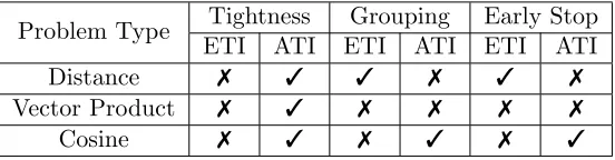
↵: fraction of points passing through the non-local filter; Drake’s algorithm has no local filter) . . . 22 Table 3.1 Six Important Distance-Related Problems. . . 28 Table 3.2 Datasets and Problem Settings. . . 43 Table 4.1 Comparison between ATI and ETI in terms of bound tightness and support

of group filtering and early stop over di↵erent problem types. . . 71 Table 5.1 Mean speedup (slowdown if less than 1) over the performance by the static

(10)

LIST OF FIGURES

Figure 2.1 Two filters for optimizing the assignment step in Yinyang K-means. A rectangle associates with each point to be clustered, representing the set of centers that are possible to replace the current cluster center of the point as its new cluster center. The centers are put into groups and go through the group filter. The local filter examines each center in the remaining groups to further avoid unnecessary distance calculations. . . 12 Figure 2.2 Averaged CPU times of assignment step for Yinyang K-means as a

func-tion of t. . . 20 Figure 2.3 The Voronoi diagrams in two consecutive iterations of k-means, and the

approximation of the overlapped areas by our algorithm (t = 1) and Elkan’s algorithm. . . 21 Figure 3.1 Example distance problems. . . 24 Figure 3.2 K-Means written in TOP API (detailed in Chapter 3.5). Prefix “TOP ”

indicates calls to TOP API. They will be replaced with low-level func-tion calls by TOP compiler, making the algorithm automatically avoid unnecessary distance calculations. . . 25 Figure 3.3 Illustration of distance bounds obtained from Triangular Inequality (bis

a landmark). . . 30 Figure 3.4 Example of the use of landmark hierarchy in a step of K-Means. . . 34 Figure 3.5 Taxonomy of landmark definitions in each category of distance-related

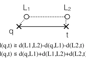
problems. . . 35 Figure 3.6 Illustration of how two landmarks can be used for computing lower and

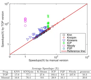
upper bounds of distances. . . 37 Figure 3.7 Algorithm pickLandmarkDef for selecting landmark definitions. . . 49 Figure 3.8 Core APIs defined in TOP. . . 50 Figure 3.9 Speedups brought by TOP and manual optimizations over basic algorithm

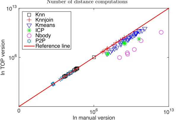
implementations. The graph shows the results for each input and setting; the table reports the geometric average. . . 50 Figure 3.10 The graph shows the number of computations in the optimized

algo-rithms; the table reports the percentage of computations saved by the optimization. . . 51 Figure 3.11 Both spatial and temporal optimizations save many distance

computa-tions for ICP. . . 51 Figure 3.12 Running time changes when di↵erent numbers of 2-level landmarks are

used. . . 52 Figure 4.1 Illustration of traditional triangular inequality, where d(p1,p2) is the length

between points p1 andp2. . . 54 Figure 4.2 (a) original code (b) code that avoids some unnecessary distance

(11)

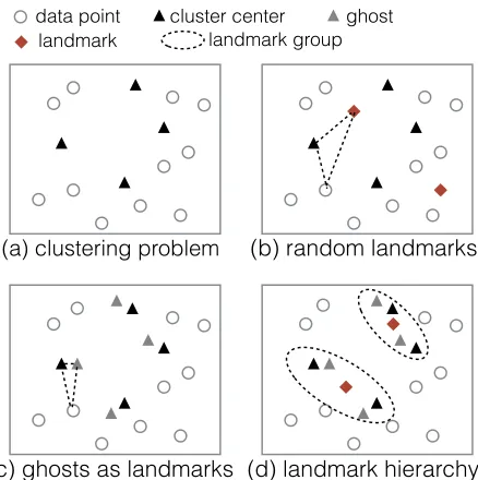
Figure 4.4 (a) A Binary RBM with n visible units and m hidden units (b) ATI on vector dot product. . . 63 Figure 4.5 Illustrations of landmarks, ghosts, and landmark hierarchy on a clustering

example. . . 65 Figure 4.6 Pseudo-code for combined optimization of distance calculations by ETI

and ATI-based strength reduction. . . 72 Figure 4.7 Allowed usage patterns of distances or dot products. . . 76 Figure 4.8 Core APIs for assisting TI-based Strength Reduction. . . 77 Figure 4.9 The graph shows the speedup over the standard version; the table

re-ports the average speedup of our automatic framework compared to the previously optimizedversions [Din15a]. . . 82 Figure 4.10 Speedup brought by the guided TI adaptation over using rigid rules [Din15a]

for deploying TI-based optimizations. The top black segment on each bar represents the overhead incurred by the runtime sampling and adaptation. 83 Figure 4.11 Fraction of extra savings of the distance computations due to the tighter

bounds by ATI over those by ETI on KNNJoin. . . 83 Figure 5.1 PetaBricks pseudocode for Sort with input features . . . 92 Figure 5.2 A selector that realizes a polyalgorithm for sorting. . . 93 Figure 5.3 Usage of the system both at training time and deployment time. At

de-ployment time the input classifier selects the input optimized program to handle each input. Input Aware Learning is described in Chapter 5.4. . . 94 Figure 5.4 Selecting representative inputs to train input optimized programs. . . 96 Figure 5.5 Constructing and selecting the input classifier. . . 97 Figure 5.6 Distribution of speedups over static oracle for each individual input. For

each problem, some individual inputs get much larger speedups than the mean. . . 109 Figure 5.7 Measured speedup over static oracle as the number of landmark

config-urations changes, using 1000 random subsets of the 100 landmarks used in other results. Error bars show median, first quartiles, third quartiles, min, and max. . . 110 Figure 6.1 Illustration of large-scoped loop redundancies. . . 115 Figure 6.2 Examples of the four main categories of loop redundancies. . . 117 Figure 6.3 GLORE transforms formulae through a series of steps to remove its loop

redundancies. A final cross-formula optimization step is omitted. . . 121 Figure 6.4 The alternating form of formula 5x (3d[i] +a[i] d[i]_·(b[j] +c[k]) is

5x+ ( 3d[i]) + ( a[i]) +d[i]_·(b[j] +c[k]), regarded as a hierarchy with the levels alternating between PLUS and TIMES. . . 122 Figure 6.5 The ordering forest produced by the minimum union algorithm for

For-mula 6.9 (the brackets show the relLoopsof each reduction). . . 127 Figure 6.6 Minimum Union Algorithm for selecting an optimized order for reduction

(12)

Figure 6.7 (a) The operand closure tree for Formula 6.10. (b) Closure-based algo-rithm for finding a good order for the operands that share a parent in an operand closure tree. . . 132 Figure 6.8 Examples for removing redundancies of categories 4 and 2. . . 135 Figure 6.9 Speedups on benchmarks optimized by GLORE, compared to the

perfor-mance by two previous techniques ASE and ESR, and their combination (“combined-prior”) on two machines. The baseline is the performance of the original benchmarks. . . 138 Figure 6.10 Speedups by GLORE on six benchmarks with (partially) loop-invariant

(13)

CHAPTER

1 INTRODUCTION

1.1 Motivation

Over the past decades, many traditional program optimization techniques have been developed for improving the efficiency of program executions. However, they have been mostly limited to finding and removing instruction-level inefficiency in program implementations, while we observe that many modern applications—especially those data analytics that process a large volume of data—spend a large number of cycles on unnecessary computations. To find a doc-ument most similar to a query docdoc-ument, for instance, these applications typically would need to examine hundreds of thousands of other documents (that are not the most similar ones) in the dataset. Such redundant computations have been hidden in the useful instructions of the applications and are elusive for traditional code optimizations.

(14)

implementations to algorithms (chapter 2, 3, 4, and 5), and from instructions to formulas (chapter 6).

There are three fundamental challenges for enabling High-Level Program Optimizations faces. First, we need to obtain the high-level semantics of the application, which is often hidden in the low-level implementation. Further, knowledge of beneficial and legal high-level transfor-mations that could change large blocks of code are also required. Third, efficient ways to explore the enormous space of algorithmic or other high-level transformation choices are also essential for the automatic optimization. In this thesis, I will show how my research overcomes these challenges and enables High-Level Program Optimizations, which frequently lower the prac-tical computational complexities of applications, boosting their performance by up to several orders of magnitude.

1.2 Overview of the Dissertation

Automating Algorithmic Optimizations for Distance-Based Algorithms:

Distance calculations are essential to many important algorithms across various domains: data analytics, graph analysis, digital imaging, and scientific simulations. For example, the commonly used clustering algorithm K-means is an iterative algorithm which computes the distances between every data point and each of a set ofK cluster centers in order to decide which center is closest to each point. Nbody simulation computes the distances between every particle and all its neighbors in every time step, in order to simulate the interplay of particles and their resulting movements. Other examples include K-Nearest Neighbor (KNN), point-to-point shortest path in graphs, 3D image construction, and so on.

(15)

more than 20 papers on developing algorithms to optimize distance calculations for K-means. If there were an automatic framework to enable such algorithmic optimization, then decades of manual e↵orts could have been saved.

To build such framework, we start our exploration with a case study on K-means (chapter 2). We learn that the key of applying such algorithmic optimizations to K-means is about how to use TI to e↵ectively compute high-quality(tight) bound of distance and rely on the interplay of lower and upper bounds to filter out unnecessary distance computations. These insights turn into Yinyang K-means, which we believe could be a drop-in replacement of class K-means for its consistent speedup and the preservation of the semantic of the original K-means. Our experiments show that Yinyang K-means is consistently faster (an order of magnitude higher performance) than prior algorithms, regardless of the dimension and size of the data sets, the number of clusters, and the machine configurations. These appealing properties, plus its simplicity, make it a practical replacement of the standard K-means as long as triangle inequality holds.

We further observe that, despite the many di↵erences among those distance-related prob-lems, the underlying mechanisms in which distance calculations have been optimized with TI share commonality across seemingly disparate problem domains. This observation prompts us to propose a simple abstraction, called abstract distance-related problem, to formalize various distance-related algorithms across seemingly disparate domains in a unified manner. We further develop seven principles of using triangular inequality, which lead to a spectrum of algorithmic optimizations along with some automatic mechanisms for selecting the best optimization to use. We turn all these findings into a runtime library, the invocations of which in a program would automatically save unnecessary distance calculations for an arbitrary distance-related problem (that meets the triangular inequality condition).

The result of our exploration is theTriangular OPtimizer(TOP), as described in chapter 3), a compiler and runtime software framework that enables automatic algorithmic optimizations for various distance-based problems. Our experiments show that TOP is able to produce algo-rithms that match or beat (by 2.5X on average) the state-of-the-art algoalgo-rithms that have been designed by domain experts. It also can generate new algorithms for problems, on which no prior work has applied triangular inequality optimizations, and achieve 237X speedups.

(16)

it makes some major contributions in the underlying theory of the optimization, as well as its deployment and integration in compilers. In particular, it proposes a new type of TI, named Angle Triangular Inequality, which could not only help find even tighter distance bounds than TI does, but also make the optimization applicable to more vector-based computations beyond distance calculations, like cosine similarity and dot product calculation. With this generaliza-tion, more data analytic algorithms—for example, restricted boltzmann machine (RBM) in deep learning, document clustering and top-k document retrieval in text mining—could benefit from our automatic algorithmic optimization.

Autotuning Algorithmic Choice Through a Scalable Approach:

Another important technique to explore algorithmic optimization is through algorithmic au-totuning, the goal of which is to determine the best ways to synthesize multiple algorithms together or to configure an algorithm so that the resulting (poly)algorithm can solve a problem e↵ectively. An example of algorithm synthesis is to combine quicksort, mergesort, and inser-tion sort together so that they work at di↵erent stages in sorting a data list. Autotuning helps determine when and how to combine these algorithms. Algorithmic autotuning often features a multifold objective metric: accuracy and performance, because the autotuner must find an algorithm and configuration that meets a given accuracy requirement.

Previous work has demonstrated how a specialized compiler can automate algorithm synthe-sis and algorithmic autotuning. However, there is one fundamental problem preventing its real usage — input sensitivity. For a large class of problems, the best optimization to use depends on the input data being processed. For example, sorting an almost-sorted list that contains many repeated values can be done most efficiently with a di↵erent algorithm than one optimized for sorting random data. For many problems, no single optimized program exists which can match the performance of a collection of optimized programs autotuned for di↵erent subsets of the input space.

(17)

three special challenges: costly features, mapping disparity, and variable accuracy.

We present a new solution that addresses all those challenges through a two-level learning framework (chapter 5). It starts with the traditional one-level learning, and employs a second-level input learning to close the mapping disparity gap between input features and performance space, identify cost-e↵ective input features, and reconcile the stress between accuracy and per-formance. Specifically, in the second level, after getting the configuration (called a landmark) for the centroid of each input cluster, it regroups the training inputs by drawing on the per-formance of all the landmark configurations on each of the training inputs, based on which, it selects input features and builds up appropriate input classifiers with algorithm performance and computation accuracy simultaneously considered.

Experimental results show that the new solution yields up to a 3x speedup over using a single configuration for all inputs, and a 34x speedup over a traditional one-level method for addressing input sensitivity in program optimizations.

Generalizing Loop Redundancy Elimination at a Formula Level:

Removing redundant computations is an e↵ective way to speed up applications. The traditional approach, compiler-based loop redundancy elimination, detects and removes computations that are invariant across the innermost loop. Many redundancies, however, span a much larger scope and often remain hidden or irremovable unless some careful large-scoped computation reordering is applied. They are elusive to the traditional method. There have been some e↵orts in extending the scope of traditional loop redundancy elimination. However, none of them have developed a general way to support flexible large-scoped redundancy analysis and computation reordering. We develop GLORE (chapter 6), which stands for generalized loop redundancy elimination. This new method introduces a notation scheme named LER-notation, which represents nested loops through a set of formulae, providing the first unified symbolic abstraction for systemat-ically conducting computation reordering across both loops and expressions upon the laws of associativity, commutativity, and distributivity. LER-notation equips GLORE with an appli-cability much broader than prior methods have, covering both regular and irregular loops and applying to code with complex control flows, complicated dependences and math operations. At the same time, LER-notation, along with a set of novel algorithms and transformations, makes GLORE the first method that is able to systematically consider computation reordering at both the expression level and the loop level in a unified way, and deal with their interplays for removing redundancies in both regular and irregular loops.

(18)

(19)

CHAPTER

2 YINYANG K-MEANS: A DROP-IN

REPLACEMENT OF THE CLASSIC

K-MEANS WITH CONSISTENT

SPEEDUP

(20)

2.1 Problem Statement

The classic K-means algorithm, often called Lloyd’s algorithm, consists of two steps. For an input ofndata points ofddimensions andkinitial cluster centers, theassignment stepassigns each point to its closest cluster, and theupdate stepupdates each of thekcluster centers with the centroid of the points assigned to that cluster. The algorithm repeats until all the cluster centers remain unchanged in an iteration.

For its simplicity and general applicability, the algorithm is the most widely used par-titional clustering algorithm in practice, and is identified as one of the top 10 data mining algorithms [Wu08]. However, when n,k,or dis large, the algorithm runs slow due to its linear dependence onn,k,and din the two steps.

There have been a number of e↵orts trying to improve its speed. Some try to come up with better initial centers (e.g., K-means++ [AV07a; Bah12]) or parallel implementations [Zha09]. A complementary approach is to speed up the algorithm itself, which is the focus of this chapter. Prior e↵orts in this direction include approximation [CS07; Scu10; Phi07; Guh98; Wan12a], structural optimization [PM99; Kan02a], and incremental optimization [Elk03a; DH12a; Ham10a]. Each of these e↵orts has made significant contributions. However, the classic Lloyd’s algorithm still remains the dominant choice in practice, exemplified by the implementations in popular libraries, such as GraphLab [Low10], OpenCV [Ope], mlpack [Cur13], and so on. They o↵er some seeding options, but are primarily based on the Lloyd’s algorithm.

For an alternative algorithm to get widely accepted, we believe that it needs to meet several requirements: (1) It must inherit the level of trust that the Lloyd’s algorithm has attained through the many decades of practical use; (2) it must produce significant speedupsconsistently; (3) it must be simple to develop and deploy.

(21)

based methods [Elk03a; DH12a; Ham10a] either does not scale with the number of clusters or perform inferiorly in some scenarios (detailed in Section 6.7).

2.2 Overview of Proposed Solution

We introduce Yinyang K-means, an enhanced K-means that meets all the conditions. The key is in its careful but efficient maintenance of the upper bound of the distance from one point to its assigned cluster center, and the lower bound of the distance from the point to other cluster centers. The interplay between the two kinds of bounds forms a two-level filter, through which, Yinyang K-means avoids unnecessary distance calculations e↵ectively. Yinyang K-means features a space-conscious elastic design to adaptively tap into the maximal power of the filters under various space constraints. The name of the method is inspired by the ancient Chinese philosophy, in which, yin and yang are concepts used to describe how apparently contrary forces work complementarily to form a harmony. The carefully maintained lower bound and upper bound in Yinyang K-means are respectively the yin and yang of the distance filter. Their continuous, efficient evolvement and interplay form the key for Yinyang K-means to work e↵ectively.

Experiments on a spectrum of problem settings and machines show that Yinyang K-means excels in all the cases, consistently outperforming the standard K-means by an order of magni-tude and the fastest prior known K-means algorithms by more than three times on average. Its simplicity, elasticity—or ability for a user to control space overheads, semantics preservation, and consistent superior performance make it a potential replacement of the standard K-means.

2.3 Yinyang K-means

This section presents the Yinyang K-means algorithm and describes the optimizations to both the assignment and the update steps.

2.3.1 Optimizing the Assignment Step

(22)

2.3.1.1 Triangle Inequality:

Letd(a, b) represent the distance betweenaandbin some metric, such as the Euclidean metric. The triangular inequality states thatd(a, c)_d(a, b) +d(b, c). In the context of K-means, given a point x and two cluster centers b and c, the triangular inequality gives a way to bound the (unknown) distance between x and c given the distance between x and b and the distance betweenb andc:

|d(x, b) d(b, c)_|_d(x, c)_d(x, b) +d(b, c)

In particular, ifb and crepresent centers of the same cluster in two consecutive iterations, the bounds above can be used to approximate d(x, c) as shown below.

Triangle inequality has been used for optimizing K-means before [Elk03a; Ham10a; DH12a]. Our design features an innovative way of applying it to the carefully maintained lower and upper bounds of distances, which is key to the consistent speedups that prior solutions fail to provide.

We first introduce some notations for the following detailed discussion. Let C be the set of cluster centers andcbe one cluster in the set. For a given point x, letb(x) (for “best ofx”) be the cluster to which the point is assigned to. Let C0,c0, andb0(x) represent the corresponding entities in the next iteration respectively. Let (c) representd(c, c0)—that is, the shift of cluster center due to the center update.

We next describe global filter, a special case of the two filters that we have designed for Yinyang K-means. Its simplicity helps ease our later explanation of the two filters.

2.3.1.2 Global Filtering

Global filtering identifies whether a point x changes its cluster in an assignment step with a single comparison. For each pointx, the algorithm maintains an upper boundub(x) d(x, b(x)) and a global lower bound lb(x) _ d(x, c), ₈c ₂ C b(x). One way to initialize these bounds is to use the distance to the best cluster center as the upper bound and the distance to the second-closest cluster center as the lower bound.

Lemma 1 (Global-Filtering Condition). A point x in the cluster b=b(x) does not change its cluster after a center update if

lb(x) max

c2C (c) ub(x) + (b)

(23)

b0 be the new cluster center of the clusterb. The proof follows from the fact that the r.h.s above is a new upper bound on d(x, b0) and the l.h.s is a new lower bound on d(x, c0) for all other clustersc0.

By triangle inequality, we have d(x, c0) d(x, c) d(c, c0) = d(x, c) (c) d(x, c) maxc2C (c). Similarly,d(x, b0)d(x, b) + (b)ub(x) + (b). Thus d(x, b0)d(x, c0).

Essentially, Lemma 1 states that it is unnecessary to change the cluster assignment of a point unless the cluster centers drift drastically; the distance calculations related with that point can be hence avoided. Applying this lemma requires computing the s for each cluster at the end of each iteration, which requiresO(k_⇤d) time andO(k) space. In addition, maintaining an upper and lower bounds for each point requiresO(n) space.

One challenge in applying the lemma, of course, is to efficiently maintain the upper and lower bounds across iterations. The proof of the lemma already suggests a way to do so:lb0(x) =

lb(x) maxc2C (c) and ub0(x) = ub(x) + (b). This update requires no need to compute the distances between any point and any center. It is employed in the algorithm.

Although the global filtering can reduce many distance calculations in some cases, its ef-fectiveness gets largely throttled in the presence of big-movers (i.e., cluster centers that drift dramatically in a center update.) Because of its use of the largest drift in the update of the lower-bound, even a single big-mover reduces the lower-bound for all points substantially, mak-ing the global-filtermak-ing ine↵ective.

2.3.1.3 Group Filtering

Group filtering is a generalization of the global filtering that addresses its shortcoming through an elastic design.

Group filtering first groups thekclusters intotgroupsG=_{G1, G2, ..., Gt}, where eachGi 2

Gis a set of the clusters. This grouping is done once before the beginning of the first iteration of K-means (elaborated in Section 2.4). It then applies the global filtering condition to each group. Specifically, for each group (e.g., Gi) it keeps a group lower bound lb(x, Gi)  d(x, c), 8c 2

Gi b(x) for each point x. Similar to global-filtering,lb(x, Gi) is initialized with the distance to the closest cluster in Gi other than b(x) and updated by lb0(x, Gi) =lb(x, Gi) maxc2Gi (c).

(24)

Group filter Local filter

point

center

candidate set

group

. . .

Figure 2.1 Two filters for optimizing theassignment step in Yinyang K-means. A rectangle asso-ciates with each point to be clustered, representing the set of centers that are possible to replace the current cluster center of the point as its new cluster center. The centers are put into groups and go through the group filter. The local filter examines each center in the remaining groups to further avoid unnecessary distance calculations.

none left, showing that its assignment won’t change in this iteration and hence no need to calculate its distance to any center.

The parameter t provides a design knob for controlling the space overhead and redundant distance elimination. Group filtering reduces to global filtering when t is set to 1. When t

increases, the filter uses more space for more lower bounds, and spends more time on maintaining the lower bounds, but meanwhile limits the e↵ects of big movers more and hence avoids more distance calculations. Our experiments in Section 6.7 show that when t is around k/10, the method gives the best overall performance across datasets; at a smaller value, the performance is lower but still significantly higher than the standard K-means and its prior alternatives. Our design further considers the amount of available memory: tis set tok/10 if space allows; o.w., the largest possible value is used. This space-conscious elastic design helps tap into the benefits of Yinyang K-means under various space pressure as Section 6.7 will show.

(25)

The group filtering can be easily combined with the global filtering. The algorithm first compares the smallest of all lower bounds (i.e., global lower bound) with the upper bound before examining the lower bound of each group. If the global lower bound is greater than the upper bound, no reassignment is needed for that point and all the group-level comparisons can be avoided. Section 2.4 provides the details.

2.3.1.4 Local Filtering

If a group of cluster centers go through the group filter, one of the centers could be the new best center for the data point of interest. Rather than computing the distances from that point to each of those centers, we design a local filter to further avoid unnecessary distance calculations.

Lemma 2 (Local-Filtering Condition). A centerc02G0_i cannot be the closest center to a point

x if there is a center p0 ₆=c0 (p0 does not have to be part of G0_i) such that

d(x, p0)< lb(x, Gi) (c).

Proof. This lemma follows from the triangle inequality. d(x, c0) d(x, c) d(c, c0) lb(x, Gi) (c)> d(x, p0). Thus, the point p0 is closer toxthan c0 is.

The lemma allows us to skip the distance calculations for centers that meet the condition. When a center goes through the local filter, our algorithm computes its distance to the point

x. The smallest distance of all the centers in G0_i will then be used to update the group lower boundlb(x, G0_i).

When applying the local filter, the selection ofp0 has some subtlety. It is tempting to use the so-far-found closest center asp0 since it can help detect as many infeasible candidate centers as possible. However, our experiments found that using the so-far-found second closest center asp0

consistently gives better overall speed of Yinyang K-means (up to 1.6X speedup). The reason is that it allows the computation of the exact lower bound (i.e., the distance to the second closest center), which makes the group filter more e↵ective in the next iteration.

It is worth noting that the local filter requires no extra lower bounds than what the group filter maintains, and hence adds no extra space overhead.

2.3.2 Optimizing the Center Update Step

(26)

it also by leveraging the fact that only some points change their clusters across iterations. Rather than averaging across all points in a cluster, it avoids some points by reusing the old centers as follows:

c0 = (c_⇤_|V_| ( X y2V OV

y) + X

y0₂_V0 _OV

y0)/_|V0_|, (2.1)

where, V0 and V represent a cluster in this and the previous iteration, OV is V _\V0,c and c0

are the old and new centers of the cluster. All variables on the righthand side of the formula are just side product of the optimizedassignment step.

This new update algorithm involves fewer computations than the default update if and only if less than half points have changed their clusters. An implementation can easily check this condition in each iteration and use the new algorithm when it holds. In our experiments on real data sets, we have never seen an violation of the condition.

2.4 Algorithm

Putting the group filter, local filter, and new center update algorithm together, we get the complete Yinyang K-means as follows.

Step 1: Set t to a value no greater than k/10 and meeting the space constraint. Group the initial centers into t groups, _{Gi|i = 1,2,· · · , t} by running K-means on just those initial for five iterations to produce reasonable groups while incurring little overhead.

Step 2: Run the standard K-means on the points for the first iteration. For each point x, set the upper bound ub(x) = d(x, b(x)) and the lower bounds lb(x, Gi) as the shortest distance betweenx and all centers in Gi excludingb(x).

Step 3:Repeat until convergence:

3.1: Update centers by Equation 2.1, compute drift of each center (c), and record the maximum drift for each group (Gi).

3.2Group filtering: For each point x, update the upper boundub(x) and the group lower bounds lb(x, Gi) withub(x) + (b(x)) and lb(x, Gi) (Gi) respectively. Assign the temporary global lower bound as lb(x) = mint_i₌₁lb(x, Gi). Iflb(x) ub(x), assign b0(x) withb(x). Other-wise, tighten ub(x) =d(x, b(x)) and check the condition again. If it fails, find groups for which

lb(x, Gi)< ub(x), and pass x and these groups to local filtering.

(27)

the distance to the second closest center. For groups blocked by the group filter, update the lower bounds lb(x, Gi) withlb(x, Gi) (Gi). Updateub(x) withd(x, b(x)).

2.5 Evaluation

To demonstrate the efficacy of Yinyang K-means, we evaluate our approach on a variety of large, real world data sets and compare it with three other methods: the fastest prior known K-means algorithm (Elkan [Elk03a]), Drake [DH12a] and standard K-K-means. All three algorithms are implemented in Graphlab [Low10] and can run in parallel. We run all three algorithms on the same data set with the same randomly selected initial center seeds, and thus all algorithms converge to the same clustering result after the same number of iterations. We also provide a high-level comparison of all these three methods in section 2.6.

We use eight real world large data sets, four of which are taken from the UCI machine learning repository [BL13], while the other four are commonly used image data sets[Wan12a; Wan13]. Their size and dimension are shown in the leftmost columns in Table 2.1 (nfor number of points, d for dimensions, k for number of clusters). We experiment with two machines, one with 16GB memory and the other with 4GB memory, detailed in Tables 2.1 and 2.2.

2.5.1 Speedup on the Assignment Step

The experiments demonstrate that Yinyang K-means provides consistent speedup over both standard K-means, Elkan’s and Drake’s algorithm. By consistent, we mean that our approach scales well with the size of the data (n), dimension of the data (d), and the number of clusters (k), and performs well under di↵erent levels of space pressure. This is because of the more e↵ective filter design, and its space-conscious elasticity for trading o↵compute (by eliminating redundant distance computations) with space (the number of lower bounds maintained per point) so that Yinyang K-means is able to e↵ectively adapt to space constraint.

(28)

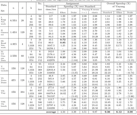
Table 2.1Time and speedup on an Ivybridge machine (16GB memory, 8-core i7-3770K processor)

(“-” indicates that the algorithm fails to run for out of memory)

Data

n d k

No. Assignment Overall Speedup (X) Standard Speedup (X) over Standard of Yinyang

Set iter time/iter

Elkan Drake

Yinyang K-means over

(ms) t= 1 elastic Standard Elkan Drake

I. Kegg Net-work 6.5E4 28 4 16 64 256 50 52 68 59 2.7 9.9 28.0 89.6 1.29 1.62 1.78 1.89 1.97 2.13 2.21 1.63 2.08 2.48 2.55 2.23 2.08 2.48 3.37 4.98 1.14 1.61 2.61 4.86 1.09 1.36 1.98 3.60 1.07 1.12 1.56 3.98 II. Gassen-sor 1.4E4 129 4 16 64 256 16 54 66 55 3.1 5.4 20.3 84.3 4.60 2.84 5.08 6.48 4.34 2.01 3.08 2.06 4.68 2.70 3.17 3.01 4.68 2.70 5.49 10.28 1.13 1.41 3.29 5.40 1.07 1.07 1.82 1.85 1.11 1.27 2.28 4.72 III. Road Net-work 4.3E5 4 4 64 1,024 1E4 24 154 161 74 10.1 80.0 1647.3 16256.1 0.72 0.85 1.25 -1.23 3.42 2.14 1.88 1.36 4.10 4.08 2.80 1.36 3.85 8.45 9.63 1.18 3.63 13.59 12.57 1.24 3.82 12.71 -1.17 1.12 5.21 6.84 IV. US Cen-sus Data 2.5E6 68 4 64 1,024 1E4 6 56 154 152 182.0 2176.4 37603.9 432976 1.88 3.57 0.23 -1.94 4.56 2.96 - (1.64) 2.08 4.85 3.56 2.90 2.08 8.47 24.89 3.05 1.10 5.40 23.45 5.70 1.04 2.43 89.53 -1.04 2.14 6.33 - (2.15) V. Cal-tech101 1E6 128 4 64 1,024 1E4 55 314 369 129 111.0 1432.6 22816.8 316850 2.44 5.52 5.56 -2.88 5.07 3.62 - (3.25) 3.02 5.64 3.38 3.12 3.02 10.21 21.99 20.24 1.83 8.65 22.33 22.23 1.41 1.79 6.41 -1.04 1.26 5.71 - (6.74) VI. Notre Dame 4E5 128 4 64 1,024 1E4 145 232 149 47 46.8 585.8 9334.1 126815 2.85 5.27 5.66 -3.38 4.57 2.82 2.35 3.69 4.29 2.28 2.32 3.69 6.81 10.44 10.81 2.40 6.16 10.69 11.53 1.65 1.88 3.25 -1.05 1.76 4.19 5.27 VII.

Tiny 1E6 384

4 64 1,024 1E4 103 837 488 146 277.0 4113.4 64078.8 781537 6.67 14.23 16.02 -7.58 7.39 4.37 - (3.45) 8.20 6.32 2.94 2.35 8.20 15.26 23.64 15.51 3.24 13.89 23.21 16.13 1.90 1.93 2.78 -1.21 1.93 5.14 - (5.96) VIII.

Uk-bench 1E6 128

4 64 1,024 1E4 62 506 517 208 113.7 1431.1 22787.4 316299 2.63 5.75 5.95 -2.86 7.36 4.28 - (3.92) 3.17 6.61 3.42 3.09 3.17 13.21 23.41 28.50 1.94 10.85 24.26 32.18 1.46 3.12 6.85 -1.10 1.72 5.18 - (6.32)

(29)

Table 2.2Overall speedup over standard K-means on a Core2 machine (4GB mem, 4-core Core2 CPU)

(*: not a meaningful setting for the small data size; -: out of memory)

Data Set I II III IV V VI VIII

k=4 Yinyang 1.35 1.10 1.09 1.13 1.97 2.60 2.05

Elkan 1.09 1.08 0.90 1.06 1.30 1.44 1.32

Drake 1.26 1.05 1.05 1.08 1.79 2.44 1.82

k=64 Yinyang 2.34 2.91 2.79 5.23 8.12 5.75 10.39

Elkan 1.33 2.29 0.97 2.25 3.52 3.23 3.43

Drake 2.04 1.67 2.31 4.42 3.17 2.96 3.28

k=1024 Yinyang * * 8.98 20.41 22.64 10.64 27.34

Elkan * * 1.20 – – 3.52 –

Drake * * 2.18 – (3.18) 3.26 2.48 3.79

k=10,000 Yinyang * * 14.74 6.39 17.87 8.20 28.11

Elkan * * – – – – –

Drake * * – (2.01) – (1.68) – (2.58) – (1.73) – (3.02)

value oft except for the two small ones (100 for data set IV and 500 for others) so that all its executions fit in memory. Table 2.2 does not show data set VII because it cannot fit in memory even in the case of the standard K-means on that machine.

Elkan’s algorithm, which directly keeps k local lower bounds for each point, is still one of the fastest known exact K-means. In comparison, our results show that Yinyang K-means gives consistent and significant speedup. The consistency manifest in three aspects. First, unlike Elkan’s algorithm which often fails (marked with “-”) for running out of memory when k is large due to its n_⇤k space overhead, Yinyang K-means scales withk and shows even greater speedup for larger k values. Second, when the amount of available memory becomes smaller as Table 2.2 shows, Yinyang K-means still produces substantial speedups on all data sets and

k values thanks to its elastic control of t, while Elkan’s algorithm fails to run in even more cases. Finally, whendis small as in the third data set, Elkan’s algorithm runs slower than the standard K-means. It is because to detect an unnecessary distance calculation, in most cases, Elkan’s algorithm requires 6_⇤kcondition checks per point, the time overhead incurred by which is even comparable to the distance calculations on that point. The more e↵ective group filter in Yinyang K-means ensures that for most points, onlytcondition checks are sufficient per point, and hence gives up to 15X speedups for that data set.

Drake’s algorithm maintains one upper bound and t lower bounds: t 1 lower bounds for the first t 1 closest centers, and one for all other centers. As they mentioned in the paper [DH12a], this design can beat Elkan’s algorithm in the intermediate dimension 20< d <

(30)

grouping-based filter makes it less sensitive to “big movers”, its local filter helps further avoid distance calculations, and its elasticity makes it better adapt to space constraints. Drake’s algorithm sets t to k/4 and gradually reduces it to k/8. It fails to run on the large data sets when k is large as the “-” shows in Tables 2.1 and 2.2. We managed to extend the algorithm with our elastic scheme (reducing t to fit memory constraint) to make the algorithm work. The results are shown in parentheses in Tables 2.1 and 2.2. Even with the extension, Yinyang K-means is still over 3X faster than Drake’s algorithm on average.

The carefully designed group filtering of Yinyang K-means contributes substantially to the speedup. As Table 2.3 shows, the filter consistently outperforms the filters in both Elkan’s and Drake’s algorithms. It avoids 80% of distance calculations on average; in comparison, Elkan’s and Drake’s algorithms avoid 13% and 68% respectively. Its local filtering gives it a further edge over Drake’s algorithm.

Table 2.3Unnecessary distance calculations detected by the non-local filters of Yinyang K-means, Elkan’s algorithm, and Drake’s algorithm. (k= 64)

Data Set I II III IV V VI VII VIII average

Yinyang 69.3% 71.0% 88.5% 85.1% 81.7% 77.9% 82.0% 86.2% 80.2%

Elkan 31.1% 32.5% 32.6% 9.2% 0.5 % 2.0E-6 1.6E-6 1.4% 13.4%

Drake 64.2% 58.6% 69.3% 71.7% 73.6 % 68.1% 62.9% 77.7% 68.3%

Another algorithm based on triangle inequality is by Hamerly and others [Ham10a]. It only maintains one lower bound and one upper bound across iterations. It has no group filtering, local filtering, or optimization of center update. Its performance is similar to our global filtering, and more than 3 times lower than our algorithm.

(31)

Table 2.4Yinyang K-means accelerates the center update step by many times

(*: not a meaningful setting for the small data size)

Data Set I II III IV V VI VII VIII

k=4 2.4 3.2 2.1 1.8 4.1 4.3 9.0 4.0

k=64 9.6 20.1 8.4 8.0 11.0 9.8 15.4 11.9

k=1024 * * 107.0 59.9 97.0 43.1 106.6 114.3

k=10,000 * * 62.5 79.7 66.2 27.5 50.8 100.4

Approximation-based algorithms could be used in cases where the clustering quality is not crit-ical, while Yinyang K-means can be used in all scenarios where the standard K-means applies. Being able to give the same results as the standard K-means gives but in only a small fraction of its time is powerful: The great number of practical uses of the standard algorithm can directly adopt our algorithm without worrying about any changes in the output. It naturally inherits the trust that the Lloyd’s algorithm has established among users through decades of usage.

2.5.2 Speedup on the Center Update Step

K-means is a two-step iterative algorithm. As time complexity of the center update step is less than that of theassignment step, prior work focuses only on improving theassignmentstep. But with that step optimized, theupdate step starts to appear prominent in time. Table 2.4 reports the speedup obtained by the optimization described in Section 2.3.2. The speedup ranges from 1.8X to over 100X; substantial speedup show up whenkis large because the time cost of center update calculation, instead of the launching process itself, becomes prominent.

2.5.3 Overall Speedup

The rightmost three columns in Table 2.1 report the overall speedup of Yinyang K-means over the standard K-means, Elkan’s algorithm and Drake’s algorithm, in terms of end-to-end execution time. Yinyang K-means is the fastest in all cases. It is an order of magnitude faster than the standard K-means in most cases, and several times faster than Elkan’s and Drake’s algorithms.

2.5.4 Sensitivity Study on t

(32)

1 4 16 64 256 1024 0

4000 8000

12000 k=1,024

Caltech 101 NotreDame Tiny Ukbench

t

C

P

U

t

im

es

(

m

s/

ite

r)

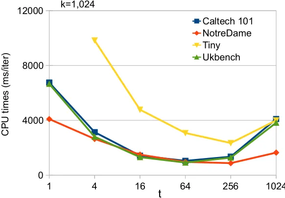
Figure 2.2 Averaged CPU times of assignment step for Yinyang K-means as a function oft.

Figure 2.2 shows the averaged assignment times for Yinyang K-means as a function of t. For legibility, it includes the results on the four image data sets only; similar results show on other data sets. As t increases, the performance of Yinyang K-means first improves and then reaches optimal aroundt=k/10 after which performance decreases. This is because although increasingtproduces tighter lower bounds which help eliminate redundant distance calculations, it incurs more comparison operations and more lower bound updates, which at some point adversely impact performance. The observation led to the design of the aforementioned policy on selecting the value for t in Yinyang K-means. It is worth mentioning that even whent is 1 (when the group filter reduces to global filter), Yinyang K-means still consistently outperforms the standard K-means on all data sets in all settings, as shown by the “t=1” column in Table 2.1, which demonstrates the benefits of the new way to approximate the overlapped Voronoi areas. Overall, the experiments confirm that Yinyang K-means is consistently faster than both the standard K-means, Elkan’s and Drake’s algorithms, regardless of the dimension and size of the data sets, the number of clusters, and the machine configurations. It accelerates both theassignment and center update steps in K-means, and automatically strikes a good tradeo↵ between space cost and performance enhancement.

(33)

practical replacement of the standard K-means as long as triangle inequality holds. The source code of the work in this chapter is available at

http://research.csc.ncsu.edu/nc-caps/yykmeans.tar.bz2.

2.6 Related Work

The work closest to ours includes the K-means optimized by Elkan [Elk03a] and by Drake and Hamerly [DH12a]. They also use triangle inequality to avoid some distance calculations, but di↵er from our algorithm in some critical aspects. Compared to Elkan, our algorithm shows great advantages in the efficiency of the non-local filter (group/global filter). Figure 2.3 shows that intuitively. Figures 2.3 (a) and (b) depict the Voronoi diagrams1 in two consecutive iterations of K-means. It is easy to see that if a point (e.g., the “x”) is in the grey area in Figure 2.3 (b), its cluster assignment needs no update in iterationj+1. Elkan’s algorithm tries to approximate the overlapped Voronoi areas with spheres as the disk in Figure 2.3 (c) shows. The radius of the sphere is half of the shortest distance from the center to all other centers. In contrast, the lower and upper bounds maintained at each point make Yinyang K-means approximate the overlapped areas much better, and hence more e↵ective in avoiding unnecessary distance calculations. Our experiments show that the group filter in Yinyang K-means helps avoid at least two times (over 6X in most cases) more distance calculations than the non-local filter in Elkan’s algorithm as shown in Table 2.3.

x

c

c’

x

c

by Elkan’s alg.

by our alg.

(a) iteration i (b) iteration i+1 (c) approx. of overlapped areas

: boundary of Voronoi cells in iteration i : boundary of Voronoi cells in iteration i+1 : center in iteration i : center in iteration i+1 : a point to cluster

Figure 2.3 The Voronoi diagrams in two consecutive iterations ofk-means, and the approximation of the overlapped areas by our algorithm (t= 1) and Elkan’s algorithm.

(34)

Elkan’s algorithm mitigate the inefficiency through a local filter, which however requires k

lower bounds for each point and a series of condition checks, entailing large space and time cost. As Table 2.5 shows, Elkan’s algorithm takesO(n_⇤k) space and time to maintain lower bounds, while Yinyang K-means takes onlyO(n⇤t). The non-local filtering time cost isO(k2⇤d+n) for Elkan’s algorithm, andO(n)_⇠O(n_⇤t) for Yinyang K-means, depending on whether the global filter works. The two methods have a similar local filtering time complexity,O(n_⇤↵_⇤k), with↵ for the fraction of points passing through the non-local filter. However, as shown in Table 2.3,↵ is much smaller in Yinyang K-means than in Elkan’s algorithm (0.2 vs. 0.86 on average), thanks to the more powerful non-local filter of Yinyang K-means. The cost causes Elkan’s algorithm to fail or perform inferiorly in some scenarios, as shown in the next section.

Drake’s algorithm tries to lower the time and space cost of the local filter of Elkan’s algo-rithm. For each point, it maintains tlower bounds, with the first (t 1) for the distance from the point to each of its (t 1) closest centers, and the tth for all other centers. As Table 2.5 shows, its time and space costs are lower than Elkan’s algorithm (but still higher than Yinyang K-means). It is however still sensitive to “big movers”, because the update of the tth lower bound uses the maximal drift, and the impact propagates to other lower bounds due to the order of lower bounds that the algorithm needs to maintain.

In comparison, the grouping-based filter design of Yinyang K-means mitigates the sensitivity to “big movers”. It, along with the elasticity, helps Yinyang K-means excel over the prior algorithms. In addition, Yinyang K-means is the only algorithm that optimizes not only the assignment step but also the centerupdate step of K-means. quantitative comparisons next.

Table 2.5Cost Comparison (n: # points;k: # clusters;t: # lower bounds per point;↵: fraction of points passing through the non-local filter; Drake’s algorithm has no local filter)

Algorithm space cost time cost

lower bounds maintenance non-local filtering local filtering Yinyang K-means O(n⇤t) O(n⇤t) O(n)⇠O(n⇤t) O(n⇤↵⇤k)

Elkan’s [Elk03a] O(n_⇤k) O(n_⇤k) O(k2

(35)

CHAPTER

3 AUTOMATIC ALGORITHMIC

OPTIMIZATIONS FOR

DISTANCE-RELATED PROBLEM

In this chapter, we presents Triangular OPtimizer(TOP), the first compiler-based framework that is able to automatically produce optimized algorithms for distance-related problems (this work [Din15a] has been published in VLDB 2015).

3.1 Problem Statement

In this chapter, we describe two example problems that involve distance calculations and point out some unnecessary distance calculations in them. The conveyed intuition will help understand the following discussions on the design of the proposed software framework.

(36)

q c1

c’1

c2

c’2

(a) KMeans _{(b) P2P}

q

t

Figure 3.1 Example distance problems.

distances between every point and every center in order to find the center closest to each point. Some of the calculations are unnecessary. Consider Figure 3.1 (a), where, c0₁ is the center of pointqin the previous iteration andc0₁gets updated intoc1 at the end of the previous iteration;

c0₂ andc2are the centers of another cluster in the two iterations. If we can quickly get the upper bound of the distance betweenqandc1, denoted asd(q, c1), and the lower bound ofd(q, c2), we may compare them first. If the former is smaller than the latter, we can immediately conclude thatc2 is impossible to be the new center forx and avoid computing d(q, c2).

Point-to-point shortest path problem (P2P), illustrated in Figure 3.1 (b), is another example. It tries to find the shortest path between two points in a directed graph. The length of each edge in the graph is known. Distance in this problem is defined on a 3-tuple (two points and a path between them), meaning the length of that path between the two points. During the search for the shortest path among all paths between a query point (q) and a target point (t), we can avoid computing the full length of a path if we can quickly determine that the lower bound of its length is greater than the length of the shortest path encountered so far.

3.2 Overview of Proposed Solution

TOP unifies many algorithms across these domains through a generic distance-related abstrac-tion. Based on this abstraction, it derives seven principles for correctly applying the triangular inequality to optimize distance-related algorithms. The result shows that top is able to auto-matically produce optimized algorithms that either matches or outperforms manually designed algorithms for solving distance-related problems.

(37)

/*

Goal: Cluster points in S into K classes with T containing all cluster centers. S: a set of query points to cluster.

T: a set of target points (i.e., cluster centers). N: a set of indices of points. |N|=|S|.

*/

… // declarations

TOP_defDistance(Euclidean); // distance deﬁnition

T = init();

changedFlag = 1; while (changedFlag){

// ﬁnd the closest target (a point in T) for each point in S

N = TOP_ﬁndClosestTargets(1, S, T);

TOP_update(T, &changedFlag, N, S); // T gets updated

}

Figure 3.2 K-Means written in TOP API (detailed in Chapter 3.5). Prefix “TOP ” indicates calls to TOP API. They will be replaced with low-level function calls by TOP compiler, making the algorithm automatically avoid unnecessary distance calculations.

distance-based calculations that meet the Triangular Inequality condition (see Chapter 3.4.1), regardless of the domain, definition of distances, distance calculation patterns, usage of the distances, and so on. Its generated algorithm matches or outperforms the algorithms manually designed by the domain experts. With TOP, decades of manual e↵ort by domain experts could have been saved; it makes optimizing new distance-based problems much easier, and boost the performance of existing algorithms.

Specifically, we propose a simple abstraction, called abstract distance-related problem, to formalize various distance-related algorithms across seemingly disparate domains, in a unified manner. The abstraction allows a systematic examination of all kinds of scenarios related with distance computations, which in turn, leads to a spectrum of algorithmic optimization along with some automatic mechanisms for selecting the best optimization to use. We turn all these findings into a runtime library, the invocations of which in a program would automatically save unnecessary distance calculations for an arbitrary distance-related problem (that meets the triangular inequality condition).

Along with the library, we equip TOP with a set of APIs and a compilation module. Through the API, programmers can easily specify the distance problem, as illustrated in Figure 3.2. The compiler module then derives important properties of the problem, and inserts necessary calls of the library such that at runtime, unnecessary distance calculations can be e↵ectively detected and avoided.

(38)

on average) the state-of-the-art algorithms that have been designed by domain experts. It is able to generate new algorithms for problems, on which no prior work has applied triangular inequality optimizations, and achieves 237X speedups.

Overall, the work in this chapter makes the following contributions:

• Abstraction:It o↵ers an abstraction that unifies various distance-related problems, which lays the foundation for the development of automatic optimizing frameworks.

• Algorithmic Optimization: It develops the first set of principled analysis on how triangu-lar inequality should be applied to a spectrum of distance-related problems, reduces the algorithmic optimizations into two key design questions (landmark selection and compar-ison ordering), reveals a strand of insights, and crystallizes them into seven principles in enabling e↵ective distance-related optimizations.

• TOP Framework: It builds the first software framework that can automatically apply algorithmic optimization on various kinds of distance-related problems.

• Results:It shows that the automatic framework can yield algorithms that match or out-perform manually designed ones. Some of the algorithms have never been proposed for the distance-related problems by domain experts.

To develop a unifying software framework for addressing the various distance-related prob-lems, there are three steps:

(1) Come up with an abstraction to represent the various problems in a unified manner; (2) Based on the unifying abstraction, systematically examine the optimizations that have been manually applied to the various distance-related problems. Through the examination, uncover the essence of distance optimizations and find out the principles for applying them e↵ectively.

(3) Develop the necessary API, compiler support, and runtime libraries to integrate all the findings and insights into a software framework, which can then automatically apply the opti-mizations to any problem of that class.

To the best of our knowledge, there is no prior work on any of the three steps. They hence all need some innovations and substantial work to develop; the second step turns out to be particularly challenging in our exploration.

(39)

3.3 Unifying Abstraction

Although both involve distance calculations, the two examples described in the previous chapter di↵er in many aspects, including their domains (data mining versus graph analysis), nature of problem (iteratively putting points into groups versus finding a path in a graph), distance definitions, and constraints of distance calculations (subject to graph connectivity or not). It is hence not a large surprise that even though both problems involve unnecessary distance calculations, no research has tried to find commonalities in the two problems and provide a general solution for them or other distance-related problems. We find many papers published on optimizations specific to each of the two problems for avoiding unnecessary distance calculations ([Elk03b; DH12b] for K-Means, [GH05; Gut04] for P2P). We also find such problem-specific manual e↵orts in many other distance-related problems, even for some problems residing in the same domain (e.g., K-Means [Elk03b; DH12b] and KNN [Wan11; Gre00]).

Despite the di↵erences among these problems, they are all related with distance calcula-tions. A key view motivating this study is that if we can have an abstraction to represent all such distance-related problems, we may be able to derive a general approach to optimizing algorithms for such problems at that abstraction level.

Abstraction. We introduce the notion ofabstract distance-related problemas follows: It is an abstract form of the problems that aim at finding some kind of relations between two sets of points, a query set and a target set; the relations are about a certain type of distances defined between the two sets of points under a certain set of constraints. We denote such a problem with a five-element tuple (Q, T, D, C, R):

• Q: the query set of points. It may contain one or more points in a space. It is the central entity of the relations of interest.

• T: the target set of points. It is the other party of the relations of interest.

• D: a type of distance between points.

• C: constraints related with the problem. They can be about the connectivity between Q and T, available memory in the system, or some other conditions. A special condition is whether the distance problem of interest involves many iterations of update on Q or T. If so, we call the problem an iterative distance problem.

(40)

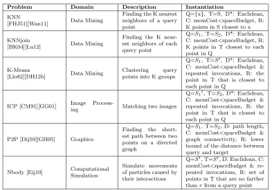
Table 3.1Six Important Distance-Related Problems.

Problem Domain Description Instantiation

KNN

[FHJ51][Wan11] Data Mining

Finding the K nearest neighbors of a query point

Q={x}, T=S, D*: Euclidean, C: memCost<spaceBudget, R: K points in S closest to x

KNNjoin

[BK04][Lu12] Data Mining

Finding the K near-est neighbors of each query point

Q=S1, T=S2, D*: Euclidean,

C: memCost<spaceBudget, R: K points in T closest to each point in Q

K-Means

[Llo82][DH12b] Data Mining

Clustering query points into K groups

Q=S1, T=St, D*: Euclidean,

C: memCost<spaceBudget & repeated invocations, R: the point in T that is closest to each point in Q

ICP [CM91][GG01] Image

Process-ing Matching two images

Q=S1t, T=S2, D*: Euclidean,

C: memCost<spaceBudget & repeated invocations, R: the point in T that is closest to each point in Q

P2P [Dij59][GH05] Graphics

Finding the short-est path between two points on a directed graph

Q=S1, T=S2, D: path length,

C: memCost<spaceBudget & graph connectivity, R: lower bound of the distance between query and target

Nbody [Eij10] Computational Simulation

Simulate movements of particles caused by their interactions

Q=St_{, T=}_St_{, D: Euclidean, C:}

memCost<spaceBudget & re-peated invocations, R: set of points in T that are no farther thanrfrom a query point

S,S1,S2are all sets of points, which may be identical or di↵erent; superscripttmeans that the set could get

dynamically updated;xis one point; D* could be defined as other types of distance;ris a constant give beforehand.

points, such as the lower bound of the distance, the closest targets to a query point, and so on.

Mappings from the Concrete. The abstraction unifies various distance-related problems into a single form, making automatic algorithmic optimization possible. Table 3.1 presents how six important distance-related problems in various domains can be mapped to the abstraction form. Each of the six problems has been extensively studied in its specific domain, but they have never been treated together in a unified manner. We next explain them and the mappings briefly.

(41)

find the K nearest neighbors for each point in Q.

We have described K-Means in the previous chapter. It maps to our abstraction well. The set of points to cluster is Q, the center set in each iteration is T (the superscript inSt in Table 3.1 stands for iterative update), its constraints include the iterative property and memory limit, and the relation of interest is the closest target for a query point.

ICP is a technique for mapping the pixels in a query image with the pixels in a target image. It is an iterative process. In each iteration, it maps each pixel in a query image with a pixel in the target image that is similar to the query pixel, and then transforms the query image in a certain way.

As aforementioned, P2P is a graphic problem that tries to find the shortest path between two points (one in Q, the other in T) in a directed graph. Q and T are two sets of points on that graph. The distance of interest is about the path between points, and is hence subject to the connectivity among vertices in the graph. The relation of interest is the lower bound of the path length between two points.

Many algorithms have been manually designed specifically for each of the five problems for avoiding unnecessary computations: KNN [Wan11; Gre00; Lai07; Elk07], KNNjoin [Lu12; Yu07; Emr10; Din08; Zha13], KMeans [Elk03b; Ham10b; DH12b; Nga06], ICP [GG01], P2P [GH05; Gut04].

Nbody [Eij10] simulates the interplay and movements of particles in a series of time steps. In each step, it computes the distances between every particle and all particles in its neighborhood in every time step, from which, it derives the force that particle is subject to, computes its movement accordingly, and updates its position. The algorithm has some variations. The one used in the work in this chapter defines the neighborhood of a particle as a sphere of a given radius. The Q and T in this problem are identical, referring to the set of particles.

3.4 Principles of Distance Optimizations

(42)

c

a

b

|d(a,b) - d(b,c)| d(a,c) d(a,b) + d(b,c)

Figure 3.3 Illustration of distance bounds obtained from Triangular Inequality (bis a landmark).

After that, we present seven principles we attain for using triangular inequality for e↵ective optimizations, which serve as the foundation for our automatic optimization framework TOP.

3.4.1 Triangular Inequality (TI): Concepts and Implications We give the formal definition of TI as follows:

Leta, b, crepresent three points andd(a, b) represent the distance betweenaandb;triangular inequality (TI) states thatd(a, c)_d(a, b) +d(b, c).

Although TI does not hold for all kinds of distances, it holds for many common ones (e.g., Euclidean distance). It provides an easy way to compute both the lower bound and upper bound of the distance between two points as follows. Figure 3.3 gives an illustration.

|d(a, b) d(b, c)|d(a, c)d(a, b) +d(b, c) (3.1)

Formula 3.1 o↵ers the fundamental connection between TI and distance-related problems. Intuitively, if the lower or upper bound of the distance between two points could be used in place of their exact distance in solving a distance-related problem, the bounds provided by Formula 3.1 may save the calculation of their exact distance.

But how using the bounds could help may not be immediately clear. As the formula shows, to get either the upper or lower bound of the distance between two points “a” and “c” in order to save the calculation ofd(a, c), we need two distancesd(a, b) andd(b, c). So at the first glance, there seems to be no benefit but extra cost to use the bounds. However, when we consider the context of distance-related problems, the benefits become easy to see. It relates with the following two concepts we introduce.