University of Windsor University of Windsor
Scholarship at UWindsor
Scholarship at UWindsor
Electronic Theses and Dissertations Theses, Dissertations, and Major Papers
1-1-2007
A statistic approach of multi-factor sensitivity analysis for
A statistic approach of multi-factor sensitivity analysis for
service-oriented software systems.
oriented software systems.
Chunjiao Ji
University of Windsor
Follow this and additional works at: https://scholar.uwindsor.ca/etd
Recommended Citation Recommended Citation
Ji, Chunjiao, "A statistic approach of multi-factor sensitivity analysis for service-oriented software systems." (2007). Electronic Theses and Dissertations. 7132.
https://scholar.uwindsor.ca/etd/7132
NOTE TO USERS
This reproduction is the best copy available.
®
A Statistic Approach of Multi-factor Sensitivity
Analysis for Service-oriented Software Systems
by
Chunjiao Ji
A Thesis
Submitted to the Faculty o f Graduate Studies and Research
through Computer Science
in Partial Fulfillment o f the Requirements for
the Degree o f Master o f Science at the
University o f Windsor
Windsor, Ontario, Canada
2007
1*1
Library and Archives CanadaPublished Heritage Branch
395 Wellington Street Ottawa ON K1A0N4 Canada
Bibliotheque et Archives Canada
Direction du
Patrimoine de I'edition
395, rue Wellington Ottawa ON K1A0N4 Canada
Your file Votre reference ISBN: 978-0-494-42323-3 Our file Notre reference ISBN: 978-0-494-42323-3
NOTICE:
The author has granted a non exclusive license allowing Library and Archives Canada to reproduce, publish, archive, preserve, conserve, communicate to the public by
telecommunication or on the Internet, loan, distribute and sell theses
worldwide, for commercial or non commercial purposes, in microform, paper, electronic and/or any other formats.
AVIS:
L'auteur a accorde une licence non exclusive permettant a la Bibliotheque et Archives Canada de reproduire, publier, archiver,
sauvegarder, conserver, transmettre au public par telecommunication ou par Nntemet, preter, distribuer et vendre des theses partout dans le monde, a des fins commerciales ou autres, sur support microforme, papier, electronique et/ou autres formats.
The author retains copyright ownership and moral rights in this thesis. Neither the thesis nor substantial extracts from it may be printed or otherwise reproduced without the author's permission.
L'auteur conserve la propriete du droit d'auteur et des droits moraux qui protege cette these. Ni la these ni des extraits substantiels de celle-ci ne doivent etre imprimes ou autrement reproduits sans son autorisation.
In compliance with the Canadian Privacy Act some supporting forms may have been removed from this thesis.
While these forms may be included in the document page count,
their removal does not represent any loss of content from the thesis.
Conformement a la loi canadienne sur la protection de la vie privee, quelques formulaires secondaires ont ete enleves de cette these.
Bien que ces formulaires
Abstract
The performance aspect of a service-oriented system is of paramount
importance. As system architecture determines the quality of software systems,
performance effects of architectural decisions can be evaluated at an early stage
by constructing and analyzing quantitative performance models that capture the
interactions between the main components of the system as well as the
performance attributes of the components themselves. But accurate
performance analysis results need sensitivity analysis be taken into account.
This thesis proposes and implements a statistic approach of multi-factor in
sensitivity analysis. It carries out a quantitative sensitivity analysis of
service-oriented system with better accurateness due to considering more factors as
input and simultaneously, got multi-pairs of interactions between factors. Also
two different methods of optimizing the software architectural design of a web
DEDICATED
To my parents, my family, my sisters, brothers,
Acknowledgements
I am very grateful to my supervisor, Professor Xiaobu Yuan, for his invaluable
guidance, constant encouragement and patience throughout the research period.
I feel lucky that he supervised my thesis. I would also like to thank my thesis
committee members, Dr. Jianwen Yang, Dr. Joan Morrissey and Dr. Arutina
Jaekel, who have been all generous and patient. Their confidence in my abilities
has been unwavering, and has helped to make this thesis a solid work.
I wish to express my affectionate gratitude to my husband Caishi Wang, my mom
Yulan Liu, my parents-in-law Junda Wang and Shuying Jiao, my sisters Fengjiao
and Sanjiao, for their love and support, for never doubting in me, always being
proud of me and never letting me forget it. Without their encouragement and
support, I would not go this far. Their love is one of the most important parts in
my life. Deep appreciation also goes to other relatives and close friends who
encourage me to make great dreams come to true, though I cannot list their
CONTENTS
ABSTRACT... Ill
DEDICATION...IV
ACKNOWLEDGEMENTS ...V
TABLE OF CONTENTS...VI
LIST OF TABLES...VIII
LIST OF FIGURES... IX
1. INTRODUCTION... 1
1.1 Mo t iv a t io n...2
1.2 Co n t r ib u t io n s... 4
1.3 Or g a n iz a t io n s... 5
2. LITERATURE REVIEW... 6
2.1 Co m p o n e n t-Ba s e d So f t w a r e En g in e e r in g (C B S E )...6
2.1.1 Co m p o n e n t De f in it i o n... 7
2.1.2 Co m p o n e n t-Ba s e d So f t w a r e Lif e Cy c l e (C S L C )... 8
2.2 Se r v ic e-Or ie n t e d So f t w a r e Sy s t e m s... 9
2.2.1 Se r v ic e-Or ie n t e d Ar c h it e c t u r e ( S O A ) ...10
2.2.2 Web-Servtce Ba s e d Sy s t e m s... 12
2.3 So f t w a r e Pe r f o r m a n c e En g in e e r in g (S P E )... 15
2.3.1 Pe r f o r m a n c e Mo d e l s... 16
2.3.2 Pe r f o r m a n c e An a l y s iso f So f t w a r e Ar c h it e c t u r e... 20
2.3.2.1 Pe r f o r m a n c e Ass e s s m e n to f So f t w a r e Ar c h it e c t u r e (P A S A )... 21
2.3.2.2 U M L Pr o f il e f o r Sc h e d u l a b il it y, Pe r f o r m a n c ea n d Tim e (S P T )... 23
2.3.2.3 Pe r f o r m a n c e a n a l y s isw it h t h e An n o t a t e d U M L m o d e l...24
3. A STATISTIC APPROACH... 29
3.1 Pr o b l e m Do m a in... 29
3.3 St a t is t ic Ap p r o a c h...30
3.3.1 Tw o-f a c t o r Fa c t o r ia l Tr e a t m e n t De s ig n...31
3.3.1.1 Tw o-f a c t o r An a l y s is o f Va r ia n c e...34
3.3.1.2 Mu l t ip l e Co m p a r is o n s-S N K Ra n g e Te s t... 37
3.3.2 Mu l t i-f a c t o r Fa c t o r ia l Tr e a t m e n t De s ig n... 40
3.3.2.1 Th r e e-f a c t o r An a l y s is o f Va r ia n c e... 42
4. EXPERIMENTS AND DISCUSSION... 48
4.1 Ex p e r im e n t a l En v ir o n m e n t Ov e r v ie w... 48
4.2 Ex p e r im e n t s...49
4.2.1 Da t a c o l l e c t in ga n d q u a n t it a t iv ea n a l y s is...52
4.2.1.1 Case 1 ...52
4.2.1.2 Co m p a r in gt o Tw o-f a c t o r Fa c t o r ia l Tr e a t m e n t De s ig n...58
4.2.1.3 Ca se 2 ... 60
5. CONCLUSIONS AND FUTURE WORK... 66
5.1 Co n t r ib u t io no ft h e Re s e a r c h...66
5.2 Dir e c t io n so f Fu t u r e Wo r k... 67
BIBLIOGRAPHY... 69
LIST OF TABLES
Table 3.1 Pressure Inside a Vacuum Tube...32
Table 3.2 Formulized Table Pressure Inside a Vacuum Tube... 33
Table 3.3 The Analysis of Variance Table for Two-Factor Factorial Treatment Design... 36
Table 3.4 Analysis of Variance for Vacuum Tube Pressure Experiment... 37
Table 3.5 Data for Power Requirement...41
Table 3.6 Formulized Table for Power Requirement... 42
Table 3.7 The Analysis of Variance Table for Three-Factor Factorial Treatment Design... 46
Table 3.8 Analysis of Variance for Power Requirement... 47
Table 4.1 System Response Time(s) for Case 1 ... 53
Table 4.2 Analysis bf Variance for Case 1 ...53
Table 4.3 Data for B=0.5... 58
Table 4.4 Analysis of Variance for Table 4 .3 ... 58
Table 4.5 Data for B = 1 ... 59
Table 4.6 Analysis of Variance for Table 4 .5 ... 59
Table 4.7 Data for B = 2 ... 60
Table 4.8 Analysis of Variance for Table 4 .7 ...60
Table 4.9 System Response Time(s) for Case 2 ... 61
LIST OF FIGURES
Figure 2.1 Service-Oriented Architecture...10
Figure 2.2 Web Service Architecture...14
Figure 2.3 Basic Service Description...15
Figure 2.4: Interface in U M L... 15
Figure 2.5: Typical queuing network...17
Figure 2.6 An example of simple LQN model... 18
Figure 2.7 A simple sequence diagram...25
Figure 2.8Layered system example of a web-based ticket reservation system...27
Figure 4.2 Annotated UML Sequence Diagram for Web Services Invocation 51 Figure 4.3 Layered Queuing Network Model for Web Services Invocation...52
1. Introduction
Since the naissance of the first computer, software industry has been searching
for effective techniques to deal with the difficulties of software development. In
the past decades, the complexity of software systems has increased dramatically,
and productivity and time-to-market become the major concerns of software
industry. Traditional approaches of software development failed to cope with
sophisticated applications of computer systems. In comparison,
Component-Based Development (CBD) allows software systems to be developed from pre
produced parts, thus improving not only productivity but also the quality and
maintainability of software products. In CBD, pre-produced parts can be easily
maintained and customized to produce new functions and features for them to be
reused in different applications [HC01]. CBD promises increased productivity and
reduced development efforts through larger-grained software reuse [Kim02].
In addition, Service-Oriented Architectures (SOA) has gained a lot of momentum
in software engineering in recent years [TJ05]. As a new technology of dealing
with the challenge of interoperability of systems in heterogeneous environments,
SOA helps IT organizations to support alignment with business requirements that
are changing at an increasing rate. Other benefits of SOA include reuse of
components, improved reliability, and reduced development and deployment
costs [KKL+05]. A service-oriented architecture consists of a collection of
services that communicate with each other [TJ05]. It must also provide the
mechanism to support the functionality for service description and publishing,
service discovery, and service consumption/interaction. When services use the
Internet for the means of communication, the inter-service infrastructure
becomes web services-based. Component-Based Development provides a tried
The remaining of this chapter first introduces performance analysis of SOA and
web services-based systems as the motivation of the proposed thesis research.
Afterwards, contributions of this thesis research are explained with highlights of
sensitivity analysis for service-oriented software systems. The structure of the
thesis proposal is also given in the section of organizations.
1.1 Motivation
As a key factor that determines the success of software development, software
performance is considered extremely important in the practice of
component-based and web service-component-based software systems [BJK02]. The performance
aspect of a service-oriented system is of paramount importance. While SOA has
gained its popularity, the actual performance of SOA systems is still
unpredictable. As system architecture determines the quality of software systems,
performance effects of architectural decisions can be evaluated at an early stage
by constructing and analyzing quantitative performance models that capture the
interactions between the main components of the system as well as the
performance attributes of the components themselves. It is more cost-effective to
push performance analysis back to a very early stage of architectural design.
J
Typical performance analysis of software architectures involves three steps
[PS02]: firstly, the UML (Unified Modeling Language) model of the software
architecture is translated into a performance model, such as Queuing Network
model (QN) [Buz71], Layered Queuing Network model (LQN) [RS95], and
Stochastic Rendezvous Network model (SRVN) [WNP95]. In the second step, a
performance analysis tool, such as the LQN solver, conducts experiments on the
performance model. Finally, the experiment results are fed back into the UML
Before the experiment results are fed back into the UML model, the studying of
sensitivity of performance of systems due to the effects of system factors are
very important.
Unfortunately, The sensitivity analysis for service-oriented software systems
does not catch enough attention. Much of the software industry’s focus is
currently on the underlying technology for the design, implementation, and
application of Web services and their interactions [ABG+01] [MMF02] [HL03]
[GH02] [GDH05] [LGH05]. How can we design a system to meet the
performance requirement while take advantage of service-oriented architecture?
There is a growing body of research that studies performance analysis. In [AG97]
[SG96], the authors focus on the studies of the role of software architecture in
determining different quality characteristics in general, while in [SG98] [WS98],
authors focus on performance characteristics in special. In [LK98] [GT02] [GT01]
the robustness and reliability of analysis methods are discussed. But accurate
performance analysis results need sensitivity analysis be taken into account. V.S.
Sharma and K.S. Trivedi introduced security and cache behavior into architecture
reliability analysis as an effort to produce accurate analysis results [ST05].
However, none of the above quantitatively takes into account the interaction
between factors that effects system performance.
In [KL98] a statistic technique is used for performance analysis to reduce
perturbation and data volume while retaining interesting characteristics of
performance data. A statistical framework for analyzing the performance
sensitivity of designs to various timing related effects, noise and variations are
proposed in [LKC+00]. But Statistic method used on performance analysis for
As described above, there are three steps in performance analysis. Between
step 2 and step 3, studying the sensitivity of performance of a system due to the
effect of system factors is very important. However, little research has been done
in service-oriented software systems. In [Hua04], the author did an effort to
consider interactions. But it took into account only two factors and one
observation per treatment condition, where there is not a clear-cut way to
separate the effect of the interaction of the two factors from the experimental
error [LM74], its further discussion based on that there is no interaction between
factors. So a more accurate approach, multi-factor sensitivity analysis approach
with multi-observation per cell, is proposed.
1.2 Contributions
Sensitivity analysis that replies upon human sense on graphical analysis to
decide the quality of architecture designs unavoidably reduces the quality of
analysis results. This thesis applies a statistic approach of multi - factor in
sensitivity analysis. It provides a quantitative sensitivity analysis of
service-oriented system. In regard to two factors approach, it has better accurateness
due to considering more factors as input and simultaneously, got multi-pairs of
interactions between factors, not only one pair between two factors. Also two
different methods of optimizing the software architectural design of a web
service-based system are developed, one is based on having interactions and
the other for no interaction. Introducing multi-factors sensitivity analysis in
performance analysis in early design stage will lead to robust architecture design
because it produces more accurate quantitative feedback to software designers,
and help them to optimize the development of sen/ice-oriented software systems.
No doubt it helps to reduce the cost of software development and improve quality
1.3 Organizations
In the following part of this thesis, the background of all the related fields, i.e.
component-based software engineering (CBSE), Service-oriented Software
Systems, Web-service based systems and software performance engineering
(SPE), the analytic model - Layered Queuing Network (LQN) model for
performance evaluation will be introduced. In particular, PASA, a method for
performance assessment of software architecture will be described in detail in
Chapter 2. Chapter 3 presents problem domain, introduces sensitivity analysis
and proposed statistic approach in detail. Chapter 4 describes experiments and
discussions of sensitive analysis based on a service-oriented system - Web
services-based Clinical Decision Support System (CDSS). Finally, the
conclusions, restates the contributions of this thesis and points to future research
2. Literature Review
2.1 Component-Based Software Engineering (CBSE)
In the past decades, as system complexity is increasing sharply, time-to-market
and productivity become key concerns in software industry. Traditional
approaches failed to cope with more sophisticated hardware and software
technologies. Software industries are striving for new techniques and approaches
that could improve software developer productivity, reduce time-to-market,
deliver excellent performance and produce systems that are flexible, scalable,
secure, and robust. Software reuse not only improves productivity but also has a
positive impact on the quality and maintainability of software products.
Component-Based Development (CBD) is an appealing technology that can
meet these demands and following this with providing increased productivity and
reducing development efforts through larger-grained software reuse [Kim02].
And Component-Based Software Engineering (CBSE) has emerged, which has
raised great interest in software industries. CBSE primarily concerns with three
functions [HC01]:
1) Developing software from pre-produced parts
2) The ability to reuse those parts in other applications
3) Easily maintaining and customizing those parts to produce new functions
and features
Component-based software engineering encourages reuse of pre-developed
system pieces rather than building from scratch. It provides managers with
opportunities to streamline their software development process all through its
phases, from analysis to maintenance, and from project planning to project
Although component-based development offers many potential benefits, such as
greater reuse and reduced time-to-market (and hence software production cost).
It also raises several issues that developers need to consider [BBOO] [Lau06]. In
other words, there are still many areas that researchers can work on in this field.
2.1.1
Component Definition
There are still many debates about the definition of component. The following
definitions of software component are commonly cited throughout the literature
[GH03]:
• A component is a language neutral, independently implemented package of
software services, delivered in an encapsulated and replaceable container,
accessed via one or more published interfaces [SpaOO].
• A software component is a coherent package of software artifacts that can be
independently and delivered as a unit and that can be composed, unchanged,
with other components to build something larger. (D’Souza)
• A software component is a physical packaging of executable software with a
well-defined and published interface [HopOO].
• A business component represents the software implementation of an
“autonomous” business concept or business process. It consists of the software
artifacts necessary to express, implement, and deploy the concept as a reusable
element of a larger business system [Koz98].
• A software component is a unit of composition with contractually specified
interfaces and explicit context dependencies only. A software component can be
By analyzing the above definitions of software component, we can derive that a
software component is a coherent package of software implementation; it carries
out a set of related services or functions and offers well-defined and published
interfaces; also it offers services that are accessible through its interfaces only;
finally it is reusable and can be independently developed and delivered.
The software components can be commercially available off the shelf (COTS),
developed in-house, or developed contractually. Modern programs are likely to
be made up of thousands or millions of parts distributed globally, executing
whenever called, and acting as parts of one or more complex systems. Thus,
predicting the performance of an application taking into account sensitivity
analysis is absolutely essential.
2.1.2 Component-Based Software Life Cycle (CSLC)
A typical life cycle of software components consists of the following phases:
design, deployment and run-time [Lau06].
In the design phase, components are constructed, catalogued and stored in a
repository where they can be retrieved later when needed. Components in the
repository can be both source and binary code.
In the deployment phase, components are retrieved from the repository, and
compiled to binary code. These binary components can be composed to a
system that is ready for execution.
In the run-time phase, there is no new composition, but components of a system
CSLC is * the life cycle process for a software component with an emphasis on
business rules, business process modeling, design, construction, continuous
testing, deployment, evolution, and subsequent reuse and maintenance.”[CH01]
Comparing with a traditional software development life cycle, the analysis and
design phases for a CSLC are significantly longer. Much more time is spent in
business rules, business process modeling, analysis and design. Much less time
is devoted to development.
2.2 Service-Oriented Software Systems
In recent times, the use of a service-oriented approach to software engineering
has become popular. Service-Oriented Architectures (SOA) has gained a lot of
momentum in software engineering [TJ05]. Service-Oriented Architectures have
emerged as the main approach for dealing with the challenge of interoperability
of systems in heterogeneous environments, address pressures of IT
organizations to support alignment with business requirements that are changing
at an increasing rate. One aspect of such service-oriented systems is that their
component services can usually be composed and used in a variety of
unplanned-for ways.
When the services use the Internet as the communication mechanism, the inter
service infrastructure becomes web services-based. Component-Based
Development provides a tried and tested foundation for the implementation of a
SOA [BJK02].
2.2.1 Service-Oriented Architecture (SOA)
A web service is “ a software module deployed on network accessible platforms
provided by the service provider.” [CF02] It may be invoked by or to interact with
a service requestor and May also function as a requestor, using other web
services in its implementation.
A Service-Oriented architecture is a collection of services that communicate with
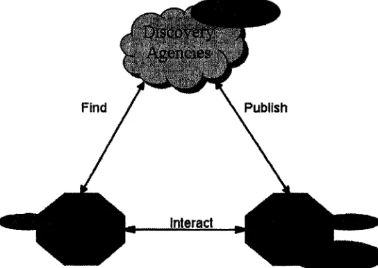
each other. As shown in Fig. 2.1 [CF02], service-oriented architectures involve
three different kinds of actors: service providers, service requesters and
discovery agencies.
Find Publish
Interact
Figure 2.1 Service-Oriented Architecture
• Service requester -- requests the execution of a service. This is the
application that is looking for and invoking or initiating an interaction with a
service. Its role in the client-server message exchange patters is that of a
• Service provider -- processes a service request. It has been referred to as
a service execution environment or a service container. Its role in the
client-server message exchange patterns is that of a server.
• Discovery agency -- agency through which a service description is
published and made discoverable. This is a searchable set of service
descriptions where service providers publish their service descriptions.
The service discovery agency can be centralized or distributed.
The service provider exposes some software functionality as a service to its
clients. Such a service could, e.g., be a SOAP based web service for electronic
business collaborations over the Internet. In order to allow clients to access the
service, the provider also has to publish a description of the service. Since
service provider and service requester usually do not know each other in
advance, the service descriptions are published via specialized discovery
agencies. The discovery agencies work as a “match-maker”. They can categorize
the service descriptions and provide them in response to a query issued by one
of the service requesters. As soon as the service requester finds a suitable
service description for its requirements at the agency, it can start interacting with
the provider and using the service. There are some critical characteristics for
effective use of services recommended by [BJK02]:
o Interface-based design: Services implement separately defined interfaces
o Discoverable: Services need to be found at both design time and run time,
not only by unique identity but also by interface identity and by service
kind.
o Loosely coupled: Services are connected to other services and clients
using standard, dependency-reducing, decoupled message-based
methods such as XML document exchanges.
o Coarse-grained: Operations on services are frequently implemented to
encompass more functionality and operate on larger data sets, compared
o Single instance: Unlike component-based development, which instantiates
components as needed, each service is a single, always running instance
that a number of clients communicate with.
o Asynchronous: In general, services use an asynchronous message
passing approach; however, this is not required.
2.2.2 Web-Service Based Systems
Component-based development makes it possible to assemble an application
from a repository of components developed in various languages by
homogeneous or heterogeneous composition. Web Services provides an easy
way to extend component-based development by adopting open Internet
standards. Web services allow the open and flexible interaction of applications
over the Internet. Web services standards provide a high level of interoperability
across platforms, programming languages and applications. Web services are
invoked over a network, however they do not have to reside on the World Wide
Web; they can be located on an Intranet, or anywhere on the network.
A Web service is “a software system identified by a URI, whose public interfaces
and bindings are defined and described using XML. Its definition can be
discovered by other software systems. These systems may then interact with the
Web service in a manner prescribed by its definition, using XML based
messages conveyed by internet protocols” [CF02]
A software agent in the Web services architecture can act in one or multiple roles,
acting as requester or provider only, both requester and provider, or as requester,
provider, and discovery agency. A service is invoked after the description is
Currently, Web Services technology implements SOA by means of standard
XML-based initiatives. Three initiatives are used in order to support interactions
among Web Sen/ices: SOAP (a way to communicate) [13], W SDL (a way to
describe services) and UDDI (a name and directory server).
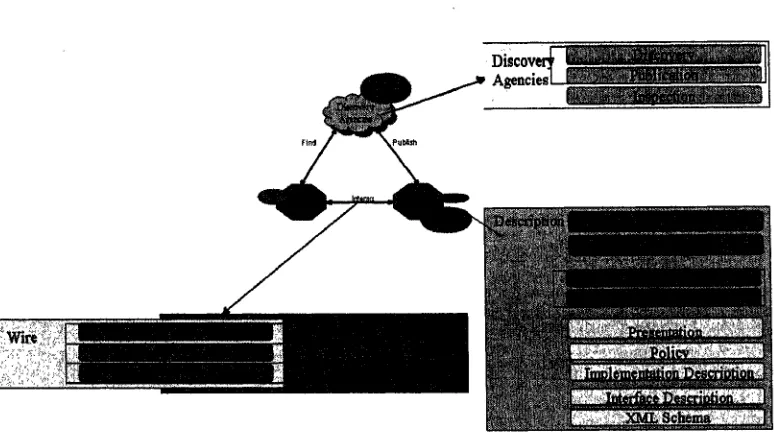
There are three key components of web service systems [Gra02]:
• wire:Comprises all technologies required to transport a service request from client to server; including XML for message encoding, and the Simple Object
Access Protocol (SOAP) for handling data transmission capabilities.
• Description:A web service interface provides a collection of operations accessible through standardized XML messaging. This interface is described using the Web
Services Description Language (WSDL), which specifies the operations provided
by a web service, including the kinds of objects that are expected as input and
the output of the operations.
• Discovery:The service requestor discovers the web service via discovery agencies
that allow service descriptions to be published and discovered. From a
performance perspective this involves the time to look up the service in the web
services directory using Universal Description Discovery and Integration (UDDI).
Figure 2.2 shows how XML messaging (SOAP), WSDL, UDDI and network
Figure 2.2 Web Service Architecture
As mentioned in section 2.2.1, the design of the interfaces is a critical
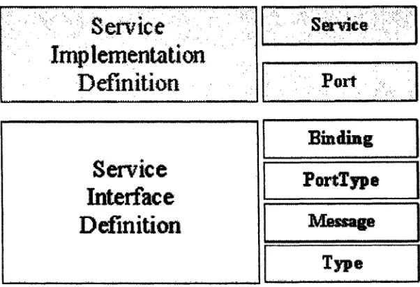
characteristic in successful design of service-oriented system. A service interface
definition is an abstract or reusable service definition that may be instantiated
and referenced by multiple service implementation definitions. In WSDL, the
service interface contains elements that comprise the reusable portion of the
service description: binding, portType, message and type elements as depicted
in Figure 2.3 - Basic Service Description below.
The service implementation definition describes how a particular service interface
is implemented by a given service provider. It also describes its location so that a
SaiH^ice
:
.Service
Implementation
Definition
Port
Service
Interface
Definition
Binding
PortType
Message
Type
Figure 2.3 Basic Service Description
Unified Modeling Language (UML) is used as a tool to describe both logical and
implementation designs, as well as specific patterns for both component and
service design. Figure 2.4 gives a Security interface in UML.
*interface»
Security
+ Logonllser ( [in] UID : String , [in] token : Token ) + GetllserName ( ) ; String
+ GetUserDomain ( ) : String
Figure 2.4: Interface in UML
2.3 Software Performance Engineering (SPE)
Software Performance Engineering (SPE) is “a method for constructing software
systems to meet performance objectives.” [Smi90] This technique proposes to
use quantitative methods and performance models in order to assess the
earliest stages of software development throughout the whole lifecycle.
Performance refers to the response time or throughput as seen by users. With
software systems becoming more complex, and handling diverse and critical
applications, the need for their thorough evaluation has become ever more
important.
Currently there are three kinds of performance evaluation techniques:
measurement, simulation and analytic modeling. Measurement technique applies
only to existing systems, so it is not suitable for performance evaluation in the
early stage of software development. While an analytic model captures the
essence of the modeled system as a set of mathematical equations, a simulation
model "mimics" the structure and behavior of the real system. The simulation
models are less constrained in their modeling power, so they can capture more
details. However, simulation models are, in general, harder to build and more
expensive to solve. In this thesis, analytic modeling is chosen due to the fact that
its cost (in terms of time and money) is lowest among the three. The Layered
Queuing Network (LQN)- the analytic model - will be used in the quantitative
performance analysis during the architectural design. LQN modeling is very
appropriate for such a use, due to fact that the model structure can be derived
systematically from the high-level architecture of the system.
2.3.1 Performance Models
Analytic models are easily solved, often interactively and provide initial feedback
on whether or not planned software is likely to meet performance goals by
producing the estimates of a set of values about the system under study with a
given set of execution conditions. These conditions may be fixed permanently in
the model, or set at runtime with free variables or parameters of the model.
Typical representations used for performance models include queuing networks
(QN), Petri nets, and a variety of proprietary simulation languages and notations.
Among them, QN model and related extensions are widely adopted by
researchers.
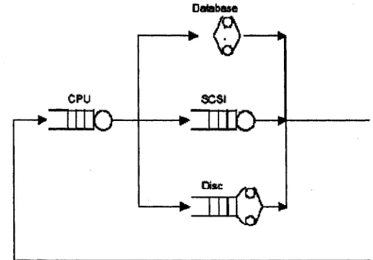
> Queuing Network Model (QN)
In 1971, Buzen proposed system modeling with Queuing Network (QN) model
and published some efficient algorithms [Buz71]. The model is constructed from
information on the computer system configuration and measurements of
resource requirements for each of the workloads modeled. The computer system
resources are represented as queues and servers. A service represents a
component of the environment that provides certain service to the software. The
queue represents jobs waiting for services and the job represents a computation
entering the system, makes requests of computer system resources. This
technique has ever since been used to represent computer system performance.
Figure 2.5 illustrates the QN model with four queues including CPU queue,
database queue, SCSI disk array and disk array
CPU SCSI
♦moo
►ztnD-J
One of the simplest QN models with some restrictions is called product-form
models. A product-form model has computationally efficient solutions such as
Mean Value Analysis (MVA). In a product-form QN model, a request is not
allowed to hold more than one resource at the same time.
> The Layered Queuing Network Model (LQN)
LQN was an extension of QN model. LQN extends the QN model to reflect
interactions between client and server processes. The processes can be shared
devices and software servers. It combines the contention of both software and
hardware component, such as processors, disks, networks. The main difference
of LQN with respect to QN is a server that receives client request and blocks
client process in the service queue. The server can also be a client to other
servers from which it requires nested services while serving its own clients. The
successive two layers form a potential sub-model of QN and the model is solved
by Mean Value Analysis (MVA) techniques. In particular, to solve the problem in
the system being modeled caused by nested calling patterns, MVA techniques
partition the input layered queuing network model into a set of smaller MVA sub
models, and then iterate among these sub models until convergence in waiting
times.
Z
a tem u// /
CM «L2//
Z—
A LQN model is represented as an acyclic graph. Nodes (also named tasks) refer
to software entities and hardware devices and arcs denote service requests.
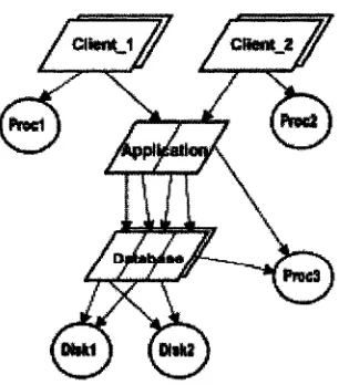
Figure 2.6 shows an example of simple LQN model for a three-tiered
client/server system. The software entities are drawn as parallelograms and the
hardware devices as circles. The nodes with outgoing and no incoming arcs play
the role of pure clients. The intermediate nodes with incoming and outgoing arcs
play both the role of client and of server and usually represent software
components. The leaf nodes are pure servers and usually represent hardware
servers (such as processors, I/O devices, communication network, etc.). Nodes
that do not receive any requests are special and they are called reference tasks
and represent load generators or users of the system.
In Figure 2.6, at the top there are two reference tasks (Client_1 and Client_2).
Each client sends requests for a specific service offered by a task named
Application, which represents the business layer of the system. Each Application
entry requires services from two different entries of the Database task, which
offers in total three kinds of services. Every task has a host processor, which
models the physical entity that carries out the operations. In Figure 2.6, P ro d ,
Proc2, Proc3, Diski and Disk2 are host processors. An arrow from an entry of
one task, say “Client_1”, to an entry of another task, say “Application”, represents
a call. A task has one or more entries that represent different operations it may
perform. A so-called entry is drawn as a parallelogram “slice”.
LQN was applied to a number of concrete industrial systems (such as database
applications, web servers, telecommunication systems, etc.) and was proven to
be useful for providing insights into performance limitations at software and
hardware levels, for suggesting performance improvements in different
> Stochastic Rendezvous Network Model (SRVN)
The Stochastic Rendezvous Network (SRVN) model [WNP+95] extends the
queuing networks to model the system with rendezvous delay. Client-server
systems with RPC calls cannot be modeled by classic queuing network model
due to the restriction to use one resource at a time.
A SRVN Model consists of the inputs tasks, entries, and phases, and the output,
throughput. Tasks represent hardware and software objects that may execute
concurrently, entries differentiate service demands at the tasks and phases
denote different intervals of service within entries. Requests for service are made
from entry to entry through send-receive-reply message interactions. Tasks do
not possess internal concurrency. The core of a SRVN model is a directed graph
whose nodes are service entries and whose arcs represent requests from one
entry to another. The SRVN model is special because it incorporates the notions
of phases and included service [FHM+95]. The execution of an entry is divided
into phases. Included service refers to the time a task is blocked waiting for a
reply after sending a request to a lower level server. However, the SRN model
has a limited capability of expression. The behavior of the system is modeled as
a task that provides service to requests in a queue. It is difficult to express the
inter task protocol.
2.3.2 Performance Analysis of Software Architecture
Software Architecture (SA) influences the achievement of quality attributes (such
as performance, security, maintainability and usability) in a software system. In
[WS02], Smith noted, “While a good architecture cannot guarantee attainment of
comments that, “quality attributes of large software systems are principally
determined by the system’s software architecture.” [KKB+98]
Architecture evaluation is considered an effective technique to address
quality-related issues early in the development lifecycle. Architectural decisions are
made very early in the software development process, therefore, it would be
helpful to be able to assess their effect on software performance as soon as
possible.
According to [AG97], software architecture represents a collection of
computational components that perform certain functions, together with a
collection of connectors that describe the interactions between components.
A number of methods, such as Architecture Tradeoff Analysis Method (ATAM)
[KBK+99], Software Architecture Analysis Method (SAAM) [KBA+94],
Architecture-Level Maintainability Analysis (ALMA) [LBB+02], and Performance
Assessment of Software Architecture (PASA) [WS02] have been developed to
evaluate quality-related issues at the software architecture level. PASA, SAAM
and ATAM are “scenario-based” where scenarios are used to provide insight into
how the architecture satisfies quality objectives. However, PASA explicitly uses
performance patterns and anti-patterns as analysis tools and for making
recommendations for improvements. The steps in the PASA method lead directly
to the construction of performance models as described in [SW02]
2.3.2.1 Performance Assessment of Software Architecture (PASA)
PASA is a method for the performance assessment of software architectures. It
uses the principles and techniques of SPE to identify potential areas of risk within
problem is found, PASA also identifies strategies for reducing or eliminating
those risks.
The PASA process consists of ten steps [WS02]:
i. Process Overview— The assessment process to familiarize both
managers and developers with the reasons for an architectural
assessment, the assessment process, and the outcomes.
ii. Architecture Overview— In this step, the development team
presents the current or planned architecture.
iii. Identification of Critical Use Cases — The externally visible
behaviors of the software that are important to responsiveness or
scalability are identified.
iv. Selection of Key Performance Scenarios— For each critical use
case, the scenarios that are important to performance are identified.
v. Identification of Performance Objectives— Precise, quantitative,
measurable performance objectives are identified for each key
scenario for each situation or performance study of interest.
vi. Architecture clarification and discussion— Participants conduct a
more detailed discussion of the architecture and the specific features
that support the key performance scenarios. Problem areas are
explored in more depth.
vii. Architectural Analysis—The architecture is analyzed to determine
whether it will support the performance objectives.
viii. Identification of Alternatives— If a problem is found, alternatives for
meeting performance objectives are identified.
ix. Presentation of Results— Results and recommendations are
x. Economic Analysis—The costs and benefits of the study and the
resulting improvements.
Among all the above steps, step vii is critical. In this step, several techniques are
brought to bear in analyzing the performance of software architecture. They
include [WS02]:
* Identification of the underlying architectural style(s)
■s Identification of performance anti-patterns
v' Performance modeling and analysis: portions of the architecture
may require more quantitative analysis. So quantitative
performance analysis is conducted and performance annotations
(such as stereotypes, tagged values defined in UML profile for SPT)
are added. The models used are deliberately simple so that
feedback on the performance characteristics of the architecture can
be obtained quickly and inexpensively.
2.3.2.2 UML Profile for Schedulability, Performance and Time (SPT)
Software Performance Engineering promotes the integration of performance
evaluation into the software development process from the early stages and
continuing throughout the whole software life cycle. Different kinds of analysis
techniques may require additional annotations to the UML model. OMG's solution
to this problem is to define standard UML profiles for different purposes. The
UML Profile for Schedulability, Performance and Time (SPT) [OMG02] adopted
for UML 1.4 defines an notations regarding schedulability and performance the
SPT Profile enables the application of the SPE methodology to systems
developed with UML for assessing the performance effects of different design
The SPT Profile contains the Performance Subprofile that identifies the main
basic abstractions used in performance analysis including stereotypes, tagged
values and constraints to represent performance requirements, the resources
used by the system and so on.
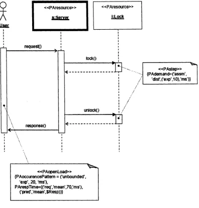
A simple example [BFW04] is given in Figure 2.7. The « P A c o n te x t» stereotype
indicates that this diagram is a scenario involving some resources (software
objects in this case) driven by a workload. The objects are a server (an active
object, indicated by the heavy box), and a lock. The annotation on the lifeline of
the user object has a « P A o p en L o a d » stereotype indicating that it is a workload,
i.e. it defines the intensity of the demand made on the system by the users of this
scenario; in this case there is an unbounded number of requests, with the interval
between requests being exponentially distributed with a mean of 20 ms. A
requirement that the mean response time is 70 ms is given, along with a
placeholder variable ($Resp) for the predicted value that will be determined by
simulation. The server offers a single operation, which requires the lock to be
acquired and released — each of these operations takes 10 ms on average.
2.3.2.3 Performance analysis with the Annotated UML model
As discussed in section 2.3.2.1, in the key step vii of PASA - Architectural
Analysis, several techniques are brought to bear in analyzing the performance of
software architecture. In the last step, performance modeling and analysis,
quantitative performance analysis based on an annotated UML model is
conducted. Three steps are involved:
• Firstly, the UML model of the software architecture is translated into a
Layered Queuing Network model (LQN) [RS95], and Stochastic
Rendezvous Network model (SRVN) [WNP95] - discussed in 2.3.1.
requests)
«P A step» {PAdemand=(‘assm’,
'disf,{‘exp’,10),'ms')} «PAresource»
l.Lock
«PAresource»
*«PAopenLoad» {PAoccurencePattem = (‘unbounded’,
‘exp', 20, ‘ms’),
PArespT«ne={freq,,’mesan,,70;ms'), (•pred7mean’,$Resp}}}
Figure 2.7 A simple sequence diagram
• In the second step, a performance analysis tool, such as the LQN solver,
conducts experiments on the performance model.
• Finally, the experiment results are fed back into the UML model to refine
The UML diagrams that provide the key information required for performance
analysis are those that describe behavior and resources:
Sequence or activity diagrams can be used to express those
scenarios that have performance requirements.
Statechart diagrams describe the behavior of active objects, and
the time required to respond to stimuli.
- Deployment diagrams define how active objects are mapped onto
processing resources.
The formalism used for building performance models in this thesis is the Layered
Queuing Network (LQN) model
The LQN model structure is generated from the high-level software architecture
that shows the high-level architectural components and their relationships, and
from deployment diagrams that indicates the allocation of software components
to hardware devices. The LQN model parameters are obtained from annotated
UML models of key performance scenarios.
The UML to LQN transformation is realized in two big steps [PZG+05]. In the first
step, the LQN model structure (i.e., the software tasks, hardware devices and
connecting arcs) is generated from the software architecture and deployment
diagrams. In the second step, the entries (which correspond to task services),
phases, activities and their parameters are derived from scenario descriptions.
Figure 2.8 [Woo02] shows an example system, representing a web-based ticket
reservation system. It uses the UML notation for the software in part (a) and the
browser
-interaet() {delay = 5 sec}
Webserver
- connect() - display() - reserveQ - confirm()
TicketDB
queryTDBQ ■ updateTDB( )
^UserNode"
Browser
« L A N »
ServerNode
W e b s e rv e r
TicketDB'
(a) UML class diagram (b) UML deployment diagram
Browser
interact
[Z = 5 s]
display
confirm
connect
reserve
UserCP
licketDB
ServerCBU
(c) Layered Queueing model
A performance analysis tool to solve the performance model has to be used in
the following step. Layered Queueing Network Solver (LQNS) is one of such
tools. LQNS combines the strengths of SRVN and MOL (Method of Layers)
solvers to broaden the modeling scope and improve the accuracy of solutions to
layered quequeing networks. The input of LQN solver is the demands at various
components such as disk, processors. The outputs of LQN solver produce are
the service time, utilizations, and throughputs of the software system.
Before the experiment results are fed back into the UML model (step three),
studying the sensitivity of performance of a system due to the effect of system
factors is very important. Sensitivity analysis (SA) can be done to study the
sensitivity of the performance (output) of a system due to the change of its
factors (input) and analyze the interaction between these factors and the effect of
each individual factor in a quantitative way. The goal of sensitivity analysis is to
3. A Statistic Approach
3.1 Problem Domain
There are growing researchers that study performance analysis. But accurate
performance analysis results need sensitivity analysis be taken into account. As
discussed in section 2.3.2.3 there are three steps in performance analysis.
Between step 2 and step 3, studying the sensitivity of performance of a system
due to the effect of system factors is very important. However, little research has
been done in service-oriented software systems and Web Service-based
systems. In [Hua04], the author did an effort. But it took into account only two
factors with one observation per treatment condition, where there is not a
clear-cut way to separate the effect of the interaction of the two factors from the
experimental error [LM74], its further discussion based on that there is no
interaction between factors. This thesis applies a statistic approach of multi
-factors in sensitivity analysis. Here -factors refer to parameters that can have an
impact on the performance of the system, such as number of users, number of
CPUs, number of threads. It provides a quantitative analysis of service-oriented
system.
3.2 Sensitivity Analysis (SA) and Design of Experiment
(DoE)
Sensitivity analysis (SA) is the study of how the variation in the output of a model
(numerical or otherwise) can be apportioned, qualitatively or quantitatively, to
different sources of variation. Its purpose is to determine how sensitive the
results of a study or systematic review are to changes in how it was done. Design
indeterminate measurements of factors and interactions between factors
statistically through observance of forced changes made methodically as directed
by mathematically systematic tables. DoE offers an empirical method of
sensitivity analysis.
Sensitivity analysis is an important aspect of performance analysis. It is very
useful for optimization of software systems and bottleneck analysis. It is common
in the early design stage that the exact values of the input parameters for the
model are unknown. Sensitivity analysis can then help in analyzing the influence
of the change in input parameters on the performance.
Design of Experiment (DOE) has been successfully used in many fields, e.g.,
physics, medicine, manufacturing. A Design of Experiment is a structured,
organized method for determining the relationship between factors (Xs) affecting
a process and the output of that process (Y). An experiment refers to a test or a
series of tests in which forced changes are made to the input variables of a
process or system on purpose so that an investigator can observe and identify
the reasons for changes that are observed in the output response.
Design of Experiments techniques provide an approach to efficiently designing
industrial experiments which will improve the understanding of the relationship
between product and process parameters and the desired performance
characteristic.
3.3 Statistic Approach
Our proposed statistic approach is a multi-factor factorial experiment. In order to
explain it more clearly, a number of terminologies and the experiment of two
In the further discussion, some terms related to experimentation are involved; the
following definitions are from [Bas96][Hic83]:
■ A hypothesis: is a tentative assumption made in order to draw out and test
its logical or empirical consequence
■ A study: is an act or operation for the purpose of discovering something
unknown or of testing a hypothesis
■ An experiment: is a study undertaken in which the investigator has control
over some conditions in which the study takes place and control over the
independent variables being studies
■ Controlled experiment: is an experiment in which the subjects are
randomly assigned to experimental conditions, the investigator
manipulates an independent variable, and the subjects in different
experimental conditions are treated similarly with regard to all variables
except the independent variable
■ Factorial treatment designs: refer to all possible combinations of the levels
of factors that are investigated in each complete trial or replication of the
experiment. It is an important type of design of experiment.
■ Factors: are defined as types of treatment such as exhaust index,
compaction method
■ Effect of a factor: is defined as the change in response caused by a
change in the level of the factor. This is also called a main effect since it
refers to the primary factors of interest in the experiment.
3.3.1
Two-factor Factorial Treatment Design
Example 3.1 is set up to demonstrate two-factor factorial treatment design
This research is to determine the effect of factors exhaust index (in seconds) and
pump heater voltage (in volts) on the pressure inside a vacuum tube (in microns
of mercury), three exhaust indexes and two voltages are chosen at fixed levels.
The levels of the factors are defined as different categories of a factor. It was
decided to run two experiments at each of these six treatment conditions (three
exhaust indexes X two voltages)
Table 3.1 shows the resulting data.
Pump Heater
Voltage
Exhaust Index
y i . .
60
90
150
127
48 28 7
189 58 | 5 3 | 33 30.5 I 15 i i |
220
62 14 9
155 54 5* 10 | 12 | 6 | 7.5
y , „ . 222 85 37 y ... =344
Table 3.1 Pressure Inside a Vacuum Tube
In table 3.1, numbers in the square are called cell mean, they are the average of
the cell.
The result can be formulized in Table 3.2:
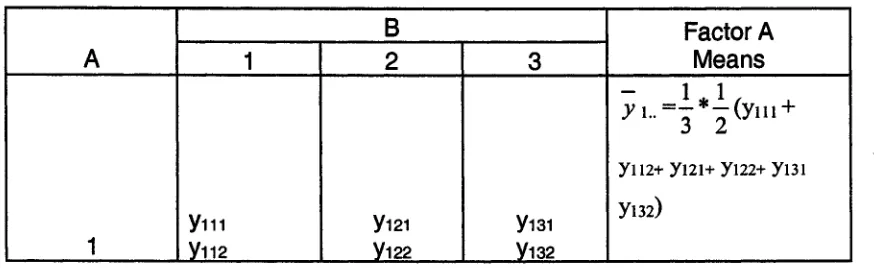
B Factor A
A 1 2 3 Means
y i.. = - * —(ym + 7 3 2
yii2+ yi2i+ yi22+ yi3i
1
ym yi2i yisi yi32)
2 y2n Y212 y22t V222 y23i V232
y 2 . . = j * ^ ( y 2 n +
y 212+ Y221+ y 222+ y 231+
ym )
Factor B Means
y -1=
1 J ,
y n 2 + y 2 ii+
y2i2>
y -2 =
yi22+ Y221+
Y222)
y ~3=
yi32+ y 231+
Y232)
_ 1 * 1 * 1 ^ y "' 2 3 2
( y m + yn2+ yi2i+ y i22+ y m yi32+ y 2 ii + y 2i2+ y 221+ y 222+ y 231 + y 232t
Table 3.2 Formulized Table Pressure Inside a Vacuum Tube
For a two-factor factorial experiment with n observations per cell, run as a
completely randomized design, a general model would be:
Yyk =
n +Ai+Bj+ABij+£ ijk
(3.1)Where A and B represent the two factors, i= 1,2,..., a level of factor A, j=1,2 b
levels of factor B, and k=1,2 n observations per cell. ^ is the population mean
which is the average of all observations, A is the effect of the /th level of the
factor A, is the effect of the /th level of the factor B, ABy is the effect of the
interaction between Ai and Bj, and e ijk is a random error component. In equation
(3.1) one tests the following hypotheses:
H0 : Aj=0 for all i
1
H0 :• Bj=0 for all j
2
Ho : ABy=0 for all i, j
3
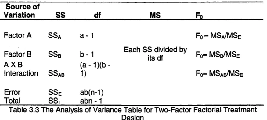
3.3.1.1 Two-factor Analysis of Variance
Let y . . denote the total observations under the ith level of factor A, y.j. denote the
total of all observations under the jth level of factor B, yy denote the total of all
observations in the ijth cell, and y... denote the grand total of all the observations.
Define y \.. ,y .j ., y y. y y . , y ... as the corresponding marginal mean for factor A,
marginal mean for factor B, cell means, and population mean. Expressed
mathematically as follows:
b n
(3.2)
7=1 k= 1
a n
/=1 k= 1
n
b
a b n
abn
i=l 7=1 k= l
The total sum of squares can be written as
(3.3)
i= l 7=1 *=1 i= l 7=1 *= i
+(
y,j. - y,.. - y.j.
+
y...
)+
(y^ - y«.
)]2
a b n a b n
+£ X X
( y tj - y i . - y . j + y - y2=1 j= 1 k=l
a b n
+ ' L ' L ' L ( y m - y t , y
2=1 j=1 &=1
^ K x , - x
..)2
+an'£(y.J..
- x - ) :
2=1 7=1
a b
+ « X X <X ~ y i - - y . j . + y - J '
2=1 7=1
a b n
X X I > i f t - > v ) 2
2=1 7=1 k= 1
Equation 3.3 can be written symbolically as
SST = SSA + SSB + SS
ab
+ SSE
Where
a b n ,, ^
2
y...
ssT
>T -
,=1 7=i *=iy*
-
n hvtS ^ - i P ' 2 - ^ b n
x , 4 2
S S B .
7
^
abn
a b v 2