CHISWELL, KAREN ELIZABETH. Model Diagnostics for the Nonlinear Mixed Effects Model with Balanced Longitudinal Data. (Under the direction of Dr. John Monahan.)
Longitudinal data, where the response for each experimental unit is measured repeatedly on several occasions, are common in biomedical (e.g., pharmacokinetic) and agricultural (e.g., growth and yield) studies. When each unit is measured at the same time points, the data are termed balanced. The methods developed in this dissertation assume balanced longitudinal data with a normally distributed response variable.
The nonlinear mixed effects model (NLMM) provides a useful statistical framework for characterizing longitudinal data when a nonlinear regression function describes the trend for each experimental unit or subject. In a simple NLMM with two stages, a nonlinear model describes the expected trajectory for each subject at the first stage. Coefficients in the first stage model are specific to each subject. At the second stage these subject-specific coefficients are modeled as random variables (random effects) from a probability distribution. Within-subject variability (e.g., due to measurement errors or fluctuations in within-Within-subject response) is modeled at the first stage. Variation between subjects is characterized by the second stage model for the random effects, some of which may be trivial (the coefficient value is the same for all subjects).
with Balanced Longitudinal Data
by
Karen Elizabeth Chiswell
A dissertation submitted to the Graduate Faculty of North Carolina State University
in partial fulfillment of the requirements for the Degree of
Doctor of Philosophy
Statistics
Raleigh, North Carolina 2007
APPROVED BY:
Dr. M. Davidian Dr. H. Zhang
Dr. H. T. Banks Dr. J. Monahan
Karen Chiswell was born in Johannesburg, South Africa, in 1972. She graduated from Roosevelt High School, Johannesburg, in 1990. In 1995 she received her Bachelor of Science in Agriculture degree, majoring in biometry, from the University of Natal (Pietermaritzburg, South Africa). After graduation, Karen worked as a forest biometrician for Mondi Forests, a forestry company with headquarters in Pietermaritzburg. In 2000, Karen moved to Raleigh, North Carolina, to pursue graduate studies in statistics at North Carolina State University. She received her Master of Statistics degree in 2002. In June of that year, Karen married Gary Faulkner.
Thank you to my adviser Dr. John Monahan for his direction, assistance, and encouragement. With him as my guide, I have learned much about statistics, research, and myself. I am grateful to my committee members, Drs. Marie Davidian, H. T. Banks, and Helen Zhang for their instruction during my graduate studies, and their attention to my research. Thank you to Drs. Woody Setzer and Hugh Barton of the Environmental Protection Agency, who drew my attention to the CCl4gas uptake experiment and the PBPK model as an interesting application.
I appreciate the wonderful opportunities provided to me as a student in the Department of Statistics at NC State University: a rich selection of course work, trusty computing resources, the chance to instruct a statistics course, and encouragement to involve myself in the life of the department. Thank you in particular to Dr. Sastry Pantula, Adrian Blue, Janice Gaddy, and Terry Byron for greasing the wheels of the department and making these things possible. I am grateful for financial support and intellectual stimulation that I gained from involvement with the Statistical and Applied Mathematical Sciences Institute (SAMSI).
List of Tables . . . xi
List of Figures . . . xvi
Nomenclature and List of Symbols . . . xxiii
1 Introduction . . . 1
1.1 Motivating Examples . . . 5
1.1.1 Carbon tetrachloride gas uptake experiment . . . 5
1.1.2 Pharmocokinetics of theophylline . . . 6
1.2 Mechanistic models . . . 8
1.2.1 Compartment models . . . 8
1.2.2 A physiologically based pharmacokinetic (PBPK) model . . . 11
1.3 Nonlinear mixed effects model (NLMM) . . . 16
1.4 First-order linearization . . . 20
1.4.1 Approximating∂f /∂β when f is the solution of a system of differential equations . . . 23
1.5 Diagnostics for the NLMM . . . 25
1.6 Literature review . . . 28
1.6.1 Model formulation and lack-of-fit of the regression function for nonlinear and mixed effects models . . . 29
1.6.2 Within-subject heteroscedasticity . . . 30
2 Exploring the marginal covariance structure . . . 36
2.1 Introduction . . . 36
2.2 Background: multivariate methods . . . 39
2.2.1 Factor analysis . . . 40
2.2.2 Principal component analysis . . . 43
2.2.3 Comparison of factor analysis and PCA . . . 48
2.2.4 Regularized or functional versions of PCA . . . 50
2.2.5 Multivariate multiple regression . . . 51
2.3 Exploring marginal covariance structure with principal component analysis . . . 54
2.3.1 Selecting the number of principal components . . . 56
2.3.2 Selection of random effects . . . 59
2.3.3 Selection of an appropriate parameterization . . . 64
2.3.4 Smoothing the PCA loadings . . . 68
2.4 Exploring marginal covariance with maximum likelihood factor analysis . . . 71
2.4.1 Maximum likelihood factor analysis whenn≤p. . . 72
2.4.2 Selecting the number of common factors . . . 75
2.4.3 Identifying and modeling within-subject heteroscedasticity . . . 78
2.4.4 Selection of random effects and an appropriate parameterization . . . 80
3 Simulation experiments: methods to explore the marginal covariance struc-ture . . . 83
3.1 Introduction . . . 83
3.2 Data generating models . . . 85
3.2.1 Example A: linear random effects . . . 86
3.2.4 Example D: Logistic model with nonlinear random effects . . . 94
3.2.5 Comparison of the nonlinear models used in examples B, C and D . . . . 97
3.3 Experiment endpoints and analysis of simulation results . . . 100
3.4 Simulation results: example A . . . 103
3.4.1 One linear random effect . . . 104
3.4.2 Two linear random effects . . . 116
3.5 Simulation results: example B . . . 127
3.5.1 One nonlinear random effect . . . 128
3.5.2 Two random effects (one linear and one nonlinear) . . . 143
3.6 Simulation results: example C . . . 156
3.6.1 One nonlinear random effect . . . 157
3.6.2 Two nonlinear random effects . . . 172
3.6.3 Two nonlinear random effects, the first one being large . . . 186
3.7 Simulation results: example D . . . 187
3.7.1 One nonlinear random effect . . . 188
3.7.2 Two nonlinear random effects . . . 204
3.7.3 Two nonlinear random effects, the first one being large . . . 216
3.8 Summary of results . . . 217
4 Detecting within-subject autocorrelation in the presence of model misspec-ification . . . 221
4.1 Introduction . . . 221
4.2 Statistical Method . . . 223
4.2.1 Multivariate regression of between-subject differences . . . 224
4.2.2 Testing for AR(1) structure in within-subject variation . . . 226
variance . . . 230
4.3.2 Experiment II: one linear random effect and heteroscedastic within-subject variance . . . 233
4.3.3 Experiment III: one nonlinear random effect and misspecification of one nonlinear parameter . . . 237
4.3.4 Summary of simulation results . . . 241
5 Application: motivating examples . . . 243
5.1 Carbon tetrachloride gas uptake experiment . . . 244
5.1.1 Exploring the marginal covariance structure . . . 246
5.1.2 Within-subject serial correlation . . . 257
5.2 Pharmocokinetics of theophylline . . . 259
5.2.1 Exploring the marginal covariance structure . . . 261
5.2.2 Within-subject serial correlation . . . 272
5.3 Summary of applications . . . 273
6 Summary and future work . . . 277
Bibliography . . . 281
Appendices . . . 286
A Functional factor analysis when k= 1 . . . 287
A.1 Functional factor model . . . 287
A.2 Penalized maximum likelihood estimation ofµ andη . . . 288
A.5 Derivation of the estimators ofµand η . . . 293
B Proofs of theorems for principal component analysis approach . . . 296
B.1 Proof of Theorem 2.3.1 (Limiting matrix of 1pYYT) . . . 296
B.2 Proof of Theorem 2.3.2 (Distribution ofg(1) when Σ=σ2Ip) . . . 298
B.3 Proof of Theorem 2.3.3 (Distribution oftr whenΣ=σ2Ip) . . . 301
C Details about maximum likelihood factor analysis . . . 304
C.1 Derivation of the MLFA objective function,Fk, when n≤p . . . 304
C.2 Minimizing the objective functionFk . . . 306
C.3 MinimizingFk whenθj <1 . . . 312
C.4 Implementing maximum likelihood factor analysis . . . 316
C.4.1 Gradient of fk with respect to diagonal elements ofΨ . . . 317
C.4.2 Computing the eigenvalues ofS∗ =Ψ−1/2SnΨ−1/2. . . 318
C.5 Behavior of the likelihood asΨdecreases orkincreases . . . 319
C.6 Maximum likelihood estimation of factor models with restrictedΨ . . . 321
C.6.1 Case 1: Ψ=σ2I p . . . 321
C.6.2 Case 2: ψj =σ2µ2jγ . . . 324
D Sensitivity equations for the PBPK model . . . 331
D.1 Sensitivity equations for body weight,Bw . . . 333
D.2 Sensitivity equations for loss rate,KL . . . 334
D.3 Sensitivity equations forVmax . . . 335
D.4 Sensitivity equations for Michaelis-Menten constant,Km . . . 336
D.5 Sensitivity equations for total cardiac output,Qc . . . 337
1.1 Typical values of CCl4 PBPK model parameters . . . 14
3.1 Simulation treatment factors for example A . . . 88
3.2 Simulation treatment factors for example B . . . 91
3.3 Simulation treatment factors for example C . . . 94
3.4 Simulation treatment factors for example D . . . 97
3.5 Properties of random effect parameters and sensitivities for the nonlinear models of examples B, C and D . . . 99
3.6 Estimated size of the PCA test for 0 common factors when there was one linear random effect . . . 105
3.7 Estimated size of the MLFA-U test for 0 common factors when there was one linear random effect . . . 107
3.8 Estimated size of the likelihood ratio tests for H0: γ = 0 when there was one linear random effect . . . 109
3.9 Estimated size of the PCA exact test when there was one linear random effect . . 111
3.10 Mean number of sensitivities included by forward selection for the experiment with one linear random effect withσ1/σ= 0 . . . 114
3.11 Proportion of cases where forward selection pickedfω(2) when σ1/σ = 0 in the experiment with one linear random effect . . . 116
3.12 Estimated size of the PCA test for 1 common factor when there were two linear random effects . . . 118
3.13 Estimated size of the MLFA-U test for 1 common factor when there were two linear random effects . . . 120
with two linear random effects whenσ2/σ= 0 . . . 125
3.16 Proportion of cases where forward selection picked fα in the experiment with two linear random effects with σ2/σ= 0 . . . 127
3.17 Estimated size of the PCA test for 0 common factors when there was one non-linear random effect in the O2C model . . . 129 3.18 Estimated size of the MLFA-U test for 0 common factors when there was one
nonlinear random effect in the O2C model . . . 131 3.19 Estimated size of the likelihood ratio tests for H0: γ = 0 when there was one
nonlinear random effect in the O2C model . . . 133 3.20 Estimated size of the PCA exact test when there was one nonlinear random effect
in the O2C model . . . 136 3.21 Mean number of sensitivities included for parameterizationf∗ by forward
selec-tion for the experiment with one nonlinear random effect in the O2C model when υδ= 0 . . . 141 3.22 Proportion of cases where forward selection picked fδ∗(2) when υδ = 0 in the
experiment with one nonlinear random effect in the O2C model . . . 142 3.23 Estimated size of the PCA test for 1 common factor when there were two random
effects in the O2C model . . . 145 3.24 Estimated size of the MLFA-U test for 1 common factor when there were two
random effects in the O2C model . . . 146 3.25 Estimated size of the likelihood ratio tests for H0: γ = 0 when there were two
nonlinear random effects in the O2C model . . . 149 3.26 Mean number of sensitivities included by forward selection when there were two
random effects in the O2C model withυω = 0 . . . 154 3.27 Proportion of cases where forward selection picked fω(2) when there were two
linear random effect in the O1C model . . . 158 3.29 Estimated size of the MLFA-U test for 0 common factors when there was one
nonlinear random effect in the O1C model . . . 159 3.30 Estimated size of the likelihood ratio tests for H0: γ = 0 when there was one
nonlinear random effect in the O1C model . . . 161 3.31 Estimated size of the PCA and MLFA-U exact tests when there was one nonlinear
random effect in the O1C model . . . 166 3.32 Mean number of sensitivities included for parameterizationf by forward selection
for the O1C model with one nonlinear random effect with υV = 0 . . . 169 3.33 Proportion of cases where forward selection pickedfV when υV = 0 in the
ex-periment with one nonlinear random effect in the O1C model . . . 172 3.34 Estimated size of the PCA test for 1 common factor when there were two random
effects in the O1C model . . . 173 3.35 Estimated size of the MLFA-U test for 1 common factor when there were two
random effects in the O1C model . . . 176 3.36 Estimated size of the likelihood ratio tests for H0: γ = 0 when there were two
nonlinear random effects in the O1C model . . . 177 3.37 Mean number of sensitivities included by forward selection when there were two
random effects in the O1C model withυC = 0 . . . 183 3.38 Proportion of cases where forward selection pickedfC when there were two
ran-dom effects in the O1C model with υC = 0 . . . 185 3.39 Estimated size of the PCA test for 0 common factors when there was one
non-linear random effect in the logistic model . . . 188 3.40 Estimated size of the MLFA-U test for 0 common factors when there was one
nonlinear random effect in the logistic model . . . 192
3.42 Estimated size of the PCA exact test when there was one nonlinear random effect in the logistic model . . . 197
3.43 Mean number of sensitivities included for parameterizationf by forward selection for the logistic model with one nonlinear random effect withυ2 = 0 . . . 200
3.44 Proportion of cases where forward selection picked fω(2) when υ2 = 0 in the experiment with one nonlinear random effect in the logistic model . . . 203
3.45 Estimated size of the PCA test for 1 common factor when there were two random effects in the logistic model . . . 204
3.46 Estimated size of the MLFA-U test for 1 common factor when there were two random effects in the logistic model . . . 206
3.47 Estimated size of the likelihood ratio tests for H0: γ = 0 when there were two nonlinear random effects in the logistic model . . . 209
3.48 Mean number of sensitivities included by forward selection when there were two random effects in the logistic model with υ1 = 0 . . . 214
3.49 Proportion of cases where forward selection picked fω(1) when there were two random effects in the logistic model with υ1 = 0 . . . 216
4.1 Simulation treatment factors for experiment I . . . 231
4.2 Estimated size of test for H0: ρ= 0 for experiment I . . . 231
4.3 Simulation treatment factors for experiment II . . . 234
4.4 Estimated size of test for H0: ρ= 0 for experiment II . . . 237
4.5 Simulation treatment factors for experiment III . . . 238
4.6 Estimated size of test for H0: ρ= 0 for experiment III . . . 238
example . . . 249 5.3 Multivariate forward selection results for the CCl4example and parameterization
f of the O2C model . . . 252 5.4 Multivariate forward selection results for the CCl4 example and the alternative
parameterization f∗ of the O2C model . . . 253 5.5 Multivariate forward selection results for the CCl4 example and the PBPK model 256
5.6 Factor analysis test results for the hypothesis thatkcommon factors are adequate for the theophylline data . . . 264 5.7 Likelihood ratio test results for structure of the specific variances in the
theo-phylline example . . . 266 5.8 Multivariate forward selection results for the theophylline example and the
volume-clearance parameterization of the O1C model . . . 270 5.9 Multivariate forward selection results for the theophylline example and the
1.1 Data from US-EPA CCl4 gas uptake experiment . . . 5
1.2 Serum concentration of theophylline following oral dose in twelve subjects. . . 7 1.3 Schematic representation of the O2C model for CCl4 gas uptake experiment . . . 8
1.4 Schematic representation of the O1C model for oral administration of theophylline 10 1.5 Schematic representation of PBPK model for CCl4 inhalation exposure in rats . 12
1.6 PBPK model predictions in chamber and liver . . . 16
3.1 Mean function and factor loadings for generating data with linear random effects in example A . . . 87 3.2 Mean and subject trajectories generated for example A with one random effect . 88 3.3 Mean and random subject trajectories described by the O2C model of example
B with random effects on ω(2) and α . . . 90 3.4 Mean and random subject trajectories described by the O1C model of example
C with random effects on Vdand Cl . . . 93 3.5 Mean and random subject trajectories described by the logistic model of example
D with random effects on ω(1) and ω(2). . . 96 3.6 Estimated power of the PCA test for 0 common factors when there was one linear
random effect . . . 105 3.7 Estimated power of the MLFA-U test for 0 common factors when there was one
linear random effect . . . 106 3.8 Estimated power of the likelihood ratio tests for H0: γ = 0 when there was one
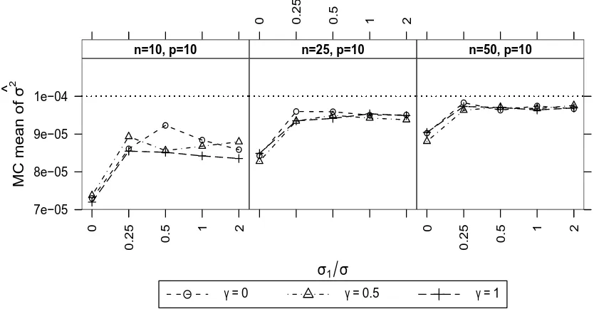
linear random effect . . . 108 3.9 Mean estimate ofσ2 from fitting the one-factor MLFA-P model when there was
there was one linear random effect . . . 113 3.12 Proportion of cases where multivariate forward selection picked the correct
sen-sitivity when there was one linear random effect . . . 115 3.13 Estimated power of the PCA test for 1 common factor when there were two linear
random effects . . . 117 3.14 Estimated power of the MLFA-U test for 1 common factor when there were two
linear random effects . . . 119 3.15 Estimated power of the likelihood ratio tests for H0: γ = 0 when there were two
linear random effects . . . 121 3.16 Mean estimate ofσ2 from fitting the two-factor MLFA-P model when there were
two linear random effects . . . 123 3.17 Mean number of sensitivities selected by multivariate forward selection when
there were two linear random effects . . . 124 3.18 Proportion of cases where multivariate forward selection picked the correct
sen-sitivities when there were two linear random effects . . . 126 3.19 Estimated power of the PCA test for 0 common factors when there was one
nonlinear random effect in the O2C model . . . 130 3.20 Estimated power of the MLFA-U test for 0 common factors when there was one
nonlinear random effect in the O2C model . . . 131 3.21 Estimated power of the likelihood ratio tests for H0: γ = 0 when there was one
nonlinear random effect in the O2C model . . . 132 3.22 Mean estimate of γ from fitting the one-factor MLFA-P model when there was
one nonlinear random effect in the O2C model . . . 134 3.23 Mean estimate ofσ2 from fitting the one-factor MLFA-P model when there was
effect in the O2C model . . . 137 3.25 Mean number of sensitivities selected by multivariate forward selection when
there was one nonlinear random effect in the O2C model . . . 140 3.26 Proportion of cases where multivariate forward selection picked sensitivities
cor-responding to a random effect on δ(2) in the O2C model . . . 143 3.27 Estimated power of the PCA test for 1 common factor when there were two
random effects in the O2C model . . . 144 3.28 Estimated power of the MLFA-U test for 1 common factor when there were two
random effects in the O2C model . . . 147 3.29 Estimated power of the likelihood ratio tests for H0: γ = 0 when there were two
random effects in the O2C model . . . 148 3.30 Mean estimate ofγ from fitting the two-factor MLFA-P model when there were
two random effects in the O2C model . . . 150 3.31 Mean estimate ofσ2 from fitting the two-factor MLFA-P model when there were
two random effects in the O2C model . . . 151 3.32 Mean number of sensitivities selected by multivariate forward selection when
there were two random effects in the O2C model . . . 153 3.33 Proportion of cases where multivariate forward selection picked the correct
sen-sitivities when there were two random effects in the O2C model . . . 155 3.34 Estimated power of the PCA test for 0 common factors when there was one
nonlinear random effect in the O1C model . . . 157 3.35 Estimated power of the MLFA-U test for 0 common factors when there was one
nonlinear random effect in the O1C model . . . 159 3.36 Estimated power of the likelihood ratio tests for H0: γ = 0 when there was one
one nonlinear random effect in the O1C model . . . 162 3.38 Mean estimate ofσ2 from fitting the one-factor MLFA-P model when there was
one nonlinear random effect in the O1C model . . . 163 3.39 Estimated power of the PCA exact test when there was one nonlinear random
effect in the O1C model . . . 165 3.40 Mean number of sensitivities selected by multivariate forward selection when
there was one nonlinear random effect in the O1C model . . . 168 3.41 Mean trace correlation for the selected multivariate regression models when there
was one nonlinear random effect in the O1C model . . . 170 3.42 Proportion of cases where multivariate forward selection picked sensitivities
cor-responding to a random effect on Vdin the O1C model with one random effect . 171 3.43 Estimated power of the PCA test for 1 common factor when there were two
random effects in the O1C model . . . 174 3.44 Estimated power of the MLFA-U test for 1 common factor when there were two
random effects in the O1C model . . . 175 3.45 Estimated power of the likelihood ratio tests for H0: γ = 0 when there were two
random effects in the O1C model . . . 178 3.46 Mean estimate ofγ from fitting the two-factor MLFA-P model when there were
two random effects in the O1C model . . . 179 3.47 Mean estimate ofσ2 from fitting the two-factor MLFA-P model when there were
two random effects in the O1C model . . . 180 3.48 Mean number of sensitivities selected by multivariate forward selection when
there were two random effects in the O1C model . . . 182 3.49 Proportion of cases where multivariate forward selection picked the correct
nonlinear random effect in the logistic model . . . 189 3.51 Estimated power of the MLFA-U test for 0 common factors when there was one
nonlinear random effect in the logistic model . . . 190 3.52 Estimated power of the likelihood ratio tests for H0: γ = 0 when there was one
nonlinear random effect in the logistic model . . . 191 3.53 Mean estimate of γ from fitting the one-factor MLFA-P model when there was
one nonlinear random effect in the logistic model . . . 194 3.54 Mean estimate ofσ2 from fitting the one-factor MLFA-P model when there was
one nonlinear random effect in the logistic model . . . 195 3.55 Estimated power of the PCA exact test when there was one nonlinear random
effect in the logistic model . . . 196 3.56 Mean number of sensitivities selected by multivariate forward selection when
there was one nonlinear random effect in the logistic model . . . 199 3.57 Mean trace correlation for the selected multivariate regression models when there
was one nonlinear random effect in the logistic model . . . 201 3.58 Proportion of cases where multivariate forward selection picked sensitivities
cor-responding to a random effect on ω(2) in the logistic model with one random
effect . . . 202 3.59 Estimated power of the PCA test for 1 common factor when there were two
random effects in the logistic model . . . 205 3.60 Estimated power of the MLFA-U test for 1 common factor when there were two
random effects in the logistic model . . . 207 3.61 Estimated power of the likelihood ratio tests for H0: γ = 0 when there were two
random effects in the logistic model . . . 208 3.62 Mean estimate ofγ from fitting the two-factor MLFA-P model when there were
two random effects in the logistic model . . . 211 3.64 Mean number of sensitivities selected by multivariate forward selection when
there were two random effects in the logistic model . . . 213 3.65 Proportion of cases where multivariate forward selection picked the correct
sen-sitivities when there were two random effects in the logistic model . . . 215
4.1 OLS PBPK model fits and residuals for the CCl4 gas uptake experiment . . . 222
4.2 Estimate ofρ for experiment I . . . 232 4.3 Estimated power to reject H0: ρ= 0 for experiment I . . . 233
4.4 Estimate ofρ for experiment II . . . 235 4.5 Estimated power to reject H0: ρ= 0 for experiment II . . . 236
4.6 Estimate ofρ for experiment III . . . 239 4.7 Estimated power to reject H0: ρ= 0 for experiment III . . . 240
5.1 Chamber concentration of CCl4 following inhalation exposure in 12 rats. . . 244
5.2 Eigenvalues ofSn for the CCl4 example. . . 246
5.3 Percentage of total sample variation variation explained by the MLFA-U and MLFA-P factor models for the CCl4 example. . . 248
5.4 Estimates of specific variancesψjbased on fitting the 2-factor MLFA-U, MLFA-P and MLFA-H models to the CCl4 data. . . 250
5.5 Estimated factor loadings for the CCl4example based on the two-factor MLFA-U
and MLFA-P models . . . 251 5.6 Sensitivities for parameters Vmax,Bw, andKL of the PBPK model . . . 257 5.7 Uncentered residuals from the multivariate regression of between-subject
differ-ences for the CCl4 example . . . 258
MLFA-P factor models for the theophylline example. . . 263 5.11 Estimates of specific variancesψjbased on fitting U, P, and
MLFA-H models to the theophylline data. . . 267 5.12 Uncentered residuals from the multivariate regression of between-subject
We use italic roman characters such asb, u and y to denote random variables, except in some cases where the context makes it clear that the realizations of these random variables are intended. Bold face italic characters such asb,uandydenote random (column) vectors, while we use bold face uppercase non-italic characters such asV orE for matrices. The subscriptT denotes the transpose of a vector or matrix. The lettert will generally indicate time. In most cases we assume that time (e.g., time when an observation is made) is not random, but fixed by design. When used in a context like f(t), letters such as f denote a known function of t. Greek characters such asβ and σ are used to denote parameters in a statistical model. When used in a context likeµ(t), Greek characters such as µdenote an unknown function oft.
The following symbols are used frequently in this dissertation with the same meaning throughout.
E - Expectation: E(y) =R ydF where F is the distribution ofy V - Variance: V(y) =E{y−E(y)}2
yij - Random variable denoting the response on thei-th subject at timetj n - Number of subjects that are observed
p - Number of observations made on a subject
yi - Random vector containing thep responses on subjecti Y - n×p data matrix with i-th row yTi
µ - Vector of means, e.g.,µ=E(yi) Σ - Covariance matrix, e.g.,Σ=V(yi) Λk - p×kmatrix of common factor loadings Ψ - p×pdiagonal matrix of specific variances
fβ - Partial derivative of functionf with respect to parameter β
Fβ - p×q matrix, the columns of which are realizations of fβ(1), . . . , fβ(q)
H0 - Null hypothesis
Introduction
In many biological studies, repeated measurements are made on a set of experimental units over time. For example, in a forestry experiment to compare the effect of spacing between adjacent seedlings on tree growth and yield, the diameters of trees in each plot are measured annually over a period of years. In an early-phase clinical trial to determine how a new drug is absorbed, distributed, metabolized and eliminated, several human subjects receive a dose of the drug. Samples of blood are drawn repeatedly from each subject over a period of hours, and the plasma concentration of the drug at each time point is measured. Such data are referred to as repeated measures data, or longitudinal data when the repeated measurements are made over time. In this dissertation we focus on longitudinal repeated measures data, but the methods developed could be applied to other types of repeated measures data where the same variable is measured repeatedly on an experimental unit or subject, and the sequence of measurements is determined by an ordered variable such as distance or length.
In the examples given above, the data are balanced by design: each experimental unit is measured the same number of times and at the same set of time points. Missing observations due, for example, to a lost blood sample, or fire damage in one corner of the forestry spacing experiment, will disrupt this balance. As the title of this dissertation implies, our methods apply to longitudinal data that are balanced. We also restrict our attention to cases where the response variable measured at each time point is a continuous variable such as concentration, blood pressure, or tree diameter, which can reasonably be assumed to follow a normal distribution.
data analysis. All methods have to take account of the correlation structure that is induced in the data because the repeated measurements made on one experimental unit are likely to be correlated with one another due to latent (unobserved) subject differences. The choice of analysis method depends to a large extent on the scientific objectives of the study. For exam-ple, in the forestry experiment, a parametric growth curve may be a reasonable model for how the diameter of an individual tree changes over time. Forestry planners would be interested in estimating the parameters of the growth curve model by fitting the model to the experiment data, and in seeing how the different spacing treatments are reflected in changes in parameter values. A nonlinear mixed effects model analysis is appropriate for this purpose. For the clinical example, a nonlinear mixed effects model analysis would also be typical.
Rice (2004) compared the functional and the more traditional longitudinal data analysis approaches (e.g,. nonlinear mixed effects models) for analyzing longitudinal data. He viewed functional data analysis as primarily an exploratory approach, whereas mixed model approaches tend to be more inferential. Sometimes the same conceptual model may be implemented in different approaches. For example, one of the structural models proposed by Jennrich and Schluchter (1986) for modeling within-subject covariance structure in a linear mixed model framework, is the factor-analytic model. Multivariate factor analysis (discussed in Chapter 2) fits this same model to describe marginal covariance structure, but does not focus on modeling the expected value of responses, as is usually the primary objective in the mixed model approach. The choice of method also depends on the structure of the data. For example, multivariate methods for repeated measures analysis require balanced data, but mixed effects approaches may be able to handle unbalanced, sparsely-sampled data, depending on the choice of covariance model.
provides estimates of typical values of the coefficients for the collected data, as well as estimates of how these coefficients vary between subjects. The estimated between-subject variation in coefficients provides important information for setting safe but effective doses for future clinical testing of the drug. In this dissertation we assume that fitting a nonlinear mixed effects model is the ultimate objective of the analysis. Section 1.3 of this chapter reviews the terminology and notation of a simple two-stage nonlinear mixed effects model.
In his 2002 Fisher Lecture titled “Variances are not always nuisance parameters,” Carroll (2003) made the point that understanding the structure of variation in data is very important. His view was that accurately modeling variance structure can be an important goal in itself (e.g., in understanding patient variability in drug response), and may have a large impact on other parts of an analysis (e.g., in predicting the working range of an assay). He included heteroscedasticity in regression (where the variance depends on known factors such as mea-surement time, or the predicted response), and the selection and modeling of random effects as two important components of variance structure. These components of variation are explicitly dealt with in the two stages of the nonlinear mixed effects model.
which coefficients should be specified as random) is valuable because state-or-the-art methods, such as those that numerically integrate out the random effects to construct a numerical ap-proximation of the marginal likelihood, are computationally expensive, or may fail, when there is an unnecessarily large number of random effects.
The methods developed in this dissertation examine three model specification issues for the nonlinear mixed effects model: selection of random effects, identification of within-subject heteroscedasticity, and identification of within-subject serial correlation. These issues and our approaches to diagnosing them are laid out in more detail in Section 1.5 of this chapter. Methods for selecting random effects and identifying within-subject heteroscedasticity are developed in Chapter 2; these methods are tested in the simulation experiments presented in Chapter 3. Chapter 4 develops a method for detecting within-subject serial correlation, in the presence of potential bias of the nonlinear regression function. In Chapter 5 we apply our methods to two real examples. Chapter 6 concludes the dissertation with a brief discussion of the limitations of our methods, which provide motivation for possible future extensions.
Time (hr)
ppm
10
15
20
0 1 2 3 4 5 6
+ + + + + + + + + + ++ + + ++++ + +++++ +++++ +++++++ o o o o o o oo oo ooo oooo oo ooo oooooo oooooooo x x x x x x x x x xx x xx xx xx xxxxx xxxxxxxx xxxxx Dose=25 ppm 30 40 50 60 70 80
0 1 2 3 4 5 6
+ + + + + + + + + ++ ++ ++ +++ ++++++ ++++++++++++ o o o o o o o o o o oo oo oo oo oooooooooo ooooooo x x x x x x x x x x x xxxx xxxx xxxx xxxxxxxxxx xxx Dose=100 ppm 100 150 200
0 1 2 3 4 5 6
+ + + + + + + + + + ++++ ++++++ ++++ ++++++++++ o o o o o o o o o o oo oo ooooo oooooooooo ooooooo x x x x x x x x x x xx xxxx xxxx xxxxxxxxxxx xxxxx Dose=250 ppm 400 500 600 700 800
0 1 2 3 4 5 6
+ + + + + + + + + + + ++ ++++ +++++++ ++++++++++++ o o o o o o o o o o oo oo ooo ooo ooooooooooo ooooo x x x x x x x x x xx xxxx xxx xxxxxxxxxxx xxxxxxx Dose=1000 ppm
Figure 1.1: Data from US-EPA CCl4 gas uptake experiment. Each panel plots data for a
dif-ferent exposure concentration. Difdif-ferent plotting symbols are used for the three animals exposed at each dose.
1.1
Motivating Examples
1.1.1 Carbon tetrachloride gas uptake experiment
Carbon tetrachloride (CCl4) is a volatile liquid that causes chemical injury to the liver through
necrosis and fat accumulation (Plaa and Charbonneau, 2000). These properties as well as the chemical’s extensive use as a grain fumigant, in the production of chlorofluorocarbons, and as a solvent in dry cleaning, makes it of interest as an air pollutant. Evans, Crank, Yang, and Simmons (1994) described a gas uptake experiment in which twelve rats were individually exposed to CCl4 in a closed chamber. Four initial exposures were used in the experiment:
1000, 250, 100 and 25 ppm. Concentration of the chemical in the chamber was measured approximately 36 times per rat over a period of 6 hours. Measurements were made at the same (or very similar) time points for all rats in the study. Figure 1.1 presents the data for the twelve rats in the gas uptake experiment.
were small differences between subjects, manifest in a clear separation of a few of the subject profiles from others. The observed profile on each subject was relatively smooth. For a given subject, we might attribute the small fluctuations around a smooth curve to measurement error or small within-subject fluctuations. We will call this latter variation,within-subject variation. The variation between trajectories will be termed between-subject variation. This might be attributed to random differences between the treatment or physiology of different subjects.
A goal of the gas uptake experiment was to predict the concentration of CCl4 over time in
the liver (these concentrations were not observed directly). This concentration can be estimated using a model that predicts the concentration of CCl4 in the liver at a given time after initial
exposure to the chemical. Mechanistic models such acompartment model or a physiologically based pharmacokinetic(PBPK) model are typically used for this type of prediction. We describe a few examples of mechanistic models in Section 1.2. Fitting the PBPK or the compartment models to the gas uptake experiment data using the nonlinear mixed model framework would allow scientists to estimate typical model coefficients characterizing the toxicokinetics of CCl4
in rats, and to quantify the expected rat-to-rat variation in these coefficients.
1.1.2 Pharmocokinetics of theophylline
Theophylline is a drug used to prevent wheezing and difficulty breathing caused by lung diseases such as asthma, emphysema, and chronic bronchitis. Davidian and Giltinan (1995, Chapter 5) described pharmacokinetic data collected from twelve human subjects given an oral dose of theophylline. On each subject, a measurement of the blood serum concentration (mg/L) of theophylline was taken before the dosing, and at ten subsequent time points over the next 24 hours. All subjects received the same dose (320 mg) of theophylline, therefore dose per unit of body weight (mg/kg) varied slightly from subject to subject. Figure 1.2 plots the measured serum concentration profiles for the twelve subjects.
As in the CCl4 example, the theophylline trajectories for different subjects showed the same
Time (hr)
Theophylline conc. (mg/L)
0 2 4 6 8 10 12
0 5 10 15 20 25
Figure 1.2: Serum concentration of theophylline following oral dose of 320 mg in twelve subjects.
concentration varied between subjects. This could be explained by variation in subject body weights, or by differences in the absorption rates of different subjects. Within-subject variation appeared to be small relative to the between-subject variation.
1.2
Mechanistic models
We use the term mechanistic model to refer to a mathematical model developed based on as-sumptions about the functional mechanics of a system. For example, most models used in pharmacokinetics are mechanistic—they make assumptions about how a drug is circulated, absorbed, metabolized, and eliminated. Mechanistic models may be simple (e.g., the open two-compartment model described in Section 1.2.1), or more complex (e.g., the PBPK model described in Section 1.2.2). Mechanistic models are typically parametric functions; their eval-uation depends on parameters which often have a physical interpretation (e.g., a metabolic rate).
1.2.1 Compartment models
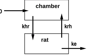
Open two-compartment model for CCl4 gas uptake experiment
A simple model for the CCl4 gas uptake data represents the exposure chamber with one
com-partment and the entire rat with a second comcom-partment. The model is represented in Figure 1.3. In this simple model, we assume that CCl4 is eliminated from the system (via metabolism,
ex-cretion, etc.) at a rate proportional to the concentration in the rat. Following from these
ke
D chamber
rat
khr krh
Figure 1.3: Schematic representation of the open two-compartment (O2C) model for for CCl4
assumptions, the system of linear differential equations
˙
zh =−khrzh+krhzr [chamber] ˙
zr=khrzh−(krh+ke)zr [rat]
(1.1)
describes this model. The initial conditions arezh(0) =Dand zr(0) = 0.
The concentration of CCl4 in the chamber at timetis given byzh(t) and the concentration in the rat is given by zr(t). The dot-notation represents a derivative with respect to time t,
˙
zh ≡ dzh(t)/dt. These quantities are model predictions, not observed data, hence our choice of the notation z instead of y; y is reserved for observed data or for random variables. Initial exposure (at time 0) in the chamber was D (dose) and we assume that initial concentration of CCl4 in the rat was 0. Transfer from the chamber to the rat due to inhalation takes place
at rate khr. The rate of transfer from rat to chamber due to exhalation is krh. The rate of elimination from the rat iske; this combines the effects of metabolism and excretion.
The differential equations (1.1) can be solved analytically for zh(t) andzr(t) and have the following closed form solution for the concentration in the exposure chamber
zh(t) =D n
β(1)exp(−β(2)t) +β(3)exp(−β(4)t)o
where D is initial exposure concentration. The coefficients β(1), . . . , β(4) are functions of the
rateskhr, krh, keand the initial exposureD. Because of the dependence of the model prediction zh(t) on β(1), . . . , β(4) we will use the notation f(t,β;D) instead of zh(t). If we assume that a dose exactly equal toDwas administered at time 0 then it is reasonable to constrainβ(1)+β(3)= 1. Under this assumption we will write the model predicting the chamber concentration of CCl4
at timet as
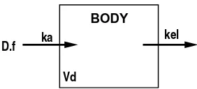
kel
BODY
ka D.f
Vd
Figure 1.4: Schematic representation of the O1C model for oral administration of theophylline. D is the administered dose, f the fraction absorbed, ka the absorption rate constant, kel the elimination rate constant, and Vd the volume of distribution.
whereα=β(1)= 1−β(3),ω(1)=β(2), andω(2) =β(4).
Open one-compartment model for oral dose of theophylline
The pharmacokinetics of theophylline in a human following oral dosing can be modeled with the open one-compartment (O1C) model with extravascular administration of drug (Ritschel and Kearns, 1998, Chapter 14). The O1C model represents the body with a single compartment and assumes a unidirectional input and output into and out of the system. This model assumes that drug entering the body distributes immediately between blood and other body tissues so that the entire body can be represented with one compartment. Figure 1.4 gives a schematic representation of the O1C model with extravascular (e.g., oral) administration of a dose D of drug. Sometimes only a fraction f of the drug may be absorbed into the body, but in the theophylline example we assume that this fraction is 100%. We assume that subjects have no previous exposure to theophylline so that theophylline concentration in the body at time zero is zero. The concentration of drug increases as absorption of drug from the gut proceeds until a peak concentration is reached. The subsequent decrease in concentration is due to elimination (excretion and metabolism) of the drug from the body.
concentration in the body, then the differential equation
˙ zb =ka
Df
Vd
exp(−kat)−kelzb (1.3)
with initial condition zb(0) = 0 describes this model (Rodda, Sampson, and Smith, 1975). The concentration of theophylline in the body at time t is given by zb(t). Absorption from the gut occurs at rate ka, andkel is the rate of elimination from the body due to metabolism and excretion.
The differential equation (1.3) can be solved analytically for zb(t) (Rodda et al., 1975) and has the following closed form solution
zb(t) = Df
Vd ka
ka−ke{exp(−kelt)−exp(−kat)}.
It is common to parameterize the elimination rate kel in terms of clearance and volume of distribution, kel =Cl/Vd. Writing the model to show explicit dependence on the parameters (ka, Cl, Vd) gives the nonlinear function
f(t, ka, Cl, Vd;D) =
Dfka Vd(ka−Cl/Vd)
exp
−Cl
Vd t
−exp(−kat)
(1.4)
for predicting the serum concentration of theophylline at time t. We assume the dose D is known (a covariate) and that f= 1.
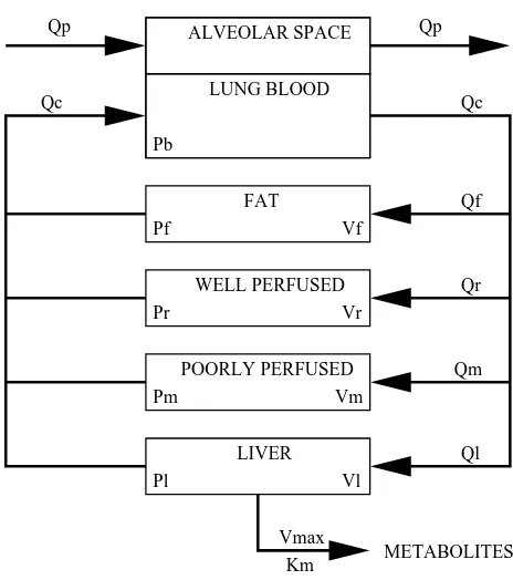
1.2.2 A physiologically based pharmacokinetic (PBPK) model
ALVEOLAR SPACE
LUNG BLOOD
FAT
WELL PERFUSED
POORLY PERFUSED
LIVER
METABOLITES
Qp Qp
Qf
Qr
Qm
Ql
Vmax Km
Vl Pl
Pm Vm
Vr Pr
Vf Pf
Pb
Qc Qc
Figure 1.5: Schematic representation of PBPK model for CCl4 inhalation exposure in rats
patterns of change in amounts or concentrations of the chemical over time in each compartment. The model is parameterized by a large number of physiological, physiochemical and bio-chemical model parameters. PBPK models are useful for prediction of target tissue (e.g., liver) concentrations, which are often not easily observed, and are believed to provide a fairly sound basis for extrapolation to different exposure routes or to different species (Evans et al., 1994).
The PBPK model that we consider here has been established as a reasonable model in rats for describing the absorption, distribution, metabolism and elimination of CCl4 and other
volatile chemicals after exposure in a closed chamber (e.g., Evans et al., 1994; Bois, Zeise, and Tozer, 1990). A schematic representation of the PBPK model is presented in Figure 1.5. This model assumes that metabolism takes place in the liver compartment via saturable enzy-matic reactions, the kinetics of which can be described by a so-called Michaelis-Menten term,
differential equations.
˙
zh =RATSQp(cx−zh/Vh)−KLzh [chamber] ˙
zf =Qf{ca−zf/(VfPf)} [fat] ˙
zr=Qr{ca−zr/(VrPr)} [rapidly perfused] ˙
zm =Qm{ca−zm/(VmPm)} [poorly perfused] ˙
zl=Ql{ca−zl/(VlPl)} −
Vmaxzl zl+KmVlPl
[liver]
(1.5)
Initial conditions at t= 0 are given by
zh(0) =zh0, zf(0) = 0, zr(0) = 0, zm(0) = 0, zl(0) = 0.
In the differential equations, the zs denote the predicted amount of CCl4 at a given time
in a particular compartment, according to the model. Subscripts indicate model compartment: subscript h is for exposure chamber, p is for pulmonary, a is for arterial, f is for fat, r is for rapidly-perfused tissue, m is for poorly-perfused tissue, and l is for liver. The function zh(t) models the expected amount of CCl4 in the chamber compartment for a particular rat.
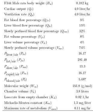
The Vs represent compartment volumes, Ps represent partition coefficients, and Qs represent blood flow or ventilation rates. The variableca is arterial concentration at timet,cv is venous concentration at timet,cx is concentration in exhaled breath at timet,KLis loss rate from the empty chamber,Vh is volume of the empty exposure chamber, and Bw is rat body weight. The parameters Vmax and Km characterize the rate of metabolism in the liver compartment. The parameterKmis the Michaelis-Menten constant, andVmaxis the maximum rate of metabolism. Table 1.1 lists typical values of the PBPK model parameters for CCl4 metabolism in
male rats. Other quantities are computed from these. A single rat was housed in each chamber in the CCl4 experiment so that RATS = 1. The initial amount in the chamber is
Table 1.1: Typical values of CCl4 PBPK model input parameters (adapted from Evans et al.,
1994)
F344 Male rats body weight (Bw) 0.182 kg
Cardiac output (Qc) 4.0 liter/hr
Ventilation rate (Qp) 4.0 liter/hr
Fat blood flow percentage (Qf c) 5% Liver blood flow percentage (Qlc) 15% Slowly perfused blood flow percentage (Qmc) 32%
Fat volume percentage (Vf c) 8%
Liver volume percentage (Vlc) 4%
Slowly perfused volume percentage (Vmc) 74%
Pliver/air (Pla) 16.17
Pfat/air (Pf a) 281.48
Pslow/air (Pma) 13.3
Prapid/air (Pra) 16.17
Pblood/air (Pb) 5.487
Molecular weight (Wm) 153.8 (g/mol)
Chamber volume (Vh) 3.8 liters
Loss rate from empty chamber (KL) 0.02 1/hr Michaelis-Menten constant (Km) 1.3 mg/liter Maximum rate of metabolism (Vmax) 0.11 mg/hr
following difference equations define relationships between other quantities in the model,
Qc=Qf+Qr+Qm+Ql, Vf +Vr+Vm+Vl= 0.91Bw cv =
1 Qc
X
∗=f,r,m,l Q∗z∗
V∗P∗, ca=
Qccv+Qpzh/Vh
Qc+Qp/Pb , cx = ca Pb.
The two metabolic parameters,Km andVmax, are usually the focus of estimation based on data from a gas uptake experiment. Other parameters in the model (such as volumes, partition coefficients, blood flow rates) may be assigned values based on other studies (e.g., partition coefficients are measured in separate in vitro studies) or from literature. This fixing of many parameters in the model at assigned values is usually done out of necessity. In most cases it is impossible to estimate all model parameters: either there are not enough observations on each subject (sometimes fewer than the number of parameters), or parameters are not well-identified. Many authors (e.g. Gelman, Bois, and Jiang, 1996) address this problem through Bayesian analysis, placing informative prior distributions on parameters. When needed, we will distinguish between those model parameters that are fixed at assigned values (we will call these parameters ξ), and those that are estimated from the data in hand (we will call these parametersβ). However, parameter estimation is not the focus of this dissertation and we will say little more about estimation.
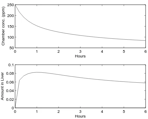
The CCl4 concentration in the exposure chamber and amount in the liver that are predicted
by the PBPK model over a six hour period are shown in Figure 1.6 for an initial exposure of 250 ppm. Model parameters were set at the values given in Table 1.1. Because of the nonlinear differential equation in the liver compartment, there is not an analytical (closed-form) solution to the system of ODEs. To evaluate the model prediction for a given set of parameter values, we computed a numerical approximation using theode45differential equation solver in Matlab (Version 7.0 (R14), The MathWorks, Inc.).
0 1 2 3 4 5 6 50
100 150 200 250
Chamber conc. (ppm)
Hours
0 1 2 3 4 5 6
0 0.02 0.04 0.06 0.08 0.1
Amount in Liver
Hours
Figure 1.6: PBPK model predictions for concentration or amount of CCl4 in chamber and
liver compartments for an initial exposure of 250 ppm. Other model parameters are given in Table 1.1.
and has an approximate closed form solution. In this case, the solution for the concentration in the chamber is a sum of 5 exponential terms. If some of the exponential rates are very small, or rates in different compartments are similar, then the predicted chamber concentration from the PBPK model looks like that from the O2C model of equation (1.2).
1.3
Nonlinear mixed effects model (NLMM)
The CCl4 gas uptake experiment data and the theophylline pharmacokinetic data described in
expected trajectory (for example with with a parametric nonlinear regression function defined by a mechanistic model), but also accounts for the correlation structure in the data by modeling between- and within-subject variability using random effects.
We will use the following notation for longitudinal data such as that collected in the two motivating examples. Suppose that n subjects are all measured p times at the same time pointst1, t2, . . . , tp. Letyij be the response (e.g., CCl4 concentration in the chamber, or serum
concentration of theophylline) measured on subjectiat time tj. It will often be convenient to write the observations made on thei-th subject as a vector of lengthp,
yi= (yi1, yi2, . . . , yip)T.
It is usual to assume that the random vectors, y1, . . . ,yn, are independent and identically distributed (i.i.d.) according to some probability distribution, for example a multivariate normal distribution. The assumption of equal time points (i.e., balanced data) is necessary for the methods developed in Chapters 2 and 4.
In Section 1.2 we described mechanistic models for modeling the expected CCl4
concentra-tion over time in the exposure chamber for a given rat, or the expected serum theophylline concentration in a particular subject. Assuming that these models adequately describe the ex-pected response for a subject, the observed trajectory might still differ slightly from the model prediction due to other sources of variation such as measurement error and within-subject fluc-tuations in metabolism rates, etc. The trajectories plotted in Figures 1.1 and 1.2 also differ between subjects. In the NLMM approach, we assume that between-subject differences are due to variation in the mechanistic model parameters over the population of subjects. The NLMM (also known as hierarchical nonlinear model) incorporates the mechanistic model, and the between- and within-subject variation into a statistical framework appropriate for describing longitudinal data.
between-subject stage) to describe longitudinal data such as those observed in the gas uptake or theophylline examples:
Stage-1: yij =f(tj,βi,ξ;xi) +εij, εij independent N(0, ψij) Stage-2: βi=β+bi, bi i.i.d. Nq(0,D)
(1.6)
forj= 1, . . . , pand i= 1, . . . , n.
In the first (subject-specific) stage of the model, yij is the observed response for subject i at measurement occasion tj, where βi is a q×1 vector of coefficients specific to subject i, ξ is a vector containing other model coefficients that are assumed known and are to be fixed at assigned values, and xi is a vector of covariates specific to subject i (such as exposure dose). The additive term εij is the subject error (due to measurement error, and other within-subject fluctuations from the mean trajectory) which is assumed to be normally distributed with variance ψij > 0. The regression function f is the nonlinear function of βi and ξ that is defined by the mechanistic model. In the case of the PBPK model where the differential equations cannot be solved analytically, the regression function f is defined implicitly, and f has to be evaluated numerically at t1, . . . , tp for given values ofβi,ξ andxi.
In the stage-1 model we have assumed the within-subject errors to be independent, but have allowed for a different variance, ψij, at each time point. It is common to assume a more parsimonious model for the variance of these errors. For example, we might assume the within-subject variance to be homoscedastic, ψij = σ2 for j = 1, . . . , p, or to assume that ψij is proportional to a power of the expected response,ψij =σ2{f(tj,βi,ξ;xi)}2γ.
The regression function f may also depend on subject-level covariates xi. In the methods developed in Chapters 2 and 4, we assume that all subjects have the same covariates, or that the data can be scaled to eliminate the effect of covariates. For example, in the models for concen-tration of CCl4 or theophylline, dividing by exposure or administered dose, D, eliminates this
the model for within-subject variation; i.e., makes variances approximately homoscedastic. In the second (between-subject) stage, we assumed that the subject-specific coefficients βi
are independent across subjects, and normally distributed with mean β and between-subject covariance matrixD. The random vectorsbiare calledrandom effects. Parameter estimation for the NLMM usually focuses on the population mean parametersβand the covariance parameters ψij and distinct elements in D. There is substantial literature on methods for estimating these parameters. Most methods are based on maximizing the marginal likelihood (based on the marginal distribution of the observed data y1, . . . ,yn) defined by the two-stage model in equation (1.6). For more details about the NLMM, its applications, and methods of estimation and inference, the interested reader is referred to a recent review by Davidian and Giltinan (2003).
One difference between the NLMM specification given in equation (1.6) and that found more commonly in the literature, is that we have parameterized the regression modelf by two types of coefficients: βi and ξ. Recall that ξ contains the coefficients that are assumed known and are not to be estimated. These assigned coefficients must, by necessity, be assumed fixed across subjects, although it is possible that they too might actually vary from subject to subject. When we need to distinguish between the true and assigned values of ξ, we will let ξ∗ denote the true value and eξ the assigned value. At some points in this dissertation where we do not concern ourselves with possible misspecification of the values ofξ (for example in Chapter 2), we have droppedξ from our notation.
1.4
First-order linearization
For now, suppose that the within-subject variances are homoscedastic, ψij =σ2 for all i and j. First-order linearization (FOL) was introduced by Beal and Sheiner (1982) as a way to approximate the marginal likelihood and compute estimates of the NLMM parameters β, σ2
and D. While the FOL approximation to the marginal likelihood may be poor, and more refined methods such as Laplace’s approximation (e.g., Wolfinger, 1993) are often favored for parameter estimation, we will make extensive use of the FOL approximation in the methods developed in this dissertation.
Let ξ∗ be the true value of the known parameters, andeξ be the assigned value. Assuming that the random effects,bi, and the differences, (ξ∗−eξ), are small, a first-order linear expansion of the true subject-specific (stage-1) regression function f(tj,β+bi,ξ∗;xi) about bi =0 and
ξ∗=eξ gives
yij ≈f(tj,β,eξ;xi) + q X
m=1
fβ(m)(tj,β,ξe;xi)·b(im)+ s X
h=1
fξ(h)(tj,β,eξ;xi)·(ξ∗(h)−ξe(h)) +εij (1.7)
wherefβ(m) =∂f /∂β(m),fξ(h) =∂f /∂ξ(h), and the partial derivatives are evaluated at (tj,β,eξ;xi).
The partial derivatives are also referred to as sensitivity functions or parameter sensitivities. In Section 1.4.1 we discuss approximation of the sensitivities when f is evaluated numerically by solving a system of differential equations.
Let f(i)= [f(t1,β,eξ;xi), . . . , f(tp,β,eξ;xi)]T,F(βi) be a p×q matrix with (j, m)-th element fβ(m)(tj,β,eξ;xi), andF(ξi) be ap×smatrix with (j, h)-th elementfξ(h)(tj,β,eξ;xi). Then (1.7) can be written in vector notation as
yi ≈f(i)+F(βi)bi+F(ξi)(ξ∗−eξ) +εi. (1.8)
equa-tion (1.6) with ψij ≡ σ2, we can see that the marginal distribution of yi is approximately normal, with marginal mean and covariance given approximately by the following expressions:
E(yi) =E[E(yi|bi)]≈E[f(i)+F(βi)bi+Fξ(i)(ξ∗−eξ)] =f(i)+Fξ(i)(ξ∗−eξ)≡µi,
and
Cov(yi) = E[V(yi|bi)] +V[E(yi|bi)]
≈ E[V(εi)] +V[f(i)+F(i) β bi+F
(i)
ξ (ξ∗−eξ)] = σ2Ip+Fβ(i)D F(βi)T
≡ Σi.
The mean vector µ(i) and the covariance matrix Σi depend on the parameter values β and eξ (this dependence is suppressed in the notation). In this dissertation, since our focus is not on estimatingβ or ξ, approximate values will be substituted. For example, for the PBPK model we could use values in Table 1.1.
The dependence of these expressions on iis through the covariate vectorxi. If all subjects have the same covariate values, xi ≡x (e.g., they all have the same initial dose D), then the vectorsyi, i= 1, . . . , nwill be independent and approximately identically distributed according to the multivariate normal distribution with approximate marginal mean vector
µ=f +Fξ(ξ∗−eξ)
and approximate marginal covariance matrix
In this case, an approximate model for yi is
yi ≈µ+Fβbi+εi. (1.10)
If the random effects, bi, or the misspecification errors, ξ∗−eξ, are not small, then the FOL approximation of equation 1.10 will be poor. In Chapter 2, we assume that an approximation that is linear in the random effects bi is adequate. However, if some random effects are large, then second-order terms may need to be added to the Taylor series approximation of equa-tion (1.7). This will involve second order partial derivatives of f, and quadratic functions of the random effects in bi.
One of the model diagnostic objectives to be discussed in Section 1.5 is to discriminate between two parameterizations of a model based on the structure of the marginal covariance. The FOL approximation is also the basis of this diagnostic. Letf∗(t,δ
i,ξ;x) be an alternative parameterization off with subject-specific coefficientsδi =δ+di. Assuming that the random effects di and the misspecification errors (ξ∗−eξ) are small, the first-order linear expansion of the alternative stage-1 regression functionf∗(t
j,δ+di,ξ∗;xi) about di=0 and ξ∗ =eξ gives
yij ≈f∗(tj,δ,eξ;xi) + q∗ X
r=1
fδ∗(r)(tj,δ,ξe;xi)·d(ir)+ s X
h=1
fξ∗(h)(tj,δ,eξ;xi)·(ξ(∗h)−ξe(h)) +εij
wheref∗
δ(r) =∂f∗/∂δ(r) evaluated at (tj,δ,eξ;xi). Assuming constant covariates and, we arrive
at the approximate model foryi based on the parameterization f∗,
yi ≈µ∗+F∗δdi+εi. (1.11)
whereµ∗ and F∗δ are defined for the alternative parameterizationf∗ in the same manner that
µand Fβ were defined for parameterizationf.
value of β such that f∗(t
j,δ,eξ;xi) = f(tj,β,eξ;xi). At this value of β it will also be the case that f∗
ξ(h)(tj,δ,eξ;xi) = fξ(h)(tj,β,eξ;xi). Thus µ= µ∗ and comparing the approximations in equations (1.10) and (1.11), we see that the difference between parameterizationsf and f∗ will potentially be manifest (to first-order) by the terms involving the random effects and sensitivity functions,Fβbi and F∗δdi. We develop this idea further in Section 2.3.3 of Chapter 2.
1.4.1 Approximating∂f /∂β when f is the solution of a system of differential
equations
The partial derivative∂f /∂βof a parametric model functionf(t, β) with respect to a parameter βis known as aparameter sensitivity. The sensitivity is a function of the variablet, and depends on the value of the parameterβ∗ where it is evaluated. The sensitivity reflects how rapidly the functionf changes for small changes inβ when β is near β∗.
The sensitivities are often used to reflect the degree of dependence of model predictions on particular parameter values. Since the true parameter values in a model are seldom known, knowing how sensitive a model’s predictions are to small changes in parameter values provides useful information about the degree of uncertainty due to misspecification of a particular param-eter value. The sensitivities are also used in other ways. For example in statistical applications such as nonlinear regression, the large sample estimate of the covariance matrix of the param-eter estimates can be computed from the partial derivatives of the function with respect to the parameters. Numerical optimization methods will often make use of the partial derivatives of the objective function with respect to its arguments; these partial derivatives are typically functions of the parameter sensitivities.
to a system of ordinary differential equations (ODEs). In this case the sensitivities must be approximated numerically. Suppose thatβis a single model parameter under consideration and letf(t, β)≡z(t, β) be the required model prediction obtained by solving a differential equation inz. The partial derivative off with respect toβ could be computed using a finite difference approximation, for example a central difference
[z(t, β+h)−z(t, β−h)]/(2h).
An alternative approach when z is defined by a system of differential equations is to solve a new system of differential equations called the sensitivity equations. The latter approach (also know as internal differentiation or variational equations) is preferable to the finite difference approximation: the computational costs being similar to the costs of finite differencing, but the accuracy being higher, especially when low accuracy methods are used to approximate z (e.g., Ostermann, 2004; Dalgaard and Larsen, 1990).
In order to explain the derivation of the sensitivity equations, suppose that the solution z(t, β) depends on a single parameterβ and is defined by a single differential equation
˙
z(t, β) =F(z(t, β), β)
with initial conditionz(t0, β) =z0(β). Recall that the dot-notation denotes differentiation with
respect to time, ˙z = dz/dt. Taking partial derivatives with respect to β on both sides of the differential equation gives
∂
∂βz(t, β) =˙ ∂
∂zF(z, β)· ∂
∂βz(t, β) + ∂
∂βF(z, β)
by the Chain Rule for derivatives. Letz[β](t, β) =∂z(t, β)/∂β denote the partial derivative of
z(t, β) with respect toβ. This is the sensitivity function that we seek. Assuming that we may
of zand z[β] on (t, β), we can re-write this last equation as
˙
z[β]= ∂
∂zF(z, β)·z[β]+ ∂
∂βF(z, β). (1.12)
This is a differential equation for the required sensitivity function z[β]. The initial condition for this equation is obtained by differentiating the original initial condition with respect toβ, giving
z[β](t0, β) =
∂ ∂βz0(β).
The differential equation for z[β] is a function of z, and must be solved simultaneously with
the original differential equation for z. In Appendix D we derive the sensitivity equations for several parameters of the PBPK model.
1.5
Diagnostics for the NLMM
In this dissertation we assume that a preliminary fit of the has been made, and that estimates of the coefficients in the nonlinear function are in hand. We view the methods developed in the following chapters as providing a set of diagnostic tools for assessing certain assumptions of the NLMM. Our methods provide guidance for formulating a realistic but parsimonious version of the NLMM to be fitted after the preliminary analysis. The methods developed in this dissertation examine three model specification questions for the nonlinear mixed effects model.
it is likely that some of the parameter values will be more similar across subjects than others. Our goal is to identify the subset of parameters that require non-trivial random effects.
Our approach to identifying the non-trivial random effects is based on the FOL approxima-tion,
yi ≈µ+Fβbi+εi for i= 1, . . . , n.
This approximation is similar to a multivariate common factor model,
yi =µ+Λkui+εi
that explains the structure of the marginal covariance withklinear random effects called com-mon factors. By fitting the comcom-mon factor model to the data and looking at the relationship between the p×k loadings matrix Λk and the p×q sensitivity matrix Fβ we identify which elements inβ require non-trivial random effects. This approach is developed in Chapter 2.
The question of random effects selection can also be looked at from the viewpoint of identify-ing a parameterization of the nonlinear function that characterizes the between-subject variation with a few random effects. As pointed out in Section 1.4, under a different parameterization f∗ of the nonlinear regression function, the FOL approximation for the data becomes
yi ≈µ+F∗δdi+εi.
By examining the relationship between Λk and F∗δ, and comparing results with those for the original parameterizationf, we may be able to pick one parameterization that provides a simpler explanation of between-subject variation than another.
comparing the fits of factor models with different assumptions about ψj, we can detect the presence of within-subject heteroscedasticity, and possibly also propose an appropriate model for within-subject variation. For example, comparing two factor models, the first withψj =σ2 (homoscedasticity) and a second with ψj =σ2µ2jγ (power-of-the-mean), we can judge whether the power-of-the-mean model provides a better description of within-subject variation than the homoscedastic model.
The factor model and the simple NLMM of equation (1.6) assume that the within-subject residuals εij in the stage-1 model are independent within subject. Examining whether this is a reasonable assumption, or whether there is evidence of within-subject serial correlation, is the third issue addressed in this dissertation. Exploring this question is complicated by potential bias in the nonlinear regression function. Even if the mechanistic model is true, it could be difficult to estimate all the coefficients from one data set, especially if there are many parameters, as in the PBPK model for the CCl4 example. Some coefficients might be assigned
known values that are erroneous, eξ6=ξ∗, leading to model misspecification and bias,
E(yij|tj,β
i,ξ∗;x) =f(tj,βi,ξ∗;x)6=f(tj,βi,eξ;x).
Model bias makes it difficult to tease out the presence of time-dependence in the within-subject residuals. A method for detecting within-subject correlation in the presence of misspecified co-efficient values is developed in Chapter 4. Our approach is based on the FOL of equation (1.8). For subjectsiand i′ with the same covariate values, the between-subject difference is approxi-mately
yi−yi′ ≈Fβ(bi−bi′) + (εi−εi′)
and the effect of misspecification ofξ cancels out, at least approximately. Diagnosis of within-subject serial correlation is then based on the residuals after regressing vectors of differences,