DOI: 10.1534/genetics.103.021055
Conditional Probability Methods for Haplotyping in Pedigrees
Guimin Gao,* Ina Hoeschele,*
,1Peter Sorensen
†and Fengxing Du
‡*Virginia Bioinformatics Institute and Department of Statistics, Virginia Tech, Blacksburg, Virginia 24061,†Department of Animal Breeding
and Genetics, Danish Institute of Agricultural Sciences, 8830 Tjele, Denmark and‡The Monsanto Company, Chesterfield, Missouri 63198 Manuscript received August 6, 2003
Accepted for publication April 29, 2004
ABSTRACT
Efficient haplotyping in pedigrees is important for the fine mapping of quantitative trait locus (QTL) or complex disease genes. To reconstruct haplotypes efficiently for a large pedigree with a large number of linked loci, two algorithms based on conditional probabilities and likelihood computations are presented. The first algorithm (the conditional probability method) produces a single, approximately optimal haplo-type configuration, with computing time increasing linearly in the number of linked loci and the pedigree size. The other algorithm (the conditional enumeration method) identifies a set of haplotype configura-tions with high probabilities conditional on the observed genotype data for a pedigree. Its computing time increases less than exponentially with the size of a subset of the set of person-loci with unordered genotypes and linearly with its complement. The size of the subset is controlled by a threshold parameter. The set of identified haplotype configurations can be used to estimate the identity-by-descent (IBD) matrix at a map position for a pedigree. The algorithms have been tested on published and simulated data sets. The new haplotyping methods are much faster and provide more information than several existing stochastic and rule-based methods. The accuracies of the new methods are equivalent to or better than those of these existing methods.
H
APLOTYPING in a pedigree refers to the recon- Green1987;SobelandLange1996;Sobelet al.1996; struction of haplotypes from observed genotype LinandSpeed1997;Thomaset al. 2000;Abecasiset al. data within the pedigree. It is an important computa- 2002). The rule-based procedures are deterministic and tional step in the fine mapping of quantitative trait locus fast and hence can be used for large pedigrees with or complex disease genes in animal and human com- large numbers of linked loci, but they do not use the plex pedigrees. For a simple, small pedigree with a small distance between markers and are not suitable for situa-number of linked loci, it is not difficult to enumerate all tions with substantial amounts of missing data or unin-possible consistent haplotype configurations, calculate their formative markers. The likelihood- or conditional prob-likelihood or conditional probabilities, and identify the ability-based algorithms are typically stochastic (Sobel most probable configurations (Sobelet al.1996). A con- andLange1996;Sobelet al.1996;LinandSpeed1997; sistent haplotype configuration is an assignment of hap- Thomaset al. 2000), and although they can be applied to lotypes to all individuals in the pedigree, which is consis- complex pedigrees, their computing time requirements tent with all observed genotype data and the pedigree may become unacceptable.structure. However, for larger and more complex pedi- In the space of all consistent haplotype configurations grees and with a larger number of linked loci, the num- on a pedigree (SACHC), typically most configurations ber of consistent haplotype configurations is usually too have very small probabilities conditional on the observed large for an exhaustive search to be feasible. Methods genotype data, so that only a relatively small subset of that are capable of handling a larger number of loci are configurations is relevant. In this contribution, we pro-not guaranteed to find the most probable configuration vide two new methods, a conditional probability
approx-(LinandSpeed1997). imation and a conditional enumeration method. The
Various computer algorithms and programs for hap- first method produces a single, approximately optimal lotyping in pedigrees have been developed. Some of these haplotype configuration. The second method eliminates algorithms are purely logical and rule based (Wijsman haplotype configurations with low conditional
probabil-1987;O’Connell2000;Tapadaret al2000;Qianand ities from SACHC, identifies a subset of haplotype
con-Beckmann2002), while others are based on likelihood
figurations with high conditional probabilities, ranks the or conditional probability computations (Landerand
configurations in the subset by their likelihood, and cal-culates their numbers of recombinants. These methods use the closest informative flanking markers, which may 1Corresponding author:Virginia Bioinformatics Institute, 1880 Pratt
not be the immediate flanking markers of a locus under Dr., Bldg. XV (0477), Virginia Tech, Blacksburg, VA 24061-0477.
E-mail: [email protected] consideration, and information from close relatives,
ents, and offspring. For a large pedigree with a large optimal haplotype configuration from SACHC, by as-signing a haplotype pair to each individual in the pedi-number of linked loci, both new methods are not
guar-anteed to find the most probable configuration and gree sequentially in a given order, on the basis of the conditional probabilities. This method is designed for the true configuration. Below we first describe our new
methods and subsequently compare them with Sim- pedigrees of small or moderate size and a small number of linked loci. We use a similar, sequential approach to Walk2 (SobelandLange1996;Sobelet al.1996) and
the methods of Lin and Speed (1997) andQian and reconstruct a haplotype configuration for the person-markers inU, and we extend it to larger pedigrees and
Beckmann(2002).
larger numbers of loci by an approximation method. We assign an ordered genotype to each unordered METHODS person-marker in Usequentially in a given order {M1,
M2, . . . ,Mt}. We note that this is different from assigning
Notation and definitions: In this article, we assume
an optimal haplotype pair to each individual. The order that all individuals in a pedigree have been genotyped
in which the assignment occurs is termed a reconstruc-for all markers. The combination of a specific individual
tion order. After the first i ⫺ 1 person-markers have and a specific marker locus is termed a person-marker,
been assigned the set of ordered genotypesm1,m2, . . . , and each person-marker either is homozygous or has
mi⫺1, the two ordered genotypes at person-markerMiare
an observed heterozygous genotype with two possible
compared by means of their conditional probabilities ordered genotypes. A multilocus genotype of an
individ-Pr(mi|m1, . . . , mi⫺1,D). The miwith the higher
condi-ual with an ordered genotype at each locus is termed
tional probability is assigned to person-markerMi.
Con-a hCon-aplotype pCon-air. For eCon-ach founder in the pedigree, we
catenating these conditionally optimal ordered geno-look for the first heterozygous locus in the linkage group
types provides an approximately optimal haplotype and assign arbitrarily an ordered genotype for this locus.
configuration for thetperson-markers inUand hence For some descendants in the pedigree, the genotypes
for the entire pedigree. at some heterozygous loci can be ordered with certainty
Consequently, at each step of the algorithm, the con-conditional on parental genotypes (Pong-Wong et al.
ditional probabilities of the ordered genotypes at a per-2001; Qian and Beckmann 2002), so that haplotypes
son-marker, Pr(mi|m1, . . . ,mi⫺1,D), must be calculated. can be partially reconstructed with certainty. Our
haplo-Exact calculation will be time consuming and is there-type reconstruction methods are based on this prior,
fore approximated. The conditional probability method partial reconstruction (PPR). The observed data in a
with the approximation is termed the conditional proba-pedigree after PPR are denoted byD.
bility approximation. The approximation is described A person-marker with an observed, unordered,
het-next. erozygous genotype is referred to as an unordered
per-Assume a given reconstruction order {M1, M2, . . . , son-marker. For a pedigree with Nmembers and a set
Mt}, letMirepresent the person-marker for locusjand
ofLlinked marker loci, there arekiunordered
person-individual k, and assume that the first i ⫺ 1 person-markers (U1
i, . . . ,Ukii) in individualiafter PPR, where
markers have been assigned the ordered genotypesm1,
Uj
i denotes the jth unordered person-marker in
in-m2, . . . , mi⫺1. Also, let Vjk denote the subset of loci,
dividuali. The set of all unordered person-markers in
which contains locusjand all loci with known ordered a pedigree is denoted by U ⫽ {U1
1, . . . , U
k1 1, . . . ,
genotypes in individual k after the assignment of
or-U1
N, . . . ,U kN
N}. To reconstruct the haplotype
configura-dered genotypes to the firsti⫺1 person-markers. Then tion for the entire pedigree, one needs to reconstruct only
conditional probabilities at person-markerMi, Pr(mi|m1, the haplotype configuration for the person-markers inU.
. . . ,mi⫺1,D), can be calculated approximately by condi-Let t⫽兺N
i⫽1ki denote the total number of unordered
tioning only on marker information at loci inVj kfrom
person-markers in the pedigree, let {M1, M2, . . . , Mt}
individual kand those of its “close” relatives, parents, be a specific ordering of the person-markers inU, and
and offspring, which have a known, ordered genotype letmi⫽ai1/ai2denote an ordered genotype for
person-at locusj, or marker Mi, where allele ai1 is of paternal origin. The
joint probability of a haplotype configuration for the Pr(mi|m1, . . . ,mi⫺1,D)⬇Pr(mi|Gk,Gf,Gm,Hoff), (2) person-markers in U, {m1,m2, . . . ,mt}, conditional on
whereGk,Gf, andGmare the partially ordered multilocus the pedigree data after PPR (D), can be factored using
genotypes at the loci inVj
kof individualk, its father and
the method of decomposition for a given order, or
its mother, respectively, and Hoff is the set of partially Pr(m1,m2, . . . ,mt|D)⫽Pr(m1|D)Pr(m2|m1,D) known haplotypes, inherited from individual k, by all of its offspring, all after PPR and assignment of {m1,m2, . . . , . . . Pr(mt|m1, . . . ,mt⫺1,D).(1)
mi⫺1} to person-markers {M1,M2, . . . ,Mi⫺1}. If any of the relatives of individual khas an unordered genotype at Conditional probability approximation: Sobel et al.
from Equation 2. If all close relatives of individual k
have unordered genotypes at locusj, then Pr(mi|m1, . . . ,
mi⫺1,D)⫽0.5. A partially ordered multilocus genotype of an individual has a known (fixed) ordered genotype at some loci (the genotype list of this individual contains only one element for these loci), while it has two possible ordered genotypes at some other loci (the genotype list contains two elements for these loci). A partially known haplotype has known parental origin at some loci (the allele list of this haplotype contains only one allele for these loci), while it has unknown parental origin at some other loci (the allele list contains two alleles for these loci).
At the loci inVj
k,Gkhas only one unordered
person-markerMi(at locusj), and the two ordered genotypes
at person-marker Mi are denoted by m1i and m2i. Let
G1
k(G2k) be the corresponding multilocus genotypes
ob-tained fromGkwith ordered genotypem1i (m2i) at locus
j. Then
Pr(m1
i|Gk,Gf,Gm,Hoff)⫽Pr(G1k|Gk,Gf,Gm,Hoff)
⫽ Pr(G1k|Gf,Gm)Pr(Hoff|G1k)
兺
2n⫽1Pr(Gnk|Gf,Gm)Pr(Hoff|Gnk)
.
(3)
A marker is informative for an individual and one of its parents, if the ordered genotype is known for both relatives, and if the parent is heterozygous. After the assignment of {m1,m2, . . . ,mi⫺1} to person-markers {M1,
Figure1.—Pedigree with eight individuals and seven
mark-M2, . . . , Mi⫺1}, for the person-markerMiin individual
ers: (*) the person-marker (individual 4, locus 3), whose
or-k, letMf
LandMfRdenote the closest informative flanking dered genotype probabilities are to be computed; (.,.) an markers for individual kand its father; let Mm
L and MmR unordered genotype (the other genotypes are ordered). For be defined analogously for individualkand its mother; the ordered genotypes, the left allele is of paternal origin. The information in boxes is not used to calculate the conditional and letMo
Land MoR be defined similarly for individual
probabilities of the ordered genotypes at locus 3 in individual
k and its offspring o. Let Gn
k(MoL,Mi,MoR) denote the
4. Individuals 1, 2, 3, and 5 are not founders, but rather their subset of ordered genotypes at lociMo
L,Mi, andMoR in ancestry is omitted, as it is not needed here. the multilocus genotypeGn
k of individual k(n⫽ 1, 2);
letfHnk(MfL,Mi,MfR) andmHnk(MmL,Mi,MmR) be the pater-nal and materpater-nal haplotypes at loci Mf
L, Mi, and MfR If either of the two closest informative flanking mark-and atMm
L,Mi, andMmR, respectively, in the multilocus ers for one of the close relatives and individualkdoes genotypeGn
kof individualk; letHooff(MLo,Mi,MoR) be the not exist, then this flanking marker is dropped from haplotype containing only lociMo
L,MiandMoRinherited the corresponding transmission probability in Equation by offspring o from individual k; let Gf(MLf,Mi,MfR) 4; if there are no informative flanking markers for a andGm(MmL,Mi,MmR) denote the ordered genotypes at close relative and individual k, then this relative is loci Mf
L, Mi, and MfR and at MmL, Mi, and MmR in the dropped from Equation 4; and if there are no informa-multilocus genotypes Gf of the father and Gm of the tive flanking markers for any of the close relatives and mother, respectively. From Equation 3 we have
individualk, then Pr(m1
i|Gk,Gf,Gm,Hoff)⫽
Pr*(fH1
k|Gf)Pr*(mH1k|Gm)兿oPr*(Hooff|G1k) 兺2
n⫽1Pr*(fHnk|Gf)Pr*(mHnk|Gm)兿oPr*(Hooff|Gnk) Pr(m1
i|Gk,Gf,Gm,Hoff)⫽ 0.5. (4)
To illustrate the approximation method, we use a where
three-generation pedigree with partially ordered geno-Pr*(fHn
k|Gf)⫽Pr(fHkn(MfL,Mi,MfR)|Gf(MLf,Mi,MfR)),
types at seven markers in eight individuals as depicted Pr*(mHn
k|Gm)⫽Pr(mHkn(MmL,Mi,MmR)|Gm(MmL,Mi,MRm)),
and explained in Figure 1. Pr*(Ho
off|Gnk)⫽Pr(Hoffo (MoL,Mi,MoR)|Gnk(MoL,Mi,MoR)), n⫽1, 2.
We consider calculating the conditional probabilities of the ordered genotypes at locus 3 in individual 4. For For example, Pr(fHnk(MfL,Mi,MRf)|Gf(MfL,Mi,MfR)) is the
this calculation, only the marker information of the transmission probability of haplotypefHnk(MLf,Mi,MfR) by
used, whereV3
4⫽[1, 2, 3, 5, 7]. The genotype data in boxes are discarded temporarily for calculating the con-ditional genotype probabilities at this person-marker (locus 3, individual 4), but may of course be used for other person-markers (e.g., locus 5 in individual 6). Marker information at loci 4 and 6 are not used, because individual 4 is not ordered at these loci, and the marker data of individual 8 are not used because this offspring has an unordered genotype at locus 3. In individuals 6 and 7, only the haplotypes inherited from individual 4 are used. At locus 5 of individual 6, for example, the genotype is not ordered, and hence the paternal haplo-type of individual 6 inHoff contains two alleles (1 and 2) in the allele list for this locus. For locus 3 in individual 4, the closest informative flanking markers are markers 1 and 5 for individual 4 and its father, markers 2 and 5 for individual 4 and its mother, and markers 2 and 7 for individual 4 and offspring 6.
A problem with the conditional probability approxi-mation method is that the reconstruction order can greatly influence the conditional probability of the re-constructed haplotype configuration. Therefore, it is
Figure2.—Simulated pedigree data for illustration of in-important to determine an approximately optimal
re-fluence of reconstruction order on the haplotype reconstruc-construction order and to execute the conditional
proba-tion result. The distance between adjacent markers is 1 cM. bility method with this order. Because we identify an (*) The person-markers requiring reconstruction; (.,.) an un-ordered genotype for each person-marker inUon the ordered genotype (the other genotypes are ordered). For the
ordered genotypes, the left allele is of paternal origin. basis of the information from the individual under
con-sideration and its close relatives, we assign ordered geno-types earlier to those person-markers that have more
in-with eight markers in six individuals, which is depicted formation in the individual and its close relatives than
in Figure 2. The distance between two adjacent markers to others. Thus, the conditional probability method is
is 1 cM. We treat the ordered genotype at four person-implemented with the following steps:
markers as unknown (marked with * in Figure 2). So 1. Calculate the probabilities of the ordered genotypes
the set of all unordered person-markers in this pedigree for each person-marker inUconditional on the data
is U⫽ {U1
2,U14,U15,U61}, which denotes the set of un-D, retain the larger probability for each person-marker,
ordered person-markers in individuals 2, 4, 5, and 6 at and determine the person-marker with the highest
locus 8.
probability. This person-marker is set toM1. Then Table 1 shows the process to determine an approxi-the ordered genotype with higher probability,m1, is mately optimal reconstruction order (M
1,M2,M3,M4), assigned toM1. which is not unique, and the corresponding reconstruc-2. Calculate the probabilities of the ordered genotypes
tion result with the conditional probability approxima-for all remaining person-markers in the subset ofU,
tion. Table 2 lists the reconstruction results for another U⫺{M1}, conditional onm1andD, retain the larger arbitrarily chosen reconstruction order (U1
2,U14,U15,U16) probability for each person-marker, and determine
for comparison. The ordered genotypes assigned to the person-marker inU⫺{M1} with the highest prob- person-markerU1
2differ between the two orders, so the ability. This person-marker becomesM2, and the or- corresponding haplotype configurations for the person-dered genotypem2, having the larger probability of markers inUare different. The configuration with the the two choices, is assigned toM2. approximately optimal order has a higher conditional 3. Similarly, order and assignment for the remaining
probability, Pr(U1
4 ⫽1/2, U15⫽2/1, U16 ⫽ 1/2, U12⫽ person-markers are determined, resulting in an
ap-2/1|D)⫽(0.98)3· 0.998⫽0.9393, than the configuration proximately optimal orderM1, . . . ,Mtand a
corre-obtained with the other order, Pr(U1
2⫽1/2,U14⫽1/2, sponding assignmentm1,m2, . . . ,mt.
U1
5⫽2/1,U16⫽1/2|D)⫽0.961 · (0.667)3 ⫽0.2852. Conditional enumeration method:In an approximately To illustrate how to reconstruct haplotypes for a
pedi-optimal reconstruction orderM1,M2, . . . ,Mt, the
condi-gree with the conditional probability approximation in
tional probability approximation method sequentially an approximately optimal order and to show the
influ-identifies an approximately optimal ordered genotypemi
ence of reconstruction order on the result, we simulated
or-TABLE 1
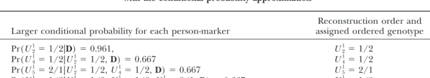
Haplotype reconstruction in an approximately optimal order (M1,M2,M3,M4)
with the conditional probability approximation
Optimal reconstruction order and assigned Larger conditional probability for each person-marker ordered genotype
Pr(U12⫽1/2|D)⫽0.961, Pr(U14⫽1/2|D)⫽0.980,
Pr(U15⫽2/1|D)⫽0.980, Pr(U16⫽1/2|D)⫽0.980; M1⫽U14⫽1/2 Pr(U1
2⫽1/2|U14⫽1/2,D)⫽0.5, Pr(U1
5⫽2/1|U14⫽1/2,D)⫽0.980, Pr(U1
6⫽1/2|U14⫽1/2,D)⫽0.980; M2⫽U15⫽2/1 Pr(U1
2⫽2/1|U14⫽1/2,U15⫽2/1,D)⫽0.961, Pr(U16⫽1/2|U
1
4⫽1/2,U 1
5⫽2/1,D)⫽0.980; M3⫽U 1 6⫽1/2 Pr(U12⫽2/1|U
1
4⫽1/2,U 1
5⫽2/1,U 1
6⫽1/2,D)⫽0.998 M4⫽U 1 2⫽2/1
dered genotype and the corresponding haplotype config- of the two probabilities for two possible ordered ge-notypes at M conditional on the data (D) and m1. urations from SACHC, until all configurations but one
(approximately optimal) configuration have been elimi- Find the person-marker with the highest conditional probability pl
2 among the t ⫺ 1 remaining person-nated. This elimination process causes some loss of
infor-mation. It is therefore preferable to retain a subset of markers inU⫺{M1}. Denote this person-marker byM2 and its two possible ordered genotypes byms
2 andml2 configurations with high conditional probabilities over a
single configuration. This was achieved by modification whose conditional probabilities satisfy Pr(ms
2|m1,D)ⱕ Pr(ml
2|m1,D). For each of the ordered genotypesm1 of the conditional probability approximation method,
re-sulting in the conditional enumeration method, which retained for person-markerM1, if Pr(ml2|m1,D)ⱖ , then assign thisml
2to person-markerM2and eliminate consists of the following steps:
the other ordered genotype. Otherwise, if Pr(ml 2|m1, 1. For any person-markerMinU, letpl
1denote the larger D)⬍ , retain both ordered genotypes for person-one of the two probabilities for the two possible
or-markerM2. dered genotypes atM conditional on the data (D).
3. Similarly, for each combination of retained ordered Find the person-marker with the highest conditional
genotypesm1,m2, . . . ,mi⫺1for the firsti⫺1 person-probabilitypl
1among thetperson-markers inU.
De-markers, find the person-markerMiand retain one
note this person-marker by M1 and its two possible
or both ordered genotypes for person-markerMi, on
ordered genotypes by ms
1andml1whose conditional
the basis of Pr(m2
i|m1,m2, . . . ,mi⫺1,D) and. probabilities satisfy Pr(ms
1|D) ⱕ Pr(ml1|D). Let
be a threshold (0.5 ⱕ ⱕ 1), e.g., ⫽ 0.96. If After all unordered person-markers have been pro-cessed with this algorithm, a set of haplotype configura-Pr(ml
1|D)ⱖ , then assign thisml1to person-marker
M1and eliminate the other ordered genotype. Other- tions has been retained. This set is denoted by SACHC*. The configurations in SACHC* can be ranked by their wise, if Pr(ml
1|D)⬍ , retain both ordered genotypes
for person-markerM1. likelihood, and a smaller subset of configurations with high likelihood from SACHC* can be obtained by elimi-2. For each ordered genotype m1(m1can bems1orml1)
assigned to M1, and for any person-marker M in nating other configurations, as desired.
The accuracy of the enumeration method and the the set of t ⫺ 1 remaining person-markers in U,
denoted by U⫺ {M1}, let pl2 denote the larger one number of configurations in SACHC* increase with
in-TABLE 2
Haplotype reconstruction in an arbitrary order, different from that in Table 1, with the conditional probability approximation
Reconstruction order and Larger conditional probability for each person-marker assigned ordered genotype
Pr(U12⫽1/2|D)⫽0.961, U12⫽1/2 Pr(U14⫽1/2|U
1
2⫽1/2,D)⫽0.667 U
1 4⫽1/2 Pr(U15⫽2/1|U
1
2⫽1/2,U 1
4⫽1/2,D)⫽0.667 U
creasing value. When ⫽ 1, this method becomes the exhaustive enumeration method (Sobelet al.1996), and SACHC⫽ SACHC*. The exhaustive enumeration method is exact, but it becomes computationally expen-sive or infeasible for large pedigrees with large numbers of loci. When ⫽ 0.5, the conditional enumeration method becomes the conditional probability approxi-mation method, which is always fast computationally, but it provides only a single approximately optimal hap-lotype configuration. The SACHC* identified by the conditional enumeration method (0.5⬍ ⬍1) always contains the single, approximately optimal haplotype configuration identified by the conditional probability method ( ⫽ 0.5). The SACHC may contain a subset of haplotype configurations all having the same and highest conditional probability. The conditional proba-bility method cannot identify this subset, but the condi-tional enumeration method can identify all or most of the configurations in this subset. The number of haplo-type configurations retained in SACHC*, the accuracy, and the computing time for the conditional enumera-tion method can be controlled with the value of(see below).
RESULTS FOR A PUBLISHED DATA SET
To compare our methods with existing methods, we
analyzed a published data set, which was previously ana- Figure3.—The most likely haplotype configuration for the Krabbe disease pedigree (nine individuals, eight marker loci). lyzed bySobelet al.(1996) andLinandSpeed(1997).
The left allele at any locus in any individual is of paternal The data came from a medical genetic study of the
origin. Krabbe disease byOehlmannet al. (1993) in a pedigree
of nine individuals with unordered genotypes at eight
polymorphic markers on chromosome 14, with marker Using the conditional enumeration method with ⫽ order D14S47, D14S52, D14S43, D14S53, D14S55, 0.995, SACHC* contained 128 haplotype configurations, D14S48, D14S45, and D14S51, and with distances be- which were selected from the 32,768 configurations in tween adjacent markers of 12.5, 22.3, 3.3, 8.4, 1.9, 18.8, SACHC. The computation time wasⵑ2 sec, much less and 1.5 cM. than that of the exhaustive enumeration method ( ⫽ The approximately optimal haplotype configuration 1). The total conditional probability of the 128 configu-identified with the conditional probability approxima- rations in SACHC* accounted for 99.89% of the total tion ( ⫽0.5) is shown in Figure 3 and is identical to probability of all the configurations in SACHC, and the the most likely configuration obtained by Sobel et al. SACHC* contained all of the 50 top configurations in
(1996) andLinandSpeed(1997). The computing time SACHC, except for the two configurations ranked 36 of the conditional probability approximation was ⬍1 and 39 (with conditional probabilities of 0.00034 and sec on 2.00 GHz Intel Xeo n CPU (1,047,546 kB RAM; 0.00029, respectively). The 10 configurations with the Microsoft Windows 2000). highest like-lihoods and conditional probabilities in After PPR, SACHC had a total of 32,768 configura- SACHC* were the same as the 10 top configurations in tions. Using the exhaustive enumeration method ( ⫽ SACHC listed in Table 3.
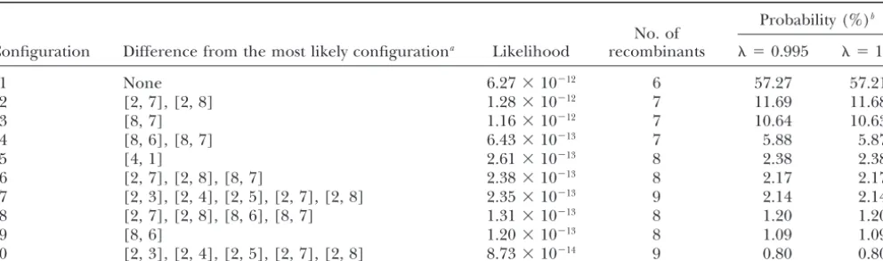
TABLE 3
Haplotype configurations with highest likelihoods identified by the conditional enumeration method and numbered from 1 to 10 by decreasing likelihood or conditional probability
Probability (%)b
No. of
Configuration Difference from the most likely configurationa Likelihood recombinants ⫽0.995 ⫽1.0
1 None 6.27⫻10⫺12 6 57.27 57.21
2 [2, 7], [2, 8] 1.28⫻10⫺12 7 11.69 11.68
3 [8, 7] 1.16⫻10⫺12 7 10.64 10.63
4 [8, 6], [8, 7] 6.43⫻10⫺13 7 5.88 5.87
5 [4, 1] 2.61⫻10⫺13 8 2.38 2.38
6 [2, 7], [2, 8], [8, 7] 2.38⫻10⫺13 8 2.17 2.17
7 [2, 3], [2, 4], [2, 5], [2, 7], [2, 8] 2.35⫻10⫺13 9 2.14 2.14 8 [2, 7], [2, 8], [8, 6], [8, 7] 1.31⫻10⫺13 8 1.20 1.20
9 [8, 6] 1.20⫻10⫺13 8 1.09 1.09
10 [2, 3], [2, 4], [2, 5], [2, 7], [2, 8] 8.73⫻10⫺14 9 0.80 0.80
aFor example, [2, 7] denotes that the corresponding configuration has an ordered genotype at marker 7 of individual 2,
which differs from that in the most likely configuration.
bThe conditional probability estimated by the ratio of the likelihood to the sum of the likelihoods of all configurations in
SACHC*. When ⫽1.0, the conditional probabilities are calculated exactly.
tions in SACHC*. When ⫽1, the conditional probabil- with those of SIMWALK 2 (Sobel and Lange 1996;
Sobel et al. 1996), we simulated several pedigrees as ities are calculated exactly.
described below. Using their Gibbs-Jump method,LinandSpeed(1997)
Data simulation:Founder haplotypes were generated identified their most and second-most likely
configura-assuming Hardy-Weinberg equilibrium within and link-tions with estimated conditional probabilities of 0.69
age equilibrium between loci. Haplotypes for nonfound-and 0.15, respectively. These two configurations are
ers were then simulated conditional on their parental identical to configuration 1 (with highest likelihood)
haplotypes, assuming Haldane’s no interference map-and configuration 3 (with third-highest likelihood) in
ping function. Table 3, respectively. The conditional probabilities
esti-The first pedigree had 88 members (20 founders) mated by Lin and Speed (1997) are higher than the
over five generations. The linkage group consisted of corresponding values in Table 3, and configuration 2,
20 biallelic markers with allele frequency of 0.5 and with which has a higher likelihood than configuration 3,
a distance between adjacent markers of 1 cM. Each was missed. The Gibbs-Jump method was executed to
parent had one spouse, and each full-sib family had two identify the configurations and probabilities in a very
children. The likelihood of the simulated haplotype short run time of⬍1 min on a Sun SPARC 20
worksta-configuration was 1.3329 ⫻ 10⫺81and the number of tion for 100 cycles of the Gibbs and Metropolis jumping
recombinants was 18. steps, which likely caused the failure to identify
configu-Several additional pedigrees with SNP and microsatel-ration 2 and the overestimation of the conditional
prob-lite markers were simulated similarly. The first four pedi-abilities (LinandSpeed1997).
grees had 330 members (30 founders) with SNP markers Application of the rule-based minimum-recombinant
over six generations. The linkage group consisted of 10 haplotyping method of Qian and Beckmann (2002)
biallelic markers. Each parent had two spouses, and would identify only configuration 1, which has the
mini-each full-sib family had three children. The four pedi-mum number of recombinants. Moreover, several
con-grees differed in the allele frequency (0.5 or 0.9) and figurations in Table 3 have eight recombinants, but
dif-in the distance between adjacent markers (0.5, 1, and ferent likelihoods, and recombinant counting cannot
3 cM). The fifth (sixth) pedigree had 546 members and discriminate among these configurations. The
optimal-42 founders over seven generations with SNP markers ity criteria based on likelihood and recombinant count
(microsatellite markers having 10 alleles each) and the are equivalent, or produce the same ranking of the
con-same structure as the 330-member pedigrees, but in-figurations, only if the distances among adjacent
mark-termarker distance was 1 cM, frequency for each allele ers are all equal and if all markers are informative.
was 0.5 (0.1), and the linkage group consisted of 40 markers.
Results for simulated pedigrees:Table 4 presents the SIMULATION STUDIES
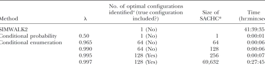
TABLE 4
Comparison of the haplotype reconstruction results of the new methods and SIMWALK2 from the analysis of the 88-member pedigree
No. of optimal configurations
identifieda(true configuration Size of Time
Method included?) SACHC* (hr:min:sec)
SIMWALK2 1 (No) 41:39:35
Conditional probability 0.50 1 (No) 1 0:00:01
Conditional enumeration 0.965 64 (No) 64 0:00:06
0.990 64 (No) 128 0:00:06
0.995 128 (Yes) 256 0:00:07
0.997 128 (Yes) 69,632 0:27:45
aEach of the (approximately) optimal configuration(s) identified by any of the methods had the same
likelihood as the true configuration. This likelihood is the estimated (approximately) highest likelihood over all configurations in SACHC. The true highest likelihood is unknown (exhaustive search not feasible).
figurations had the same likelihood as the true (simu- configuration had a higher likelihood and a lower num-ber of recombinants than the true configuration. As lated) configuration. This likelihood is the estimated
(ap-proximately) highest likelihood over all configurations noted earlier, any SACHC* identified with the condi-tional enumeration method contains the single, approx-in SACHC. The true highest likelihood is unknown
(ex-haustive search not feasible). imately optimal haplotype configuration identified with the conditional probability method.
SIMWALK2 had to be restarted several (three) times
before it identified a (single) approximately optimal For each pedigree, Table 5 presents results for several (ascending) values. In particular, column 7 contains configuration, whose likelihood had the same value as
the likelihood of the true configuration. The likelihoods the ratio of the sums of the likelihoods of all configu-rations in two different SACHC* corresponding to two of the configurations obtained prior to the final run
were much lower, and the corresponding recombinant differentvalues (current row over previous row). For example, for the first 330-member pedigree (inter-counts were higher. The two new methods identified
configurations with the same likelihood as the true con- marker distance 0.5 cM), 1.045 is the ratio of the total likelihood for the SACHC* corresponding to ⫽0.995 figuration in just one run and were much faster than
SIMWALK2. For 0.965 ⱕ ⱕ 0.997, the conditional to the total likelihood for the SACHC* corresponding to ⫽0.965. The results in column 7 indicate that when enumeration method identified a subset of 64–128
hap-lotype configurations with likelihood and recombinant thevalue and the size of SACHC* become sufficiently large, an additional increase inoften results in a very counts equal to those of the true configuration. To
identify such a subset with SIMWALK2, the required large increase in the size of SACHC* but only a very small increase in the total likelihood. For example, for multiple starts and restarts would probably take several
weeks, instead of seconds and minutes with the condi- the second 330-member pedigree (intermarker distance 1 cM, allele frequency 0.5), when was raised from tional enumeration method. For ⬎0.995, the number
of configurations with the estimated highest likelihood 0.990 to 0.995, the size of SACHC* increased 319 times, but the total likelihood increased only by 4.2%. For equal to that of the true configuration did not increase,
but the number of configurations in SACHC* and the the fourth 330-member pedigree (intermarker distance 3 cM, allele frequency 0.5), the increase in the total computing time increased rapidly.
Results of the conditional enumeration method for likelihood, due to increasingand the size of SACHC*, was higher when compared with the increases for the the four 330-member pedigrees and the 546-member
pedigrees are presented in Table 5. For each of the six pedigrees with shorter intermarker distances (1 and 0.5 cM).
pedigrees, the conditional probability approximation
identified an approximately optimal haplotype config- The results in Table 5, column 8, show that a few hundred up to 1000 of the top configurations (those uration with approximately highest likelihood in ⬍1
sec. When the distance between adjacent markers was with the highest likelihoods) always contained most of the information in SACHC*. The exception was the 1 or 0.5 cM, the haplotype configuration identified by
the conditional probability approximation had likeli- pedigree with the largest intermarker distance of 3 cM. In this case, determining SACHC* with a largervalue hood equal to or higher than that of the true
TABLE 5
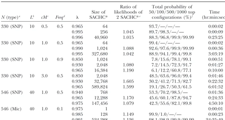
Reconstruction results of the conditional enumeration method for the 330-member pedigrees and the 546-member pedigrees with different marker allele frequencies
and distances between adjacent markers
Ratio of Total probability of
Size of likelihoods of 50/100/500/1000 top Time
N(type)a Lb cMc Freqd SACHC* 2 SACHC*e configurations (%)f (hr:min:sec)
330 (SNP) 10 0.5 0.5 0.965 64 93.7/—/—/— 0:00:02 0.995 256 1.045 89.7/98.3/—/— 0:00:09 0.996 40,960 1.015 88.3/96.8/99.9/99.99 0:23:25 330 (SNP) 10 1.0 0.5 0.965 64 99.4/—/—/— 0:00:02 0.990 1,024 1.088 92.6/97.6/99.9/99.99 0:00:36 0.995 327,680 1.042 88.9/94.1/99.4/99.8 3:03:19 330 (SNP) 10 1.0 0.9 0.850 1,024 7.8/15.6/78.1/99.1 0:00:51 0.930 2,048 1.080 7.2/14.5/72.3/91.7 0:01:27 0.965 16,384 1.190 6.1/12.2/60.8/77.1 0:10:00 330 (SNP) 10 3.0 0.5 0.850 2,048 48.5/63.6/96.0/99.4 0:01:46 0.930 32,768 1.605 30.2/41.2/71.3/82.7 0:22:32 0.965 589,824 1.599 19.1/26.7/50.3/61.5 6:01:52 546 (SNP) 40 1.0 0.5 0.940 768 53.3/70.2/98.5/— 0:01:36 0.965 12,288 1.170 45.6/60.1/87.8/94.7 0:24:33 0.975 147,456 1.079 42.3/55.6/82.1/89.8 4:50:10
546 (Mic) 40 1.0 0.1 0.975 1 0:00:01
0.985 128 1.149 99.9/1.0/—/— 0:00:23 0.991 524,288 1.126 98.1/98.9/99.9/99.99 24:35:49
aNdenotes the number of individuals in the pedigree, and type denotes the marker type, where SNP (Mic)
denotes SNP (microsatellite) markers.
bNumber of linked marker loci. cDistance between adjacent markers.
dAllele frequency. For the microsatellite markers, each allele has the frequency 0.1.
eThe ratio of the sums of the likelihoods of all configurations in two different SACHC* corresponding to
two differentvalues (current row over previous row).
fSum of likelihoods of top configurations over sum of likelihoods of all configurations in SACHC*; top
configurations are those with highest likelihood in SACHC*.
tances (ⱕ1 cM), retaining at most a few hundred up to Finally, Table 5 also shows that when marker allele frequency increased from 0.5 to 0.9 (330-member pedi-1000 of the top configurations in SACHC* for further
inference, such as the calculation of an identity-by-de- grees), the increase in the number of homozygous geno-types resulted in a decrease of the information content scent (IBD) matrix in fine mapping of quantitative trait
loci (QTL), should often preserve most of the informa- of the markers and an increase in the computing time of the conditional enumeration method (for the same tion while significantly reducing computing time.
Ex-pectedly, the size of SACHC* and the computing time values). increased considerably with increasing intermarker
dis-tance (for the samevalues).
DISCUSSION When the number of alleles at each locus increases
from 2 to 10 (546-member pedigrees in Table 5), the We have presented a conditional probability approxi-mation and a conditional enumeration method for hap-information in the pedigree increases because of the
increase in the number of informative genotypes. Con- lotyping in pedigrees. The conditional probability ap-proximation method identifies a single, approximately sequently, the computing time of the conditional
enu-meration method decreases for the samevalue, and optimal (in terms of likelihood or conditional probabil-ity) haplotype configuration in a very short run time. For the identified sets of top configurations account for
higher conditional probabilities (Table 5, column 8). any given threshold ⬎0.5, the conditional enumeration method finds a set of configurations (SACHC*), which For the 546-member pedigree with 10 alleles at each
locus, the total conditional probability of the 50 top always contains a subset of configurations with approxi-mately highest likelihood. In the set SACHC*, some configurations is almost equal to 1. When ⫽0.991,
the conditional probability of the top configuration configurations may have very low likelihood, and some configurations with relatively high likelihood may not (0.773) is⬎50 times the conditional probability of the
configurations from SACHC* can be obtained by elimi- unordered person-markers inUafter PPR, hence with the number of linked loci and the size of the pedigree. nating the configurations with low likelihood as desired.
The second problem can be controlled through the The computing time of the conditional enumeration method is controlled by the value ofand increases at choice of the value for, subject to computational
feasi-bility, as for ⫽1 no configuration will be missed. In most exponentially with the size of a subset of unordered person-markers inUand linearly with its complement. our experience with simulated data (as presented in
this article and beyond), when the distance between The subset includes every person-marker, where the prob-abilities of both ordered genotypes are less thanduring adjacent markers is⬍1.5 cM, then it is possible to set
to high values (e.g., ⱖ0.96) while maintaining com- the reconstruction process (seeConditional enumeration
method). Computing time of the haplotype
reconstruc-putational efficiency. However, when the distance
ex-ceeds 2 cM, settingto high values may cause a substan- tion for the same value ofis influenced by the inter-marker distance and the pedigree structure: it decreases tial increase in computing time.
Both methods sequentially assign ordered genotypes with increasing relationship/inbreeding coefficients, in-creasing size of the full-sib and half-sib families, and to the unordered person-markers in a pedigree in
ap-proximately optimal orders, by using only the marker decreasing number of founders.
A subset of marker haplotype configurations with information of the individual under consideration and
its close relatives (parents and offspring), and condi- high likelihoods identified by the conditional enumera-tion method can be used to calculate the IBD matrix tional on previously assigned ordered genotypes of other
person-markers preceding the current one in the order for a pedigree at a specific genome location (for defini-tion of IBD matrix, see Pong-Wong et al. 2001). The chosen.
In the rule-based method of Qian and Beckmann IBD matrix conditional on the observed data (D) is a weighted average of all IBD matrices, each conditional (2002), the haplotype assignment is based on
minimiz-ing the number of recombinants by considerminimiz-ing two on a haplotype configuration in SACHC, where the weight of each configuration is the conditional probabil-generations at a time, a nuclear family or a
parent-off-spring trio. In contrast, our methods are based on max- ity of the configuration in SACHC. The IBD matrix conditional on the observed data (D) can be calculated imizing the probability of the ordered genotype at each
unordered person-marker conditional on the marker in- by the expression formation of close relatives in three generations.
More-QD⫽
兺
i
QiPr(i|D) (5)
over, when the intermarker distances are not equal, or when markers are not fully informative, then some
(Wang et al. 1995; Hoeschele 2001), where i is a
haplotype configurations with the same recombinant
specific haplotype configuration of the pedigree in count may have different likelihoods, and the rankings
SACHC, andQD(Qi) is the IBD matrix of the pedigree
based on likelihood and recombinant count may not
be identical (e.g., in Table 3, configurations 5, 6, 8, and givenD(i). Pr(i|D) is the probability oficonditional
on the observed dataD. The summation in Equation 5 9 have the same number of recombinants but different
is over all configurations in SACHC. For a large pedigree likelihoods; configuration 7 has one more recombinant
with a large number of loci, the IBD matrixQDcan be
but a higher likelihood than configurations 8 and 9).
estimated approximately by Equation 5 with the summa-The accuracy of the conditional enumeration method
tion over the subset of configurations identified by the can be increased by raising the value ofand retaining
conditional enumeration method, and the probability a larger fraction of the top configurations in SACHC*,
Pr(i|D) can be estimated approximately by the ratio
which in turn increases computing time for the
haplo-of the likelihood haplo-ofito the sum of the likelihoods of
type reconstruction and, more importantly, for
subse-all configurations in the identified subset. quent inferences. While accuracy of haplotype
reconstruc-In this article we demonstrated applications of the tion is somewhat difficult to define when the pedigree
new methods to pedigrees with up to 546 members and is too large to perform an exhaustive search, we
evalu-40 linked loci. We anticipate that pedigrees of several ated it for two differentvalues by the ratio of the sums
thousand individuals and up to 100 linked loci can be of the likelihoods of all configurations in two different
analyzed efficiently by choice of suitablevalues without SACHC* corresponding to the twovalues and by the
significant loss in accuracy of evaluation of the IBD fraction of the total conditional probability in SACHC*
matrix and QTL localization (work in progress). explained by the retained subset of configurations with
In this contribution, we have assumed that all individ-highest likelihoods. Accuracy comparisons based on
sub-uals in a pedigree have been genotyped for all markers. sequent inference (such as the accuracy of QTL fine
We have work in progress on extending our methods mapping with IBD matrices calculated from different
to pedigrees with missing marker data (the haplotypying subsets of retained haplotype configurations) remain to
methods presented in this article were implemented in be performed (work in progress).
a C⫹⫹program, which is available upon request from The computing time of the conditional probability
mosome 14 by multipoint linkage analysis. Am. J. Hum. Genet. We thank Keying Ye and Nan Bing for helpful comments and
sug-53:1250–1255. gestions. This research was supported by grant R01 GM66103-01 from
Pong-Wong, R., A. W. George, J. A. WoolliamsandC. S. Haley, the National Institutes of Health and a grant from the Monsanto
2001 A simple and rapid method for calculating identity-Company to I. Hoeschele.
by-descent matrices using multiple markers. Genet. Sel. Evol.33:
453–471.
Qian, D., andL. Beckmann, 2002 Minimum-recombinant haplotyp-ing in pedigrees. Am. J. Hum. Genet.70:1434–1445.
LITERATURE CITED Sobel, E., andK. Lange, 1996 Descent graphs in pedigree analysis: applications to haplotyping, location scores, and marker sharing
Abecasis, G. R, S. S. Cherny, W. O. CooksonandL. R. Cardon, statistics. Am. J. Hum. Genet.58:1323–1337.
2002 Merlin-rapid analysis of dense genetic maps using sparse Sobel, E., K. Lange, J. R. O’ConnellandD. E. Weeks, 1996 Haplo-gene flow trees. Nat. Genet.30:97–101. typing algorithms, pp 89–110 inIMA Volumes in Mathematics and
Hoeschele, I., 2001 Mapping quantitative trait loci in outbred pedi- Its Applications,Vol. 81: Genetic Mapping and DNA Sequencing, edited grees, pp. 599–644 in theHandbook of Statistical Genetics, edited by T.Speedand M. S.Waterman. Springer-Verlag, New York. by D. J.Balding, M.Bishopand C.Cannings. John Wiley & Sons, Tapadar, P., S. GhoshandP. P. Majumder, 2000 Haplotyping in Chichester, UK. pedigrees via a genetic algorithm. Hum. Hered.50:43–56.
Lander, E. S., andP. Green, 1987 Construction of multilocus ge- Thomas, A., A. Gutin, V. AbkevichandA. Bansal, 2000 Multilocus netic linkage maps in humans. Proc. Natl. Acad. Sci. USA84: linkage analysis by blocked Gibbs sampling. Stat. Comput.10:
2363–2367. 259–269.
Lin, S., andT. P. Speed, 1997 An algorithm for haplotype analysis. Wang, T., R. L. Fernando, S. van der BeekandJ. A. M. van Aren-J. Comput. Biol.4:535–546. donk, 1995 Covariance between relatives for a marked
quantita-O’Connell, J. R., 2000 Zero-recombinant haplotyping: applications tive trait locus. Genet. Sel. Evol.27:251–274.
to fine mapping using SNPs. Genet. Epidemiol.19 (Suppl 1): Wijsman, E., 1987 A deductive method of haplotype analysis in S64–S70. pedigrees. Am. J. Hum. Genet.41:356–373.
Oehlmann,R., J.Zlotogora, D. A.Wengerand R. G.Knowlton,