R E S E A R C H
Open Access
Numerical solution of nonlinear fuzzy
Fredholm integral equations of the second
kind using hybrid of block-pulse functions
and Taylor series
Mahdy Baghmisheh
1and Reza Ezzati
2**Correspondence: [email protected] 2Department of Mathematics, Karaj Branch, Islamic Azad University, Karaj, Iran
Full list of author information is available at the end of the article
Abstract
The main purpose of this paper is to introduce a method of successive
approximations in terms of a hybrid of Taylor series and a block-pulse function, which is given for solving nonlinear fuzzy Fredholm integral equations of the second kind and the error estimate of the approximation solution. Finally, two numerical examples are presented to show the accuracy of the proposed method.
Keywords: nonlinear fuzzy Fredholm integral equation; hybrid of block-pulse function and Taylor series
1 Introduction
The study of fuzzy integral equations (FIE) from both theoretical and numerical points of view has been developed in recent years after a distinct study of the existence of a unique solution for fuzzy Fredholm integral equations had been carried out in []. The Banach fixed point theorem is the main tool in studying the existence and uniqueness of the so-lution for fuzzy integral equations which can be found in [–]. Numerical procedures for solving fuzzy integral equations of the second kind, based on the method of successive approximations and other iterative techniques, have been investigated in [–]. The Ado-mian decomposition method is used in [–], as well as quadrature rules, fuzzy Bern-stein polynomials, fuzzy wavelet, and Nystorm techniques were applied to fuzzy integral equations of the second kind in [–].
Recently, Bica and Popescu [, ] applied the method of successive approximations for the fuzzy Hammerstein integral equation. Ezzati and Ziari [] proved the conver-gence of the method of successive approximations for solving nonlinear fuzzy Fredholm integral equations of the second kind, and they proposed an iterative procedure based on the trapezoidal quadrature. Mirzaee [] obtained an approximate solution for the linear Fredholm fuzzy integral equations of the second kind by the hybrid of block-pulse func-tion and Taylor series (HBT).
In this paper, we approximate the fuzzy function by the hybrid Taylor and block-pulse functions (HBT) and estimate the error approximation. Also, an iterative procedure is
constructed based on HBT for solving nonlinear Fredholm fuzzy integral equations,
F(t) =f(t)⊕(FR) b
a
k(s,t)GF(s)ds, t∈[a,b]. (.)
We prove the convergence of this successive approximation method, and for demon-strating the accuracy of the proposed method we solve some numerical examples.
2 Preliminaries
Firstly, we present the basic concepts for fuzzy numbers and fuzzy-number-valued func-tions.
Definition .[] A fuzzy number is a functionu:R→[, ] satisfying the following properties:
(i) uis normal,i.e.∃x∈Rwithu(x) = .
(ii) uis a convex fuzzy set,i.e.u(λx+ ( –λ)y)≥min{u(x),u(y)},∀x,y∈R,λ∈[, ]. (iii) uis upper semi-continuous onR.
(iv) [u]={x∈R:u(x) > }is a compact interval, whereAis the closure of the setA.
The set of all fuzzy real numbers is denoted by RF. Any real numbera∈Rcan be interpreted as a fuzzy numbera˜=χ{a}and thereforeR⊂RF.
For <r≤, we denote [u]r={x∈R:u(x)≥r}ther-level(or simply ther-cut) set ofu which is a closed interval (see []) and [u]r= [ur,ur],∀r∈[, ]. This leads to the usual parametric representation of a fuzzy number.
Proposition .[] A fuzzy number u is completely determined by any ordered pair u= (u(r),u(r))of functions u,u: [, ]→Rdefining the three conditions:
(i) u:r→ur∈Ris a bounded monotonic non-decreasing left-continuous function
∀r∈], ]and right-continuous forr= ;
(ii) u:r→ur∈Ris a bounded monotonic non-increasing left-continuous function
∀r∈], ]and right-continuous forr= ;
(iii) u≤uforr= ,which impliesur≤ur,∀r∈[, ].
Foru,v∈RF,k∈R, the addition and the scalar multiplication are defined as follows: () [u⊕v]r= [u]r+ [v]r= [ur+vr,ur+vr],∀r∈[, ],
() [ku]r=k·[u]r=[[kur,kur], ifk≥,
kur,kur], ifk< .
The subtraction of fuzzy numbersuvis defined as the additionu⊕(–v) where (–v) = (–)v.
The standard Hukuhara difference (H-differenceH) is defined byuHv=w⇐⇒u= v⊕w; if uHvexists, itsr-cutsare [uHv]r= [ur–vr,ur–vr]. It is well known that uHu= for all fuzzy numbers˜ u, butuu=.˜
Definition .[] Letu= (u(r),u(r)),v= (v(r),v(r))∈RF be fuzzy numbers with pos-itive support (i.e. u() > , v() > ). The productc=u⊗v= ((u⊗v)(r), (u⊗v)(r))∈ C[, ]×C[, ] is defined by (u⊗v)(r) =u(r)·v(r) and (u⊗v)(r) =u(r)·v(r),∀r∈[, ].
(i) u⊕(v⊕w) = (u⊕v)⊕wandu⊕v=v⊕ufor anyu,v,w∈RF, (ii) u⊕ ˜ =˜⊕u=ufor anyu∈RF,
(iii) with respect to,˜ none ofu∈RF\R,u=˜has an opposite in(RF,⊕), (iv) for anya,b∈Rwitha,b≥ora,b≤,and anyu∈RFwe have
(a+b)u=au⊕bu,
(v) for anya∈Rand anyu,v∈RFwe havea(u⊕v) =au⊕av,
(vi) for anya,b∈Rand anyu∈RFwe havea(bu) = (ab)uandu=u.
As a distance between fuzzy numbers, we use the Hausdorff metric (see []) defined by
D(u,v) = sup
r∈[,]
max|ur–vr|,|ur–vr|
for anyu,v∈RF.
Lemma .[] The Hausdorff metric has the following properties: (i) (RF,D)is a complete metric space,
(ii) D(u⊕w,v⊕w) =D(u,v),∀u,v,w∈RF,
(iii) D(u⊕v,w⊕e)≤D(u,w) +D(v,e),∀u,v,w,e∈RF, (iv) D(u⊕v,)˜ ≤D(u,) +˜ D(v,),˜ ∀u,v∈RF,
(v) D(ku,kv) =|k|D(u,v),∀u,v∈RF,∀k∈R.
Lemma .[] For any k,k∈Rwith k·k≥and any u∈RFwe have
D(ku,ku) =|k–k|D(u,).˜
Remark . The properties (iv) in Lemma . suggest the definition of a function · : RF→Rbyu=D(u,), which has the properties of the usual norms. In [] the proper-˜ ties of this function are presented as follows:
(i) u ≥,∀u∈RF, andu= iffu=,˜
(ii) λu=|λ| · uandu⊕v ≤ u+v,∀u,v∈RF,∀λ∈R,
(iii) |u–v| ≤D(u,v)andD(u,v)≤ u+v,∀u,v∈RF.
We see that (RF,⊕,, · ) is not a normed space because (RF,⊕) is not a group.
Definition .[] Given two fuzzy numbersu,v∈RF, the generalized Hukuhara dif-ference (gH-difference for short) is the fuzzy numberw, if it exists, such that
ugHv=w ⇐⇒ ⎧ ⎨ ⎩
(i) u=v⊕w, or (ii) v=uw.
In terms ofr-cutswe have [ugHv]r= [min{ur–vr,ur–vr},max{ur–vr,ur–vr}], and if the H-difference exists, thenuHv=ugHv; the conditions for thew=ugHv∈RFare
case (i) ⎧ ⎨ ⎩
wr=ur–vrandwr=ur–vr
withwrincreasing,wrdecreasing,wr≤wr, ∀r∈[, ],
case (ii) ⎧ ⎨ ⎩
wr=ur–vr andwr=ur–vr
withwrincreasing,wrdecreasing,wr≤wr, ∀r∈[, ].
(.)
Proposition .[] Let u,v∈RFbe two fuzzy numbers;then (a) if the gH-difference exists,it is unique,
(b) ugHv=uHvorugHv= –(vHu)whenever the expressions on the right exist;
in particular,ugHu=uHu=,˜
(c) ifugHvexists in the sense of(i),thenvgHuexists in the sense of(ii)and vice versa, (d) (u⊕v)gHv=u,
(e) ˜gH(ugHv) =vgHu,
(f ) ugHv=vgHu=wif and only ifw= –w;furthermore,w=˜if and only ifu=v. Definition . For any fuzzy-number-valued functionf :I⊂R−→RFwe can define the functionsf
r,fr:I⊂R−→R,r∈[, ] byfr(t) = (f(t))r,fr(t) = (f(t))r,∀t∈[, ]. These functions are the left and rightr-levelfunctions off.
Definition .[] A fuzzy-number-valued functionf : [a,b]−→RFis said to be con-tinuous att∈[a,b] if for eachε> there isδ> such thatD(f(t),f(t)) <εwhenever
|t–t|<δ. Iff is continuous for eacht∈[a,b] then we say thatf is fuzzy continuous
on [a,b]. A fuzzy numberu∈RF is upper bound for a fuzzy-number-valued function f : [a,b]−→RF if (f(t))
r≤ur and (f(t))r≤urfor allt∈[a,b]. A fuzzy numberu∈RF is a lower bound for a fuzzy-number-valued functionf : [a,b]−→RFifur≤(f(t))
rand ur≤(f(t))rfor allt∈[a,b]. A fuzzy-number-valued functionf : [a,b]−→RFis said to be bounded if it has a lower and an upper bound.
Remark . The above definition of the boundedness of a fuzzy-number-valued function can be expressed in the following equivalent form:f : [a,b]−→RF is bounded iff there isM≥ such thatD(f(t),)˜ ≤Mfor allt∈[a,b]. The constantMcan be chosen asM≥ max{|u|,|u|}.
Lemma .[] If f : [a,b]−→RF is continuous then it is bounded and its supremum supt∈[a,b]f(t)must exist and is determined by u∈RF with ur=supt∈[a,b]f
r(t)and ur=
supt∈[a,b]fr(t).A similar conclusion for the infimum is also true.
LetCF[a,b], be the space of fuzzy continuous functions with the metric
D∗(f,g) = sup
a≤t≤b
Df(t),g(t), ∀f,g∈CF[a,b],
Definition .[] A fuzzy-number-valued functionf : [a,b]−→RFis said to be uni-formly continuous on [a,b], if for eachε> there isδ> such thatD(f(t),f(t)) <ε when-evert,t∈[a,b] with|t–t|<δ.
Definition . [] A fuzzy-number-valued functionf : [a,b]−→RF is said to level-continuous att∈[a,b], iflimt→t(f(t))r= (f(t))randlimt→t(f(t))r= (f(t))rfor allr∈ [, ]. Iff is level-continuous at eacht∈[a,b], then we say thatf is level-continuous on [a,b].
It is obvious that the continuity of a fuzzy-number-valued function implies the level-continuity, but the converse does not hold. However, the boundedness property holds for both types of continuity.
Definition . [] Let f : [a,b]−→RF be a bounded mapping. Then the function
ω[a,b](f,·) :R+∪→R+ ω[a,b](f,δ) =sup
Df(x),f(y):x,y∈[a,b],|x–y| ≤δ
is said to be the modulus of oscillation off on [a,b].
Iff ∈CF[a,b], thenω[a,b](f,δ) is called uniform modulus of continuity off.
Some properties of the modulus of oscillation are given below.
Proposition .[] The following statements are true: (i) D(f(x),f(y))≤ω[a,b](f,|x–y|)for anyx,y∈[a,b],
(ii) ω[a,b](f,δ)is a non-decreasing mapping inδ,
(iii) ω[a,b](f, ) = ,
(iv) ω[a,b](f,δ+δ)≤ω[a,b](f,δ) +ω[a,b](f,δ)for anyδ,δ≥,
(v) ω[a,b](f,nδ)≤nω[a,b](f,δ)for anyδ≥andn∈N,
(vi) ω[a,b](f,λδ)≤(λ+ )ω[a,b](f,δ)for anyδ,λ≥,
(vii) If[c,d]⊆[a,b]thenω[c,d](f,δ)≤ω[a,b](f,δ).
Based on the gH-difference, we obtain the following definition.
Definition .[] Letx∈]a,b[ andhbe such thatx+h∈]a,b[, then the gH-derivative
of a functionf: ]a,b[→RFatxis defined as
fgH (x) =lim h→
h
f(x+h)gHf(x)
. (.)
IffgH (x)∈RFsatisfying Eq. (.) exists, we say thatf is generalized Hukuhara
differ-entiable (gH-differdiffer-entiable for short) atx.
Definition .[] Letx∈]a,b[ andhbe such thatx+h∈]a,b[, then the level-wise
gH-derivative (LgH-derivative for short) of a functionf : ]a,b[→RF atxis defined as
the set of interval-valued gH-derivatives, if they exist,
fLgH (x)r=lim h→
h
f(x+h)
rgH
f(x)
r
IffLgH (x)ris a compact interval for allr∈[, ], we say thatf is level-wise generalized Hukuhara differentiable (LgH-differentiable for short) atx and the family of intervals
{fLgH (x)r:r∈[, ]}is the LgH-derivative off atx, denoted byfLgH (x).
Consequently, LgH-differentiability, as is level-wise continuity, is a necessary condition for gH-differentiability; but from Eq. (.), it is not sufficient.
The next result gives the analogous expression of the fuzzy gH-derivative in terms of the derivatives of the endpoints of the level sets. This result extends the result given in [, Theorem ] and it is a characterization of the gH-differentiability for an important class of fuzzy functions.
Proposition .[] Let f : ]a,b[→RFbe such that[f(x)]r= [f
r(x),fr(x)].Suppose that the functions f
r(x)and fr(x)are real-valued functions, differentiable w.r.t.x,uniformly w.r.t.r∈[, ].Then the function f(x)is gH-differentiable at a fixed x∈]a,b[if and only if one of the following two cases holds:
(a) (f
• f is (ii)-gH-differentiable atxif
(ii) fgH (x)
It is possible thatf : [a,b]→RFis gH-differentiable atxand not (i)-gH-differentiable
nor (ii)-gH-differentiable, as illustrated by Example in []. HereCn
F[a,b],n≥, denotes the space ofn-times fuzzy continuously gH-differentiable
functions from [a,b] intoRF. (That is, there existf(k+)(x)∈R
Proposition .[] If f : [a,b]→RFis gH-differentiable(or right or left gH-differentiable) at x∈[a,b]then it is level-wise continuous(or right or left level-wise continuous)at x.
Proposition .[] The(i)-gH-derivative and(ii)-gH-derivative are additive operators, i.e.,if f and g are both(i)-gH-differentiable or both(ii)-gH-differentiable then
(i) (f ⊕g)(i)–gH=f(i)–gH⊕g(i)–gH, (ii) (f ⊕g)(ii)–gH=f(ii)–gH⊕g(ii)–gH.
In [] the notion of a Henstock integral for fuzzy-number-valued functions is defined as follows.
Definition .[] Letf: [a,b]→RF. Forn:a=x<x<· · ·<xn–<xn=ba partition of the interval [a,b], we consider the pointsξi∈[xi–,xi],i= , . . . ,n, and the function
δ: [a,b]→R+. The partitionP={([xi–,xi];ξi);i= , . . . ,n}denoted byP= (n,ξ) is called
δ-fine iff [xi–,xi]⊆(ξi–δ(ξi),ξi+δ(ξi)). For I∈RF, the function f is fuzzy Henstock
integrable on [a,b] if for any ε> there is a functionδ: [a,b]→R+ such that for any
partitionδ-fineP,D(ni=(xi–xi–)f(ξi),I) <ε. The fuzzy numberIis named the fuzzy Henstock integral off and will be denoted by (FH)abf(t)dt.
When the functionδ: [a,b]→R+is constant, then we obtain the Riemann
integrabil-ity for fuzzy-number-valued functions (see []). In this case,I∈RFis called the fuzzy Riemann integral off on the interval [a,b], denoted by (FR)abf(t)dt. Consequently, the fuzzy Riemann integrability is a particular case of the fuzzy Henstock integrability, and therefore the properties of the integral (FH) will be valid for the integral (FR), too.
Lemma .[] Let f : [a,b]→RF.Then f is(FH)integrable if and only if f
rand frare Henstock integrable for any r∈[, ].Furthermore,for any r∈[, ],
(FH)
b
a f(t)dt
r =
(H)
b
a f
r(t)dt, (H) b
a
fr(t)dt
.
Remark . Iff : [a,b]→RFis fuzzy continuous, thenf
randfrare continuous for any r∈[, ] and consequently, they are Henstock integrable. According to Lemma . we infer thatf is (FH) integrable.
Lemma .[] If f and g are fuzzy Henstock integrable functions and if the function given by D(f(t),g(t))is Lebesgue integrable,then
D
(FH) b
a
f(t)dt, (FH) b
a g(t)dt
≤(L) b
a
Df(t),g(t)dt.
Theorem .[] If f,g: [a,b]→RF are(FR)integrable fuzzy functions,andα,βare real numbers,then
(FR) b
a
αf(t)⊕βg(t)dt=α(FR) b
a
f(t)dt⊕β(FR) b
Remark . Iff : [a,b]→RFis fuzzy continuous, for a partition:a=x<x<· · ·<
xn–<xn=b, according to [], the fuzzy-Riemann integral has the property
(FR) b
a
f(t)dt= n–
i=
∗(FR) ti+
ti
f(t)dt,
where∗means addition with respect to⊕inRF.
Definition .[] ForL≥, a functionf : [a,b]→RFisL-Lipschitz if Df(x),f(y)≤L|x–y|
for anyx,y∈[a,b].
We present the following fuzzy Taylor theorem in one dimension.
Theorem .(see [, p.]) Let f ∈CFn,[a,b],n≥, [α,β]⊆[a,b]⊆R.Then
f(β) =f(α)⊕(β–α)f(α)⊕ · · · ⊕(β–α) n–
(n– )! f
(n–)(α)
⊕
(n– )!(FR) β
α
(β–t)n–f(n)(t)dt. (.)
The integral remainder is a fuzzy continuous function inβ.
3 Review of HBT
Now, we recall some definitions, notations, and facts of the hybrid Taylor series and block-pulse functions and we generalize them to the fuzzy setting.
Definition .[] Block-pulse functionsϕi(t),i= , , . . . ,N, on the interval [, ), are defined as
ϕi(t) =
, iN–≤t<Ni, , otherwise,
whereNis an arbitrary positive integer.
The block-pulse functions on [, ) are disjoint, so fori,j= , , . . . ,N, we haveϕi(t)ϕj(t) =
δi,jϕi(t), whereδi,jis the Kronecker delta, also these functions have the property of orthog-onality on [, ). For more details see [].
Consider the set of Taylor polynomialsTm(t) =tm,m= , , , . . . . ForMbeing an arbi-trary positive integer, hybrid Taylor block-pulse functions are defined as follows.
Definition .[, ] The set of hybrid Taylor block-pulse functionshij(t),i= , . . . ,N; j= , , . . . ,M, on the interval [, ) is defined as
hij(t) =
Tj(Nt– (i– )), i–N ≤t<Ni,
, otherwise, (.)
4 Fuzzy integral equations
We consider the nonlinear fuzzy Fredholm integral Eq. (.), wherek(s,t) is a positive crisp kernel function over the squarea≤s,t≤b,F(t) is a fuzzy-number-valued function and G:RF→RF is continuous. We assume thatkis continuous and therefore it is uniformly continuous with respect totand there existsM> , such thatM=maxa≤s,t≤b|k(s,t)|. Theorem .[] Let the function k(s,t)be continuous and positive for a≤s,t≤b,and function f(t)be a fuzzy continuous in[a,b].
Moreover,assume that there exists L> ,with
DGF(u)
,GF(v)
≤L·DF(u),F(v)
, ∀u,v∈[a,b].
If C=ML(b–a) < then the fuzzy integral Eq. (.)has a unique solution F∗∈X,and it can be obtained by the following successive approximations method:
F(t) =f(t),
Fm(t) =f(t)⊕(FR) b
a
k(s,t)GFm–(s)
ds, ∀t∈[a,b],m≥. (.)
Moreover, the sequence of successive approximations, (Fm)m≥, converges to the
solu-tion F∗.Furthermore,the following error bound holds:
DF∗(t),Fm(t)
≤ Cm+
L( –C)M, ∀t∈[a,b],m≥, (.) where M=supa≤t≤bG(f(t))F.
Now, we introduce the numerical method to find the approximate solution of the non-linear fuzzy Fredholm integral equation as
F(t) =f(t)⊕(FR)
k(s,t)GF(s)ds, t∈[, ]. (.)
In this way, we consider the uniform partition of the interval [, ]:
: =t<t<· · ·<tN–<tN= , (.)
withti=ih, whereh=N. Then the following iterative procedure gives the approximate solution of Eq. (.) in the pointt∈[, ]:
y(t) =f(t),
ym(t) =f(t)⊕(FR)
k(s,t)TlFG(ym–)
(s)ds, ∀t∈[, ],m≥. (.)
The above recursive relation can be written in compact form as follows:
y(t) =f(t),
ym(t) =f(t)⊕ N
i=
∗l–
j=
∗H
wheregij(m–)is a fuzzy number defined by
In this section, we analyze the convergence of the iterative procedure proposed for the solution of Eq. (.).
Theorem . Assume that Eq. (.)satisfies the following conditions:
(i) f: [a,b]→RFis fuzzy continuous.
(ii) k: [, ]×[, ]→R+is continuous and there existsM> ,such that
M=max≤s,t≤|k(s,t)|.
(iii) G:RF→RFis fuzzy differentiable of order l,for positive integer number l.In
addition,there existsL> such that
DGF(u)
Then the iterative procedure Eq. (.)converges to the unique solution of Eq. (.)F,and its error estimate is as follows:
From Eq. (.) and Theorem ., we obtain
By using Eq. (.), Theorem ., and the condition (iii), we obtain
DF(t),y(t)
By induction, it is proven that
DFm(t),ym(t)
Using Eq. (.), we obtain
Remark . SinceML< , it is easy to show that
lim
m→∞
N→∞
l→∞
D∗(F,ym) = .
That shows the convergence of the method.
6 Numerical examples
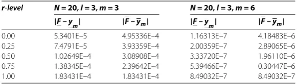
In this section, we apply the presented method in Section for solving the fuzzy integral Eq. (.) in two examples. The approximate solution is calculated for different values ofN, landm. Also, we compare the numerical solution obtained by using the proposed method with the exact solution. The computations associated with the examples were performed using Mathematica .
Example .[] Consider the following nonlinear fuzzy Fredholm integral equation:
F(t) =f(t)⊕(FR)
ts
F(s)ds,
where
k(s,t) = ts
, s,t∈[, ], f(t,r) =
t– ( –r) +
t( –r) –
t( –r)
, t,r∈[, ],
f(t,r) = t+
( –r) –
t( –r) –
t( –r)
, t,r∈[, ].
The exact solution is
F(t,r),F(t,r)=
t–
( –r),t+ ( –r)
.
The comparison of the HBT solution and the exact solution is shown in Table .
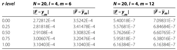
Example . Consider the following nonlinear fuzzy Fredholm integral equation:
F(t) =f(t)⊕(FR)
sexp(–t)F(s)ds,
Table 1 The accuracy on the level sets for Example 6.1 int= 0.5
r-level N = 20,l = 3,m = 3 N = 20,l = 3,m = 6
|F – y
m| |F – ym| |F – ym| |F – ym|
Table 2 The accuracy on the level sets for Example 6.2 int= 0.5
r-level N = 20,l = 4,m = 6 N = 20,l = 4,m = 12
|F – y
m| |F – ym| |F – ym| |F – ym|
0.00 2.72812E–4 3.5242E–4 5.40018E–7 7.09831E–7 0.25 2.81818E–4 3.41478E–4 5.57681E–7 6.84684E–7 0.50 2.9108E–4 3.30832E–4 5.76266E–7 6.60765E–7 0.75 3.00607E–4 3.20476E–4 5.95818E–7 6.38016E–7 1.00 3.10403E–4 3.10403E–4 6.16384E–7 6.16384E–7
where
k(s,t) =sexp(–t), s,t∈[, ], f(t,r) = cosht+exp(–t)
exp(–)
–
exp()
–
+
exp(–)r
+ r +
exp(–)r
, –
r
,
, t,r∈[, ],
f(t,r) = cosht+exp(–t)
,exp(–)
, –
exp()
–
, ,–
exp(–)r ,
– r
,+
exp(–)r
, –
r
,
, t,r∈[, ].
The exact solution in this case is given by
F(t,r),F(t,r)=
cosht+
( + r)exp(–t),cosht+
( – r)exp(–t)
.
The comparison of the HBT solution and the exact solution is shown in Table .
7 Conclusion
In this paper, we have suggested an iterative procedure by utilizing fuzzy HBT to solve the nonlinear Ferdholm fuzzy integral Eq. (.). The error estimate of the approximated function was obtained by using the fuzzy Taylor theorem [] for the function which is (i)-gH-differentiable. The error estimate of the present method is proved; for getting the best approximating solution of the equation, the numberNand the degree of the fuzzy hybrid polynomiallmust be chosen sufficiently large. The analyzed example illustrates the ability and reliability of the fuzzy HBT method for Eq. (.).
Competing interests
The authors declare that they have no competing interests.
Authors’ contributions
All authors contributed equally to the writing of this paper. All authors read and approved the final manuscript.
Author details
1Department of Mathematics, Science and Research Branch, Islamic Azad University, Tehran, Iran.2Department of Mathematics, Karaj Branch, Islamic Azad University, Karaj, Iran.
Received: 3 November 2014 Accepted: 27 January 2015
References
2. Balachandran, K, Kanagarajan, K: Existence of solutions of general nonlinear fuzzy Volterra-Fredholm integral equations. J. Appl. Math. Stoch. Anal.3, 333-343 (2005)
3. Park, JY, Han, HK: Existence and uniqueness theorem for a solution of fuzzy Volterra integral equations. Fuzzy Sets Syst.105, 481-488 (1999)
4. Subrahmanyam, PV, Sudarsanam, SK: A note on fuzzy Volterra integral equations. Fuzzy Sets Syst.81, 237-240 (1996) 5. Bede, B, Gal, SG: Quadrature rules for integrals of fuzzy-number-valued functions. Fuzzy Sets Syst.145, 359-380 (2004) 6. Bica, AM: Error estimation in the approximation of the solution of nonlinear fuzzy Fredholm integral equations. Inf.
Sci.178, 1279-1292 (2008)
7. Friedman, M, Ma, M, Kandel, A: Numerical solutions of fuzzy differential and integral equations. Fuzzy Sets Syst.106, 35-48 (1999)
8. Friedman, M, Ma, M, Kandel, A: Solutions to fuzzy integral equations with arbitrary kernels. Int. J. Approx. Reason.20, 249-262 (1999)
9. Wu, C, Song, S, Wang, H: On the basic solutions to the generalized fuzzy integral equation. Fuzzy Sets Syst.95, 255-260 (1998)
10. Abbasbandy, S, Allahviranloo, T: The Adomian decomposition method applied to the fuzzy system of Fredholm integral equations of the second kind. Int. J. Uncertain. Fuzziness Knowl.-Based Syst.14, 101-110 (2006) 11. Babolian, E, Sadeghi Goghary, H, Abbasbandy, S: Numerical solution of linear Fredholm fuzzy integral equations of
the second kind by Adomian method. Appl. Math. Comput.161, 733-744 (2005)
12. Rouhparvar, H, Allahviranloo, T, Abbasbandy, S: Existence and uniqueness of fuzzy solution for linear Volterra fuzzy integral equations proved by Adomian decomposition method. ROMAI J.5(2), 153-161 (2009)
13. Abbasbandy, S, Babolian, E, Alavi, M: Numerical method for solving linear Fredholm fuzzy integral equations of the second kind. Chaos Solitons Fractals31(1), 138-146 (2007)
14. Khezerloo, M, Allahviranloo, T, Salahshour, S, Khorasani Kiasari, M, Haji Ghasemi, S: Application of Gaussian quadratures in solving fuzzy Fredholm integral equations. In: Information Processing and Management of Uncertainty in Knowledge-Based Systems. Applications. Communications in Computer and Information Science, vol. 81, pp. 481-490 (2010)
15. Salehi, P, Nejatiyan, M: Numerical method for nonlinear fuzzy Volterra integral equations of the second kind. Int. J. Ind. Math.3(3), 169-179 (2011)
16. Mokhtarnejad, F, Ezzati, R: The numerical solution of nonlinear Hammerstein fuzzy integral equations by using fuzzy wavelet like operator. J. Intell. Fuzzy Syst. doi:10.3233/IFS-141446
17. Ziari, S, Ezzati, R, Abbasbandy, S: Numerical solution of linear fuzzy Fredholm integral equations of the second kind using fuzzy Haar wavelet. In: Advances in Computational Intelligence. Communications in Computer and Information Science, vol. 299 (2012)
18. Ezzati, R, Ziari, S: Numerical solution and error estimation of fuzzy Fredholm integral equation using fuzzy Bernstein polynomials. Aust. J. Basic Appl. Sci.5(9), 2072-2082 (2011)
19. Bica, AM, Popescu, C: Approximating the solution of nonlinear Hammerstein fuzzy integral equations. Fuzzy Sets Syst. 245, 1-17 (2014)
20. Bica, AM, Popescu, C: Numerical solutions of the nonlinear fuzzy Hammerstein-Volterra delay integral equations. Inf. Sci.223, 236-255 (2013)
21. Ezzati, R, Ziari, S: Numerical solution of nonlinear fuzzy Fredholm integral equations using iterative method. Appl. Math. Comput.225, 33-42 (2013)
22. Mirzaee, F: Numerical solution of Fredholm fuzzy integral equations of the second kind using hybrid of block-pulse-functions and Taylor series. Ain Shams Eng. J.5, 631-636 (2014)
23. Dubois, D, Prade, H: Fuzzy numbers: an overview. In: Analysis of Fuzzy Information, vol. 1, pp. 3-39. CRC Press, Boca Raton (1987)
24. Wu, C, Gong, Z: On Henstock integral of fuzzy-number-valued functions (I). Fuzzy Sets Syst.120, 523-532 (2001) 25. Bede, B, Stefanini, L: Generalized differentiability of fuzzy-valued functions. Fuzzy Sets Syst.230, 119-141 (2013) 26. Bica, AM: Algebraic structures for fuzzy numbers from categorial point of view. Soft Comput.11, 1099-1105 (2007) 27. Gal, SG: Approximation theory in fuzzy setting. In: Anastassiou, GA (ed.) Handbook of Analytic-Computational
Methods in Applied Mathematics, pp. 617-666. Chapman & Hall/CRC Press, Boca Raton (2000)
28. Stefanini, L: A generalization of Hukuhara difference and division for integral and fuzzy arithmetic. Fuzzy Sets Syst. 161, 1564-1584 (2010)
29. Congxin, W, Cong, W: The supremum and infimum of the set of fuzzy numbers and its applications. J. Math. Anal. Appl.210, 499-511 (1997)
30. Fang, J-X, Xue, Q-Y: Some properties of the space fuzzy-valued continuous functions on a compact set. Fuzzy Sets Syst.160, 1620-1631 (2009)
31. Chalco-Cano, Y, Roman-Flores, H: On new solutions of fuzzy differential equations. Chaos Solitons Fractals38, 112-119 (2008)
32. Goetschel, R, Voxman, W: Elementary fuzzy calculus. Fuzzy Sets Syst.18, 31-43 (1986)
33. Gong, Z, Wu, C: Bounded variation absolute continuity and absolute integrability for fuzzy-number-valued functions. Fuzzy Sets Syst.129, 83-94 (2002)
34. Anastassiou, GA: Fuzzy Mathematics: Approximation Theory. Springer, Berlin (2010)
35. Jung, ZH, Schanfelberger, W: Block-Pulse Functions and Their Applications in Control Systems. Springer, Berlin (1992) 36. Maleknejad, K, Mahmoudi, Y: Numerical solution of linear Fredholm integral equation by using hybrid Taylor and
Block-pulse functions. Appl. Math. Comput.149, 799-806 (2004)