R E S E A R C H
Open Access
On nonlocal boundary value problems of
nonlinear
nth-order
q-difference equations
S Phothi
*, T Suebcharoen and B Wongsaijai
*Correspondence: [email protected]
Department of Mathematics Faculty of Science, Chiang Mai University, Chiang Mai, Thailand
Abstract
In this paper, we study the existence and uniqueness of the solution of nonlocal boundary value problems of nonlinearnth-orderq-difference equations. The
uniqueness follows from the well-known Banach contraction principle. We prove that thoseq-solutions, under some conditions, converge to the classical solution whenq approaches 1–. A new numerical algorithm is introduced via definition ofq-calculus for solving the nonlocal boundary value problem of nonlinearnth-orderq-difference equations. The numerical experiments show that the algorithm is quite accurate and efficient. Moreover, numerical results are carried out to confirm the accuracy of our theoretical results of the algorithm.
1 Introduction and preliminary
Ordinary differential equations (ODEs) give a description of phenomena that change con-tinuously. They play an important role in physics, engineering and mathematics. Gener-ally, a solution of a system of ODEs is determined by specifying some conditions on some points in a domain. One of the interesting problems which arises in many subjects of phys-ical science is a boundary value problem (BVP). Specific conditions of BVPs are imposed at different values of the independent variable, for instance, consider the Robin problem
u(t) +ft,u(t),u(t)= ()
with the boundary conditions
u() = and u() = . ()
Equations () and () are commonly called ‘the local problem’. A further generalization of BVPs is those with nonlocal conditions. If we replace the conditionu() = in () by
u() =u(η), then () with the conditions
u() = and u() =u(η), ()
whereη∈(, ), is called the nonlocal problem. Note that (), () is a particular case of (), () when we have the limitη→–.
Nonlocal BVPs seem to be more interesting than the local ones not only they are more natural but also because of their numerous applications. Moreover, in the numerical ex-periment, the calculation of the value of a local boundary condition, such asu() in (), is more difficult than that of the nonlocal condition (u(η) –u())/(η– ) in (). For more information as regards nonlocal BVPs see [–] and [].
Recently, the study ofq-difference equations has played an important role in various fields of physics and mathematics, especially in quantum mechanics, due to its numerous applications. Starting from the re-introduction of theq-difference operator by Jackson [] in , the subject ofq-difference equations has been deeply studied by several authors; some examples of results can be found in [–] and [].
The existence and uniqueness of solutions ofq-difference BVPs have been studied by several authors; see [, , ]. For nonlocalq-difference problems, Ahmad and Nieto [] recently proved that a solution to the problems given by
⎧ ⎨ ⎩
Dqu(t) =f(t,u(t)),t∈[, ]q,
u() = ,Dqu() = ,u() =αu(η), ()
wheref ∈C([, ]q×R,R),η∈ {qn:n∈N}andα=η, does exist and it is unique. In this paper, for a given positive integern, we study the existence and uniqueness of the solution of the following nonlocal boundary value problem of nonlinear singularn th-orderq-difference equations:
⎧ ⎨ ⎩
Dn
qu(t) =f(t,u,Dqu, . . . ,Dmq), ≤t≤, Dk
qu() = ,u() =αu(η),k= , , , . . . ,n– ,
()
whereη∈[, ]qandmis a non-negative integer withm≤n– ,α=ηn–, andf is a con-tinuous function inC([, ]q×Rm+,R), [, ]q={qn:n∈N} ∪ {, }.
In the last section of this paper, we proceed to its numerical solution and give the com-parison with the ordinary difference equations.
2 Preliminary
In order to introduce our results, we recall some needed concepts aboutq-calculus and
q-difference equations. From now let <q< . Theq-difference operator, re-introduced by Jackson, is defined by
Dqf(t) =
f(t) –f(qt)
( –q)t , t= ;
while theq-derivative at zero is defined by
Dqf() =lim
t→Dqf(t).
Note that when the left limit asqapproaches of theq-derivative is a classical derivative
df
dt. The higher orderq-derivatives are defined inductively as
Further, for a multivariable real continuous function f(x,x, . . . ,xn), the partial q
-derivative with respect toxiis defined as
∂qf(x,x, . . . ,xn)
Also, the higher order partialq-derivative with respect toxiis defined as
∂qnf(x,x, . . . ,xn)
In , Jackson [] has generalized the so-calledq-integral, firstly introduced by Thomae [], in the following way:
t
provided that the series converges, and generally
b
binomial coefficient can be defined as
We will also use the notation
Al-Salam [] proved theq-analog of Cauchy’s formula as follows:
Iqnf(t) = t
n–
[n– ]q!
t
qs t ;q
n– f(s)dqs.
Theq-Leibniz product rule andq-integration by parts formula are
Dq(gh)(t) =Dqg(t)h(t) +g(qt)Dqh(t)
and
t
f(s)Dqg(s)dqs=f(s)g(s)t–
t
Dqf(s)g(qs)dqs,
respectively.
3 Existence and uniqueness of solutions
LetCmq be the space of all real-valued continuous functions defined on [, ]q such that
the first m q-derivatives Dqf(t),Dqf(t), . . . ,Dmqf(t) exist. We equip this space with the
norm
u q= max
≤k≤m
Dk quq,∞
, u∈Cq,m≤n– ,
where
u q,∞= max
t∈[,]q
u(t).
Lemma . Define the Green function G(t,s;q)by
G(t,s;q)
=
[n– ]q!(t–qs)
(n–)
q +
tn–[α(η–qs)(n–)
q – ( –qs)(qn–)]
–αηn– , ≤s<min{η,t};
=
[n– ]q!
tn–[α(η–qs)(n–)
q – ( –qs)(qn–)]
–αηn– , ≤t<s<η< ;
=
[n– ]q!(t–qs)
(n–)
q –
tn–( –qs)(n–) q
–αηn– , ≤η<s<t≤;
=
[n– ]q!
–t
n–( –qs)(n–) q
( –αηn–)
Then u(t)is a solution of ()if and only if of the Cauchy formula, we obtain
u(t) =
Remark . Ifqapproaches on the left, then equation () takes the form
u(t) =
G(t,s)fs,u,u, . . . ,u(m)ds, ()
with the associated form of Green’s function for the classical case defined by
G(t,s)
=
(n– )!(t–s)
n–+tn–[α(η–s)n–– ( –s)n–]
= (n– )!
tn–[α(η–s)n–– ( –s)n–]
–αηn– , ≤t<s<η< ;
=
(n– )!{(t–s)
n––tn–( –s)n–
–αηn– , ≤η<s<t≤;
=
(n– )!
–t
n–( –s)n–
–αηn–
, ≤max{η,t}<s≤. ()
This solution is equivalent to the solution of a classical nonlinear nth-order boundary value problem,
u(n)(t) =ft,u,u, . . . ,u(m), u(k)() = ,
u() =αu(η), k= , , , . . . ,n– ,m≤n– ,
()
wheref is a continuous function inC([, ]×Rm+,R).
To accomplish the main results, we define an integral operatorTq:Cm
q →Cmq by
Tqu(t) =
G(t,s;q)fs,u,Dqu, . . . ,Dmqudqs,
=
[n– ]q!
t
(t–qs)(qn–)fs,u,Dqu, . . . ,Dmqudqs
+ t
n–
[n– ]q!( –αηn–)
α
η
(η–qs)(qn–)fs,u,Dqu, . . . ,Dmqudqs
–
( –qs)(qn–)fs,u,Dqu, . . . ,Dmqudqs
.
Obviously,Tqis well defined and it is easy to see thatu∈Cm
q is a solution of BVP () if and
only ifuis a fixed point ofTq.
The following lemma will be required in our investigation.
Lemma . For k= , , . . . ,m,
DkqTqu(t) =
∂qkG(t,s;q)
∂qt
fs,u,Dqu, . . . ,Dmqudqs,
where the function∂qkG(t,s;q)/∂qt is defined by
∂k qG(t,s;q)
∂qt
=
[n–k– ]q!
(t–qs)(qn–k–)
+t
n–k–[α(η–qs)(n–)
q – ( –qs)(qn–)]
–αηn– , ≤s<min{η,t};
=
[n–k– ]q!
tn–k–[α(η–qs)(n–)
q – ( –qs)(qn–)]
=
Proof The result is directly obtained by equation ().
Lemma . For any positive integer m,we have
x
In order to state our main result, we firstly define
where
Based on Banach’s fixed point theorem [], we obtain the following result.
Theorem . Let f : [, ]q×Rm+→Rbe a continuous function,and there exist positive
Then the boundary value problem()has a unique solution,providedqGq< ,where
q=
m
j= Lj q,∞.
Proof According to the Banach contraction theorem, ifTqis a contractive mapping then it has a unique fixed point which coincides with the unique solution of problem (). To obtain the contractive property ofTq, letu,v∈Cqmand for eacht∈Iq, we have
Theorem . Let f : [, ]×Rm+→Rbe a continuous function,and there exist positive functions Lj(t)∈C([, ]),j= , , . . . ,m,such that
f(t,u,u, . . . ,um) –f(t,v,v, . . . ,vm)≤ m
j=
Lj(t)|uj–vj|, t∈[, ]. ()
Then the boundary value problem()has a unique solution,providedG< ,where=
m
j= Lj ∞andG=limq→–Gq.
4 Numerical experiments
In this section, we prove the error estimate between theq-difference solution and the classical solution. Letuqbe the solution of () andube the solution of (). We note here
that, for any functionf: [, ]×Rm+→Rin problem (), for convenience its restriction f|[,]q×Rm+will be written asf when we consider problem (), similarly to the functionu, so that u–uq q,∞is well defined.
Theorem . Let f : [, ]×Rm+→Rbe a continuous function satisfying the Lipschitz condition().Ifmax{qGq,G}< ,then
u–uq q,∞≤ Tu–Tqu q,∞+
G
–G Tu–u ∞+ qGq
–qGq
Tqu–u q,∞. ()
Moreover,if u=u,we have
u–uq q,∞≤
–qGq
Tu–Tqu q,∞. ()
Proof To prove the error estimate, the following bounds are valid by Theorem . and Theorem .:
Tqnu–uq∞≤
(qGq)n
–qGq
Tqu–uq q,∞,
Tnu–u∞≤
(G)n
–G Tu–u ∞,
respectively. It is easy to see that
Tnu–uq,∞≤Tnu–u∞.
Thus, we have
u–uq q,∞≤Tnu–uq,∞+Tnu–Tqnuq,∞+Tqnu–uqq,∞
≤ (G)n
–G Tu–u ∞+T
nu
–Tqnuq,∞
+ (qG)
n
–qG
Considering the middle term Tnu
This completes the proof.
Next, we will apply theq-Picard iterative method to solve someq-nonlinear boundary value problems and compare the approximate solutions with their exact solutions. In order to identify the method, we first establish the correctional function for () as
×
α
η
(η–qs)(qn–)fs,un(s), . . . ,Dmqun(s)dqs
–
( –qs)(qn–)fs,un(x), . . . ,Dmqun(s)dqs
, ()
whereunrepresents thenth-order approximate.
Starting from the initial iterationu(t), the successive approximate solutions can be
ob-tained by calculating theq-integral appeared in (). Occasionally, it might be difficult to calculate theq-integration directly due to the nonlinearity off(t,·).
Now we shall present the explicit algorithm for solving an approximate solution of the
q-integral via operatorTqdefined above. Letq¯Nbe the time scale which given as{qn|n∈ N} ∪ {}, where is the cluster point ofq¯N. For the numerical computations, the interval [,q] is partitioned intoNsubintervals. Recall that the analog maximum errors are defined as
un–u∗L∞=max
t∈Iq
un(t) –u∗(t),
whereunis the approximate solution withniterations andu∗is the analytic solution.
Recall that theq-derivative ofun(t) att=qjis defined as
Dqun
qj=un(q
j) –un(qj+)
( –q)qj , j= , , . . . ,N– ,
and hence the boundary condition gives
DqunqN=un(q
N) –un(qN+)
( –q)qN ≈
un(qN)
( –q)qN,
where we useun(qN+)≈. By the inductive step, we obtain
Dkqunqj=D
k–
q un(qj) –Dqk–un(qj+)
( –q)qj , j= , , . . . ,N– ,
and
Dkqun
qN=D
k– q un(qN)
( –q)qN ,
fork= , , . . . ,n– . In the casek=n– , then– times derivative ofun(t) att= can be defined by
Dnq–un() = lim
j→∞
Dnq–un(qj) –Dnq–un()
qj , q< . ()
Then we can estimateDn– q un() =
Dnq–un(qN–)
We can calculate theu(qk) =Tu(qk), wherek= , , , . . . ,N– , and we have the
quan-Similarly, the following estimations are obtained:
By using the values ofuk–(t), for allt∈[, ]q, we can repeatedly calculate theuk(t), for k= , , . . . ,n. Next, we present two numerical experiments to illustrate the efficiency of the proposed algorithm. The computer programs are written in MATLAB by choosing
N= ,.
Example . Let us first consider theq-difference BVP
⎧ ⎨ ⎩
D
qu=[]qt[]qDqu–
t []qu+ –
qt []q[]q,
u() = ,u() =u(q),
withf(t,u,Dqu) =[]t
q[]qDqu–
t []qu+ –
qt
[]q[]q,n= ,α= andη=q.
Clearly
f(t,v,v) –f(t,w,w)≤ t
[]q[]q|
v–w|+ t
[]q| v–w|,
for <q< , we chooseq= /[]q[]q+ /[]q< ,C= /[]q andγ = ( –q)/( –q) =
[]q. Then we have
Gq=max
,| –γC|
= .
By using Theorem ., we only can obtain the existence and uniqueness of solution of problem (.), however, it is not difficult to show this, and the exact solution is u(t) =
t []q –t.
Withu= andN= , we apply the numerical schemes for solving this problem.
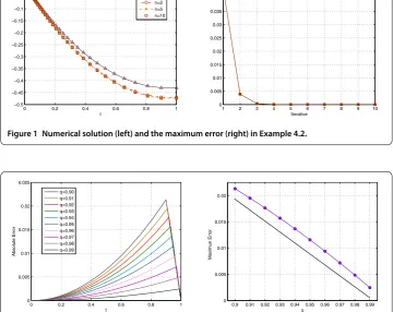
Ta-ble shows the errors forq= ., ., ., . at the various values of iteration. It seems that the approximationunconverges faster whenqis large. Figure presents theq-approximate
Table 1 Numerical comparison of the errors in Example 4.2
n q
0.6 0.7 0.8 0.9
1 5.14630E–02 5.03004E–02 4.73555E–02 4.34192E–02
2 6.99387E–03 6.04295E–03 4.93923E–03 3.89799E–03
3 9.43402E–04 7.16415E–04 5.04360E–04 3.38723E–04
4 1.27086E–04 8.47161E–05 5.13017E–05 2.93003E–05
5 1.71157E–05 1.00129E–05 5.21482E–06 2.53324E–06
6 2.30502E–06 1.18335E–06 5.30033E–07 2.19010E–07
7 3.10421E–07 1.39850E–07 5.38716E–08 1.89344E–08
8 4.18050E–08 1.65275E–08 5.47540E–09 1.63698E–09
9 5.62994E–09 1.95323E–09 5.56510E–10 1.41532E–10
10 7.58194E–10 2.30834E–10 5.65640E–11 1.22410E–11
11 1.02108E–10 2.72809E–11 5.74957E–12 1.06670E–12
12 1.37516E–11 3.22392E–12 5.85199E–13 9.96425E–14
13 1.85246E–12 3.81251E–13 6.02296E–14 1.83742E–14
14 2.49800E–13 4.51861E–14 6.55032E–15 8.43769E–15
15 3.42504E–14 6.10623E–15 1.72085E–15 8.32667E–15
16 4.88498E–15 1.05471E–15 1.55431E–15 8.32667E–15
17 8.88178E–16 7.21645E–16 1.55431E–15 8.32667E–15
18 4.44089E–16 6.10623E–16 1.55431E–15 8.32667E–15
19 3.33067E–16 6.10623E–16 1.55431E–15 8.32667E–15
Figure 1 Numerical solution (left) and the maximum error (right) in Example 4.2.
Figure 2 The absolute error (left) and the maximum error (right) in Example 4.2.
Table 2 Comparison of the error betweenq-approximate solutionu15and classical ODE
q 0.900 0.925 0.950 0.975
u15–u q,∞ 2.13158E–02 1.15705E–02 7.16421E–03 2.46256E–03
solution for the different values ofnon the left side and it presents the maximum error on the right side withq= ..
In Figure , the absolute errors with several values ofq and the maximum errors are plotted withn= . Furthermore, we also compute the error betweenq-approximate so-lution,u, and the exact solution obtained by the classical ODE; the results are shown in
Table .
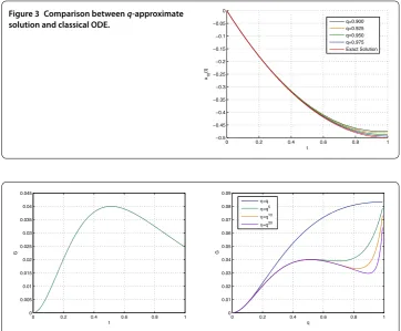
Finally, Figure presents theq-approximate solution with several values ofqand exact solution of the classical ODE in Example ..
Example .([]) Consider the BVP
⎧ ⎨ ⎩
D
qu=L(cost+tan–u),
u() =Dqu() = andu() =αu(qk),
Figure 3 Comparison betweenq-approximate solution and classical ODE.
Figure 4 Plots of the functionGwithα= 0 (left) andα= 1 (right).
We find that
f(t,u) –f(t,v)≤Ltan–u–tan–v≤L|u–v|.
We shall show that the BVP has a unique solution. We haveq=LandC= /[]qso
that
Gq=max
|α|qk( –qk)
| –αqk|( +q)( +q+q),
|γ|( +q)q
( +q+q)
=|γ|
( +q)q
( +q+q).
Hereγ = ( –qk)/( –qk).
We can roughly estimate that
Gq<
+qk
( +q+q).
So, this problem has a unique solution providedL<(+q+q)
+qk .
Some examples of the functionGqare shown in Figure withα= on the left andα=
on the right. In these cases, it is observed that we have the maximum values ofGq< .
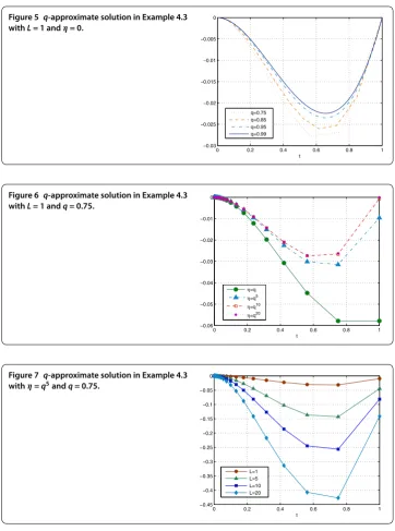
Figure 5 q-approximate solution in Example 4.3 withL= 1 andη= 0.
Figure 6 q-approximate solution in Example 4.3 withL= 1 andq= 0.75.
Figure 7 q-approximate solution in Example 4.3 withη=q5andq= 0.75.
existence and uniqueness of problem ., however, we cannot obtain its exact solution. Hence, we will apply the numerical scheme to obtain its numerical solution.
Figure presents theq-approximate solution with several values ofqforL= andη= . Moreover, theq-approximate solution with several values ofηandLare displayed in Fig-ure and FigFig-ure , respectively.
Competing interests
The authors declare that they have no competing interests.
Authors’ contributions
Acknowledgements
This research was financially supported by Chiangmai University.
Publisher’s Note
Springer Nature remains neutral with regard to jurisdictional claims in published maps and institutional affiliations.
Received: 18 January 2017 Accepted: 11 May 2017
References
1. Guo, Y, Ji, Y, Zhang, J: Three positive solutions for a nonlinearnth-order -point boundary value problem. Nonlinear Anal.68(11), 3485-3492 (2008)
2. Eloe, PW, Ahmad, B: Positive solutions of a nonlinearnth order boundary value problem with nonlocal conditions. Appl. Math. Lett.18(5), 521-527 (2005)
3. Sun, Y: Positive solutions for third-order three-point nonhomogeneous boundary value problems. Appl. Math. Lett.
22(1), 45-51 (2009)
4. Han, X: Positive solutions for a three-point boundary value problem at resonance. J. Math. Anal. Appl.336(1), 556-568 (2007)
5. Liu, B: Positive solutions of a nonlinear three-point boundary value problem. Comput. Math. Appl.44(1-2), 201-211 (2002)
6. Jackson, FH: Onq-functions and a certain difference operator. Trans. R. Soc. Edinb.46, 253-281 (1908) 7. Jackson, FH:q-difference equations. Am. J. Math.32(4), 305-314 (1910)
8. Carmichael, RD: The general theory of linearq-difference equations. Am. J. Math.34(2), 147-168 (1912)
9. El-Shahed, M, Hassan, HA: Positive solutions ofq-difference equation. Proc. Am. Math. Soc.138(5), 1733-1738 (2010) 10. Dobrogowska, A, Odzijewicz, A: Second orderq-difference equations solvable by factorization method. J. Comput.
Appl. Math.193(1), 319-346 (2006)
11. Trjitzinsky, WJ: Analytic theory of linearq-difference equations. Acta Math.61(1), 1-38 (1933)
12. Mason, TE: On properties of the solutions of linearq-difference equations with entire function coefficients. Am. J. Math.37(4), 439-444 (1915)
13. Ahmad, B, Nieto, J: On nonlocal boundary value problems of nonlinearq-difference equations. Adv. Differ. Equ.2012, 81 (2012)
14. Ahmad, B, Ntouyas, SK, Purnaras, IK: Existence results for nonlocal boundary value problems of nonlinear fractional q-difference equations. Adv. Differ. Equ.2012, 140 (2012)
15. Jackson, FH: Onq-definite integrals. Q. J. Pure Appl. Math.41, 193-203 (1910)
16. Thomae, J: Ueber die höheren hypergeometrischen Reihen, insbesondere über die Reihe: 1 +a0a1a2
1.b1b2x+
a0 (a0 +1)a1 (a1 +1)a2 (a2 +1) 1.2.b1 (b1 +1)b2 (b2 +1) x
2+· · · ·. Math. Ann.2(3), 427-444 (1870) 17. Al-Salam, WA:q-analogues of Cauchy’s formulas. Proc. Am. Math. Soc.17, 616-621 (1966)