An optimized Crank–Nicolson finite difference extrapolating model for the fractional order parabolic type sine Gordon equation

(1)

R E S E A R C H

Open Access

An optimized Crank–Nicolson ﬁnite

difference extrapolating model for the

fractional-order parabolic-type sine-Gordon

equation

Yanjie Zhou

1

_{and Zhendong Luo}

2*

*_{Correspondence:}_{[email protected]}

2_{School of Mathematics and}

Physics, North China Electric Power University, Beijing, China Full list of author information is available at the end of the article

Abstract

In this paper, by means of a proper orthogonal decomposition (POD) we mainly reduce the order of the classical Crank–Nicolson finite difference (CCNFD) model for the fractional-order parabolic-type sine-Gordon equations (FOPTSGEs). Toward this end, we will first review the CCNFD model for FOPTSGEs and the theoretical results (such as existence, stabilization, and convergence) of the CCNFD solutions. Then we establish an optimized Crank–Nicolson finite difference extrapolating (OCNFDE) model, including very few unknowns but holding the fully second-order accuracy for FOPTSGEs via POD. Next, by a matrix analysis we will discuss the existence,

stabilization, and convergence of the OCNFDE solutions. Finally, we will use a numerical example to validate the validity of theoretical conclusions. Moreover, we show that the OCNFDE model is very valid for settling FOPTSGEs.

MSC: 34K28; 35R11; 65M12

Keywords: Proper orthogonal decomposition; Classical Crank–Nicolson finite difference model; Fractional-order parabolic-type sine-Gordon equation; Optimized Crank–Nicolson finite difference extrapolating model; Existence, stabilization, and convergence

1 Introduction

Though there are lots studies for fractional-order differential equations in recent years (see, e.g., [1–4]), there are few reports about the reduced-order study for the fractional-order differential equations except for Ref. [4]. In this paper, by means of proper orthogo-nal decomposition (POD) we mainly reduce the order of the classical Crank–Nicolson fi-nite difference (CCNFD) model for the fractional-order parabolic-type sine-Gordon equa-tions (FOPTSGEs) as follows.

∂ϑ(t,x)

∂t =K

∂ν_ϑ₍_t_,_x₎ ∂|x|ν +sin

ϑ(t,x), (t,x)∈(0,T)×(0,L), (1)

ϑ(t, 0) =ϑ(t,L) =g(t), t∈(0,T), (2)

ϑ(0,x) =ϕ(x), x∈(0,L), (3)

(2)

where K is the known coeﬃcient of dispersion, 1 <ν≤2,T is the total time, Lis the positive real number, g(t) is a known boundary value function, ϕ(x) is a known initial function, and∂ν_ϑ₍_t_,_x_)/_∂_|_x_|ν_{is the fractional-order derivative, deﬁned by}

∂ν_ϑ₍_t_,_x₎ ∂|x|ν =S(ν)

∂2 ∂x2

x

0

(x–y)1–νϑ(t,y) dy+ L

x

(y–x)1–νϑ(t,y) dy

, (4)

whereS(ν) = –[2cos(νπ

2)Γ(2 –ν)]–1andΓ(·) is the Gamma distribution function. For

sim-plicity we further suppose thatg(t) = 0 in the following discussion.

The FOPTSGEs (1)–(3), which are substantially parabolic-type fraction-order par-tial differenpar-tial equations (PDEs) with the nonlinear term sin(ϑ), just as the standard fractional-order PDEs in [5–7], also hold very important physical meanings, such as phe-nomena in fluid dynamics in porous media, groundwater dynamics, and seepage hy-draulics groundwater hyhy-draulics (see, e.g., [2,3,5,6]). Nevertheless, the FOPTSGEs (1)– (3) usually have no analytic solution, so that we have to rely on numerical methods (see, e.g., [6,7]). Recently, a CCNFD model of the FOPTSGEs (1)–(3) has been established in [8], but it contains a lot of unknowns (i.e., degrees of freedom). Therefore, because of the accumulation of the round-off error in the numerical computations, there would appear floating point overflow after a number of computing steps, so that we cannot obtain per-fect conclusions. Thus, ensuring that the CCNFD solutions hold the desired accuracy, how to reduce the unknowns of the CCNFD model so as to alleviate the calculated load and the accumulation of the round-off errors in the numerical computations is an urgent problem, which is the main mission in this paper.

POD is regarded as a valid method to reduce the order of numerical models (see [9– 12]). It substantially seeks an orthonormal basis from the given data. POD may immensely lessen the unknowns in the numerical formats and has been widely applied in many fields including pattern and signal recognition (see [13]), statistics (see [14]), and hydrodynamics (see [15]). Recently, it has been resoundingly used to the order reduction of the Galerkin, finite element, FD, finite volume element, reduced basis, and meshless methods for PDEs (see, e.g., [16–30]). Nevertheless, the existing most reduced-order models (see, e.g., [9– 30]) they are formed with the POD basis produced from the classical numerical solutions at all nodes of time, before repetitively calculating the optimized solutions at the same nodes of time, which are actually some repetitive computations. To eliminate the tauto-logical computations, some optimized FD extrapolating models based on POD have been proposed (see, e.g., [31–34]).

Nevertheless, as far as we know, there has not been any research on the optimized Crank–Nicolson finite difference extrapolating (OCNFDE) scheme of FOPTSGEs con-structed by POD. Therefore, in this paper, by POD we build the OCNFDE model only including few unknowns for FOPTSGEs. Specially, we merely choose the CCNFD solu-tions at the first several nodes of time to form the snapshots, and then use them to produce a set of POD basis, finally use the POD basis to establish the OCNFDE model for finding the OCNFDE solutions at total nodes of time. This is the same thing as utilizing the ex-isting information (on the quite short time interval [0,T0],T0T) to forecast the future

physical law (on the time interval [T0,T]). Moreover, we will adopt the error estimates to

(3)

The remaining contents of this paper are arranged as follows. In Sect.2, we first recall the CCNFD model for the FOPTSGEs (1)–(3) and extract the snapshots from the first few CCNFD solutions. In Sect.3, we produce a set of POD basis with the snapshots and set up the OCNFDE model. Then, in Sect.4, by the matrix analysis, we analyze the exis-tence, stabilization, and convergence for the OCNFDE solutions and offer the flowchart of settling the OCNFDE model. Next, in Sect.5, we use two numerical examples to verify that the conclusions of numerical calculations are accorded with the theory ones. It is also shown that the OCNFDE model is very valid for settling the FOPTSGEs (1)–(3), since it can vastly lessen the number of unknowns, alleviate the calculated load, and save the CPU consumption time and the memory space in the numerical computations. Section6finally summarizes the dominating conclusions.

2 The CCNFD model for FOPTSGEs

In this section, we review the CCNFD model for the FOPTSGEs (1)–(3), which has been posed in [8].

LetMandNrepresent two positive integers, leth=L/Mdenote the spatial step, and let

τ =T/Ndenote the time step. The CCNFD model with the fully second-order accuracy

for the FOPTSGEs (1)–(3) is denoted as follows:

(4)

Put

Therefore, the CCNFD model (5)–(6) can be presented in the following matrix format:

¯

Furthermore, the vector-format CCNFD model (7)–(8) can be reduced as follows:

Vn=Vn–1+1

Apparently, there is a unique set of the solution vector {Vn}N

n=1 for the vector-format

CCNFD model (9). The following stabilization and convergence of the set of the solution

{Vn_}N

n=1has been proved in [35, Theorem 2].

Theorem 2 AsI+E_∞≤1,the set of solution{Vn}N

n=1for the CCNFD model(9)is sta-ble and convergent.Furthermore,the error estimates between the set of solution{Vn_}N

n=1 for the CCNFD model(9)andV˜(tn) = [ϑ(tn,x1),ϑ(tn,x2), . . . ,ϑ(tn,xM–1)]T(n= 1, 2, . . . ,N) produced from the analytic solution of the FOPTSGEs(1)–(3)are denoted by

(5)

(lN) in the set of solution {Vn}N_n₌₁ for the CCNFD model (9) as a group of snap-shots.

3 The OCNFDE model for FOPTSGEs

3.1 Production and results of POD basis

To the snapshotsV1,V2, . . . ,Vl (lN) obtained in Sect.2, letBϑ = (V1,V2, . . . ,Vl) (ap-parentlyBϑ∈R(M–1)×l_{), let}_λ

j> 0 (j= 1, 2, . . . ,r=:rank(Bϑ)) be the positive eigenvalues of

BϑBTϑ arranged nonincreasingly, and letVϑ= (φ1,φ2, . . . ,φr)∈R(M–1)×rbe the orthonor-mal eigenvectors ofBϑBTϑ associated with the positive eigenvalues. Thus, a set of POD

basisΨ =: (φ₁,φ₂, . . . ,φ_d) (d≤r) is obtained from the initialdeigenvectors inVϑ and

holds the following result (see, e.g., [20,21,36]):

Bϑ–Ψ ΨTBϑ_2,2=λd+1, (12)

whereBϑ2,2=supx∈RM–1Bϑx2/x2, andx2is thel2norm for the vectorx∈RM–1.

Furthermore, we have

Vn–Ψ ΨTVn

2=Bϑ–Ψ Ψ

T_Bϑ_εn

2

≤Bϑ–Ψ ΨTBϑ_2,2εn₂

≤λd+1, n= 1, 2, . . . ,l, (13)

whereεn(n= 1, 2, . . . ,l) represent a set of unit orthogonal vectors withnth component being 1. Thus,Ψ = (φ₁,φ₂, . . . ,φ_d) forms a set of POD basis.

Remark4 Because the orderlof the matrixAT

ϑAϑis far smaller than the orderM– 1 of the

matrixAϑAT_ϑ, that is, the number of the snapshotslis far smaller than that of the spatial internal nodesM– 1, whereas both positive eigenvaluesλi (i= 1, 2, . . . ,r) are the same, we may ﬁrst ﬁnd the eigenvectorsψ_iand the eigenvaluesλi(i= 1, 2, . . . ,r) ofATϑAϑ, and

then compute the eigenvectorsϕ_iofAϑATϑ via the formulaϕi=Aϑψi/

√

λi(i= 1, 2, . . . ,r),

so that the POD basis can be obtained expediently.

3.2 The OCNFDE model of the FOPTSGEs

From Sect.3.1we have obtained the ﬁrstlOCNFDE solutionsVn_d=Ψ ΨTVn=:Ψ βn_d(n= 1, 2, . . . ,l≤N), whereVn_d= (un

d,1,und,2, . . . ,und,M–2,und,M–1)Tandβ

n

d= (β1n,β2n, . . . ,βdn)T. At the moment, replacing Vn_{in (9) with} _Vn

d=Ψ β n

d (n=l+ 1,l+ 2, . . . ,N), we can obtain the following OCNFDE model:

⎧ ⎪ ⎪ ⎪ ⎪ ⎪ ⎨ ⎪ ⎪ ⎪ ⎪ ⎪ ⎩

Ψ βn_d=Ψ ΨTVn_, _n_{= 1, 2, . . . ,}_l_;

Ψ βn_d=Ψ βn_d–1+1₂E(2Ψ β_dn–1+EΨ β_dn–1+τG(Ψ βn_d–1))

+τ 2[G(Ψ β

n–1

d ) +G(Ψ βdn–1+EΨ βdn–1+τG(Ψ βnd–1))], l+ 1≤n≤N,

Vn_d=Ψ βn_d, n= 1, 2, . . . ,N,

(6)

whereVn(n= 1, 2, . . . ,l) are the given CCNFD solution vectors for the CCNFD model (9). The OCNFDE model (14) is reduced to the following model:

⎧ ⎪ ⎪ ⎪ ⎪ ⎪ ⎨ ⎪ ⎪ ⎪ ⎪ ⎪ ⎩

βn_d=ΨT_ϑVn, 1≤n≤l;

βn_d=βn_d–1+₂1ΨTE[2Ψ β_dn–1+EΨ β_dn–1+τG(Ψ βn_d–1)]

+τ 2Ψ

T_[_G₍_{Ψ β}n–1

Vn_d=Ψ βn_d, 1≤n≤N.

(15)

Remark5 Since the CCNFD model (9) includes (M– 1) unknowns at each node of time, but the OCNFDE model (15) at the same node of time has onlydunknowns (dM– 1), the OCNFDE model (15) is far superior to the CCNFD model (9).

4 The existence, stabilization, and convergence for the OCNFDE solutions and the ﬂowchart for settling the OCNFDE model

4.1 The existence, stabilization, and convergence for the OCNFDE solutions

Apparently, there is a unique set of the solution vector{Vn_d}N_n₌₁for the OCNFDE model (15). Further, the stabilization and convergence for the OCNFDE solutions have the fol-lowing result.

Theorem 6 Under the same conditions of Theorem2,the series of solutions{Vn_d}N n=1of the OCNFDE model(15)is stable and convergent and has the following error estimates:

Vn–Vn_d_∞≤ρ(n)λd+1, n= 1, 2, . . . ,N, (16)

the above Vi (i = 1, 2, . . . ,N) represents the CCNFD solution vectors of the CCNFD model (9), ρ(n) = 1 (1 ≤n≤ l), and ρ(n) = (1 + 2τ +τ2)n–l ₍_l_{+ 1} _≤_n _≤_N_).

Fur-thermore, we have the error estimates between the analytic solution vectors V˜(tn) = [u(tn,x1),u(tn,x2), . . . ,u(tn,xM–1)]T(n= 1, 2, . . . ,N)of the FOPTSGEs(1)–(3)and the OC-NFDE solutionsVn_dof the OCNFDE model(15)as follows:

V˜n–Vn_d_∞≤Cτ2+h2+ρ(n)λd+1

, n= 1, 2, . . . ,N, (17)

where C is a generic positive constant.

Proof (1)The stabilization and convergence of the OCNFDE solutions ByVn

d=Ψ β n

d(n= 1, 2, . . . ,N) we can restore the OCNFDE model (14) as follows:

Vn_d=Ψ ΨTVn, 1≤n≤l; (18)

Vn_d=Vn_d–1+1 2E

2Vn_d–1+EV_dn–1+τGVn_d–1

+τ 2

GVn_d–1+GVn_d–1+EV_dn–1+τGVn_d–1, l+ 1≤n≤N. (19)

As the CCNFD solutions Vn ₍_n_{= 1, 2, . . . ,}_l_{) are given and stable, the stabilization of}_Vn d (n= 1, 2, . . . ,l) can obtained byVn

(7)

AsI+E_∞≤1, we obtain

Using the diﬀerential mean value theorem, we have

GV(ti)

–GVi_∞≤V(ti) –Vi_∞, (21)

GVi_∞≤Vi_∞. (22)

Hence, by (20)–(22) from (9) we have

Vn_d_∞≤Vn_d–1+1

which shows that the OCNFDE solutions{Vn

d}Nn=l+1are stable and convergent according to

the Lax stabilization theorem (see [10]). Therefore, the solutions{Vn

d}Nn=1for the OCNFDE

(8)

(2)The error estimates(11)of the CCNFD solutions{Vn_d}N_n₌₁

Asn= 1, 2, . . . ,l, by the properties of norm and (13) we straight-away obtain the error estimations:

Vn–Vn_d_∞≤Vn–Vn_d 2=V

n_–_{Ψ Ψ}T_Vn

2≤

λd+1, 1≤n≤l. (25)

Leten=Vn–Vnd. By subtracting (19) from (9) we get

en=en–1+

1 2E

2en–1+Een–1+τG

Vn–1–τGVn_d–1

+τ 2

GVn–1+GVn–1+EVn–1+τGVn–1

–GVn_d–1–GV_dn–1+EVn_d–1+τGVn_d–1

=τ 2

GVn–1+EVn–1+τGVn–1

–GVn_d–1+EV_dn–1+τGVn_d–1+

I+E+1 2E

2

en–1

+τ 2(I+E)

GVn–1–GV_dn–1, l+ 1≤n≤N. (26)

Thus, by (20)–(22), from (26), we have

en∞≤I+E+1

2E

2

∞

en–1∞+τ

2E∞en–1∞ +τ

2

e_n_–1_∞+I+E_∞e_n_–1_∞+τe_n_–1_∞

≤(1 +βτ)en–1∞

≤1 + 2τ+τ2e_n_–1_∞, n=l+ 1,l+ 2, . . . ,N. (27)

Thus, by iterating (27), and using (25), we have

e_n_∞≤1 + 2τ+τ2n–le_l_∞

≤1 + 2τ+τ2n–lλd+1, n=l+ 1,l+ 2, . . . ,N. (28)

Combining (25) with (28) yields (16), and combining Theorem2with (16) yields (17). This

ﬁnishes the proof of Theorem6.

Remark7 The error terms√λd+1andρ(n) = (1 + 2τ+τ2)n–l(l+ 1≤n≤N) in Theorem6

(9)

to zero. Thus, if we selectd that satisﬁes (1 + 2τ +τ2₎N–l√_λ

d+1≤min{τ2,h2}, then we

can ensure that the OCNFDE solutions reach the optimal convergence order, i.e., when we selectdthat satisﬁes (1 + 2τ+τ2₎N–l√_λ

d+1≤min{τ2,h2}, the OCNFDE solutions have

second-order accuracy.

4.2 Flowchart of settling the OCNFDE model

The ﬂowchart for settling the ROESTCFE model of the FOPTSGEs (1)–(3) consists of the following six steps.

Step 1Extract the snapshotsVi ₍_i_{= 1, 2, . . . ,}_l_{, usually}_l_{= 20) from the ﬁrst}_l_CCNFD solutions of the CCNFD model:

Vn=Vn–1+1 2E

2Vn–1+EVn–1+τGVn–1

+τ 2

GVn–1+GVn–1+EVn–1+τGVn–1, n= 1, 2, . . . ,l,

satisfying the following initial value conditions:

V0=ϑ₁0,ϑ₂0, . . . ,ϑ_M0_–2,ϑ_M0_–1T, ϑ_i0=ϕ(0,ih),i= 1, 2, . . . ,M– 1.

Step 2Form the snapshot matrixAϑ= [V1,V2, . . . ,Vl].

Step 3Compute the eigenvaluesλ1≥λ2≥ · · · ≥λr> 0 and the corresponding eigenvec-torsψj(j= 1, 2, . . . ,r=:dim{V1_,_V2_{, . . . ,}_Vl_}_{) of the matrix}_AT

ϑAϑ.

Step 4 For the given time stepτ and spatial stephand the desired error boundδ= O(τ2,h2), choose the numberdof the POD basis that satisﬁesλd+1≤δ2.

Step 5Formulate the POD basisΨ = [ϕ₁,ϕ₂, . . . ,ϕ_d] byϕ_i=Aϑψ_i/√λi(i= 1, 2, . . . ,d) and obtain the OCNFDE solutions by settling the OCNFDE model:

⎧ ⎪ ⎪ ⎪ ⎪ ⎪ ⎨ ⎪ ⎪ ⎪ ⎪ ⎪ ⎩

βn_d=ΨT_ϑVn, 1≤n≤l;

βn_d=βn_d–1+₂1ΨTE(2Ψ β_dn–1+EΨ β_dn–1+τG(Ψ βn_d–1))

+τ 2Ψ

T_[_G₍_{Ψ β}n–1

Vn_d=Ψ βn_d, 1≤n≤N,

which only containsdunknowns.

Step 6On condition that (1 + 2τ+τ2)n–l√λd+1=O(τ2,h2) (n=l+ 1,l+ 2, . . . ,N), then

end; else, letVi=Vn_d–l–i(i= 1, 2, . . . ,l), then return to Step 2.

5 Two numerical examples

In this following, we oﬀer two numerical examples to explain that the advantage of the OCNFDE model (15) of the FOPTSGEs (1)–(3).

5.1 The comparison between the OCNFDE and CCNFD solutions

In the FOPTSGEs (1)–(3), we chooseT= 2000 (i.e., 0≤t≤2000),L= 16,000 (i.e., 0≤x≤ 16,000),τ=h= 0.01,K= 1,ν= 1.5, the boundary valueg(t) = 0.22, and the initial function

u(0,x) =ϕ(x) = ⎧ ⎨ ⎩

0.22 +sin(πx/2000), x∈[6000, 8000],

(10)

Under this case, it is not easy to seek the analytical solution of the FOPTSGEs (1)–(3), so that we have to rely on the numerical solutions.

We first find the firstl= 20 solution vectorsVn(n= 1, 2, . . . , 20) by the CCNFD model (9) and form the snapshot matrixBϑ= [V1,V2, . . . ,V20]. Then by Steps 3 and 5 in Sect.4.2

we ﬁnd the eigenvaluesλ1≥λ2≥ · · · ≥λ20≥0 and the corresponding eigenvectors ϕj (j= 1, 2, . . . , 20). By estimating we gain that√λ7≤3.5×10–4. Thus, we choose the POD

basisΨ = [ϕ₁,ϕ₂, . . . ,ϕ₆] and compute the OCNFDE solutionsϑ_din (n= 1, 2, . . . , 200,000 andi= 1, 2, . . . , 1,600,000, i.e., 0 <t≤2000 and 0≤x≤16,000) via the OCNFDE model (15), and depict them graphically in Fig.1. To compare with the OCNFDE solutions, we also ﬁnd the CCNFD solutionsϑ_in(n= 1, 2, . . . , 200,000 andi= 1, 2, . . . , 1,600,000, i.e., 0 < t≤2000 and 0≤x≤16,000) via the CCNFD model (9), and depict them graphically in Fig.2. Although Fig.2and Fig.1are almost the same, by carefully comparing we ﬁnd that the conclusions of the OCNFDE solutions in Fig.1are better than those of the CCNFD solutions in Fig.2.

Figure 1The ROENBE solutions when 0≤t≤2000 and 0≤x≤16,000

(11)

Figure 3The error photo between the CCNFD solutions and the OCNFDE solutions on 0≤t≤2000

Table 1 Comparisons of errors and CPU time of the CCNFD and OCNFDE solutions

Real time CCNFD scheme OCNFDE scheme

Error ˜V(tn) –Vn2 CPU time Error ˜V(tn) –Vn_d2 CPU time

n= 100,000 0.00046 381 s 0.00048 3.0 s

n= 150,000 0.00058 571 s 0.00063 4.5 s

n= 200,000 0.00076 762 s 0.00082 6.0 s

Figure3shows the error photo between the CCNFD solutions and the OCNFDE solu-tions on 0≤t≤2000, which accords with the theoretical conclusion of (16) in Theorem6, since both the theoretical and the numerical errors areO(10–4) asτ=h= 0.01.

As the CCNFD model at each node of time includes 1,600,000 unknowns, but the OC-NFDE model at the same node of time only contains six unknowns, the OCOC-NFDE model can immensely alleviate the accumulation of the round-oﬀ error in the numerical compu-tation and enhance the accuracy of the OCNFDE numerical solutions. From the records for settling the CCNFD model and the OCNFDE model in the same Laptop (iPone Mac book: Int Core i5 Processor, 16 GB RAM) we ﬁnd that the CPU consumption time for set-tling the CCNFD model on 0≤t≤2000 is 762 min, whereas the CPU consumption time for settling the OCNFDE model is less than 6 min, that is, the CPU consumption time for settling the CCNFD model is 126 times more than that for settling the OCNFDE model. More comparisons of errors and CPU time of the CCNFD and OCNFDE solutions are listed in Table1, where ˜V(tn) –Vn2and ˜V(tn) –Vnd2are approximately estimated by

Vn+1–Vn2andVnd+1–Vnd2, respectively.

Table1further shows that the numerical computing conclusions accord with the theo-retical ones. This implies that the OCNFDE model is eﬀective for settling the FOPTSGEs (1)–(3) and that the OCNFDE model is far superior to the CCNFD model.

5.2 The comparison between the OCNFDE method and OCNFDE/DEI method

When we solve the OCNFDE model (15), we need to compute the following nonlinear terms:

GPODβ_dn–1=:ΨTGΨ βn_d–1,

(12)

for solving the OCNFDE model (15), we adopt a discrete-empirical-interpolation (EDI) method for the nonlinear termsG(Ψ βn_d–1), i.e., the nonlinear termsG(Ψ βn_d–1) are approx-imated with the EDI termsGEDIas follows:

GPODβ_dn–1GEDIβ_dn–1=:ΨTGˆPTGˆ–1PTGΨ βn_d–1,

where Gˆ ∈R(M–1)×d _{contains the ﬁrst}_d _{POD bases produced by the snapshots} _G₍_Vn₎ (n= 1, 2, . . . ,L) associated with the largestdeigenvalues,P= [eρ₁,eρ₂, . . . ,eρ_d]∈R(M–1)×d consists of the rows ofGcorresponding to the DEIM indicesρ1,ρ2, . . . ,ρdthat are obtained by the greedy algorithm (see [29,39]).

In the second example, we chooseT = 2.5 (i.e., 0≤t≤2.5),L= 2.7 (i.e., 0≤x≤2.5),

τ =h= 0.01,K= 1,ν= 1.5, the boundary valueg(t) =x(2.5 –x)sin(0.8πx)exp(–t), and the initial functionu(0,x) =ϕ(x) =x(2.5 –x)sin(0.8πx).

Similarly, we first find the firstl= 20 solution vectorsVn(n= 1, 2, . . . , 20) by the CCNFD model (9) and form the snapshot matrixBϑ= [V1,V2, . . . ,V20]. Then by Steps 3 and 5 in Sect.4.2we find the eigenvaluesλ1≥λ2≥ · · · ≥λ20≥0 and the corresponding

eigenvec-torsϕ_j(j= 1, 2, . . . , 20). By estimating we achieve that√λ6≤2.4×10–4_{, which implies that}

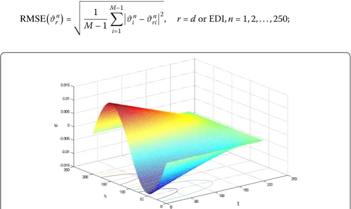
we only need to choose the POD basisΨ = [ϕ₁,ϕ₂, . . . ,ϕ₅] and compute the OCNFDE and OCNFDE/EDI solutionsϑ_din andϑ_EDIn _i(n= 1, 2, . . . , 250 andi= 1, 2, . . . , 250, i.e., 0 <t≤2.5 and 0≤x≤2.5) via the OCNFDE model (15) and the OCNFDE/EDI model (whoseG

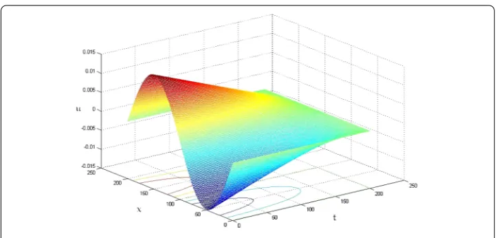
in (15) is replaced withGEDI), and depict them graphically in Figs.4and5, respectively. Figures4and5are almost the same.

To quantify the eﬃciency of the OCNFDE and OCNFDE/DEI methods, we compare the CPU time between the OCNFDE and OCNFDE/DEI methods, the root mean square errors (RMSE) between the CCNFD and OCNFDE solutions and between the CCNFD and OCNFDE/EDI solutions, and the correlation coeﬃcients (CC) between the OCNFDE and OCNFDE/EDI solutions. RMSE and CC are, respectively, obtained by means of the following formulas:

RMSEϑ_rn= 1

M– 1 M–1

i=1

ϑ_in–ϑ_rin2, r=dor EDI,n= 1, 2, . . . , 250;

(13)

Figure 5The OCNFDE/DEI solutions when 0≤t≤2.5 and 0≤x≤2.5

Table 2 Comparisons of CC, RMSE, and CPU time of the OCNFDE and OCNFDE/EDI solutions

n CC(n)×10–4 _{OCNFDE scheme} _{OCNFDE/EDI scheme}

RMSE CPU time RMSE CPU time

n= 150 1.6214 0.00032 2.88 seconds 0.00046 1.68 seconds

CC(n) =

250

i=1(ϑdin–ϑ¯din)(ϑEDIn i–ϑ¯EDIn i) 250

i=1(ϑdin–ϑ¯din)2 250

i=1(ϑEDIin –ϑ¯EDIn i)2

, n= 1, 2, . . . , 250,

whereϑ¯_rjn(r=dor EDI) are the expected values ofϑ_rjn, respectively. Table2shows that the CPU time between the OCNFDE and OCNFDE/DEI methods, RMSEs between the CCNFD and OCNFDE solutions and between the CCNFD and OCNFDE/EDI solutions, and CCs between the OCNFDE and OCNFDE/EDI solutions att= 1.5, 2.0, and 2.5, re-spectively.

Table2shows that the CPU time of the OCNFDE/EDI model is less than that of the OCNFDE one due to adopting EDI method, but it is reasonable that RMSEs of the OC-NFDE/EDI model is slightly larger than those of the OCNFDE model thanks to the non-linear termsGbeing approximated with EDI. It shows that the OCNFDE/EDI methd is better than the OCNFDE method.

6 Conclusions

(14)

so-lutions are proved by using the matrix analysis, so that the theoretical analysis and the numerical computations become more concise and convenient. In addition, as the OC-NFDE model for the FOPTSGEs (1)–(3) is ﬁrst established, it is an improvement of other existing reduced-order models mentioned in Sect.1.

Although we only have studied the order reduction of the CCNFD model for the FOPTS-GEs (1)–(3), because the CCNFD model can solve FOPTSFOPTS-GEs in a two- and three-dimensional unbounded domain (see, e.g., [3]), the OCNFDE model can easily and ef-fectively be applied to reduce the order for the FOPTSGEs (1)–(3) in two- and three-dimensional domains.

Acknowledgements

The authors are thankful to the editors and staﬀ of AIDE for their hard work in the publication of the paper.

Funding

This research was supported by the National Key Research and Development Project of China Grant 2017YFC1500301, the National Science Foundation of China grants 11671106 and 41704047, and the cultivation fund of the National Natural and Social Science Foundations in BTBU Grant LKJJ2016-22.

Availability of data and materials

The authors declare that all data and material in the paper are available and veritable.

Competing interests

The authors declare that they have no competing interests.

Authors’ contributions

Both authors contributed equally and signiﬁcantly in writing this article. Both authors wrote, read and approved the ﬁnal manuscript.

Author details

1_{School of Science, Beijing Technology and Business University, Beijing, China.}2_{School of Mathematics and Physics,}

North China Electric Power University, Beijing, China.

Publisher’s Note

Springer Nature remains neutral with regard to jurisdictional claims in published maps and institutional aﬃliations.

Received: 28 August 2018 Accepted: 19 December 2018

References

1. Dehghan, M., Manafian, J., Saadatmandi, A.: Solving nonlinear fractional partial differential equations using the homotopy analysis method. Numer. Methods Partial Differ. Equ.26(2), 448–479 (2010)

2. Kilbas, A.A., Srivastava, H.M., Trujillo, J.J.: Theory and Applications of Fractional Diﬀerential Equations. Elsevier, Amsterdam (2006)

3. Liu, F., Zhuang, P., Liu, Q.X.: Numerical Methods of Fractional Partial Diﬀerential Equations and Their Applications. Science Press, Beijing (2015) (in Chinese)

4. Cao, Y.H., Luo, Z.D.: A reduced-order extrapolating Crank–Nicolson ﬁnite diﬀerence scheme for the Riesz space fractional order equations with a nonlinear source function and delay. J. Nonlinear Sci. Appl.11, 672–682 (2018) 5. Elsaid, A., Hammad, D.: A reliable treatment of homotopy perturbation method for the sine-Gordon equation of

arbitrary (fractional) order. J. Fract. Calc. Appl.2(1), 1–8 (2012)

6. Yousef, A.M., Rida, S.Z., Ibrahim, H.R.: Approximate solution of fractional-order nonlinear sine-Gordon equation. Elixir Appl. Math.82, 32549–32553 (2015)

7. Macías-Díaz, J.E.: Numerical study of the process of nonlinear supratransmission in Riesz space-fractional sine-Gordon equations. Commun. Nonlinear Sci. Numer. Simul.46(1), 89–102 (2017)

8. Zhou, Y.J., Luo, Z.D.: A Crank–Nicolson finite difference scheme for the Riesz space fractional order parabolic type sine-Gordon equation. Adv. Differ. Equ.2018, 137, 1–7 (2018)

9. Sirovich, L.: Turbulence and the dynamics of coherent structures: parts I–III. Q. Appl. Math.45(3), 561–590 (1987) 10. Holmes, P., Lumley, J.L., Berkooz, G.: Turbulence, Coherent Structures, Dynamical Systems and Symmetry. Cambridge

University Press, Cambridge (1996)

11. Cazemier, W., Verstappen, R.W.C.P., Veldman, A.E.P.: Proper orthogonal decomposition and low-dimensional models for driven cavity ﬂows. Phys. Fluids10(7), 1685–1699 (1998)

12. Ly, H.V., Tran, H.T.: Proper orthogonal decomposition for ﬂow calculations and optimal control in a horizontal CVD reactor. Q. Appl. Math.60(4), 631–656 (1989)

13. Fukunaga, K.: Introduction to Statistical Recognition. Academic Press, New York (1990) 14. Jolliﬀe, I.T.: Principal Component Analysis. Springer, Berlin (2002)

15. Selten, F.M.: Baroclinic empirical orthogonal functions as basis functions in an atmospheric model. J. Atmos. Sci.

(15)

16. Kunisch, K., Volkwein, S.: Galerkin proper orthogonal decomposition methods for parabolic problems. Numer. Math.

90(1), 117–148 (2001)

17. Kunisch, K., Volkwein, S.: Galerkin proper orthogonal decomposition methods for a general equation in ﬂuid dynamics. SIAM J. Numer. Anal.40(2), 492–515 (2002)

18. Luo, Z.D., Chen, J., Navon, I.M., Yang, X.Z.: Mixed ﬁnite element formulation and error estimates based on proper orthogonal decomposition for the non-stationary Navier–Stokes equations. SIAM J. Numer. Anal.47(1), 1–19 (2008) 19. Luo, Z.D., Li, H., Zhou, Y.J., Xie, Z.H.: A reduced ﬁnite element formulation based on POD method for two-dimensional

solute transport problems. J. Math. Anal. Appl.385(1), 371–383 (2012)

20. Luo, Z.D., Yang, X.Z., Zhou, Y.J.: A reduced ﬁnite diﬀerence scheme based on singular value decomposition and proper orthogonal decomposition for Burgers equation. J. Comput. Appl. Math.229(1), 97–107 (2009)

21. Sun, P., Luo, Z.D., Zhou, Y.J.: Some reduced ﬁnite diﬀerence schemes based on a proper orthogonal decomposition technique for parabolic equations. Appl. Numer. Math.60(1–2), 154–164 (2010)

22. Luo, Z.D., Xie, Z.H., Shang, Y.Q., Chen, J.: A reduced ﬁnite volume element formulation and numerical simulations based on POD for parabolic problems. J. Comput. Appl. Math.235(8), 2098–2111 (2011)

23. Luo, Z.D., Li, H., Zhou, Y.J., Huang, X.M.: A reduced FVE formulation based on POD method and error analysis for two-dimensional viscoelastic problem. J. Math. Anal. Appl.385(1), 310–321 (2012)

24. Benner, P., Cohen, A., Ohlberger, M., Willcox, A.K.: Model Reduction and Approximation: Theory and Algorithm. Computational Science & Engineering. SIAM, Philadelphia (2017)

25. Hesthaven, J.S., Rozza, G., Stamm, B.: Certiﬁed Reduced Basis Methods for Parametrized Partial Diﬀerential Equations. Springer, Berlin (2016)

26. Quarteroni, A., Manzoni, A., Negri, F.: Reduced Basis Methods for Partial Diﬀerential Equations. Springer, Berlin (2016) 27. Dehghan, M., Abbaszadeh, M.: An upwind local radial basis functions-diﬀerential quadrature (RBF-DQ) method with proper orthogonal decomposition (POD) approach for solving compressible Euler equation. Eng. Anal. Bound. Elem.

92, 244–256 (2018)

28. Dehghan, M., Abbaszadeh, M.: A reduced proper orthogonal decomposition (POD) element free Galerkin (POD-EFG) method to simulate two-dimensional solute transport problems and error estimate. Appl. Numer. Math.126, 92–112 (2018)

29. Dehghan, M., Abbaszadeh, M.: A combination of proper orthogonal decomposition-discrete empirical interpolation method (POD-DEIM) and meshless local RBF-DQ approach for prevention of groundwater contamination. Comput. Math. Appl.75(4), 1390–1412 (2018)

30. Dehghan, M., Abbaszadeh, M.: The use of proper orthogonal decomposition (POD) meshless RBF-FD technique to simulate the shallow water equations. J. Comput. Phys.351, 478–510 (2017)

31. Luo, Z.D., Li, H., Sun, P., Gao, J.Q.: A reduced-order ﬁnite diﬀerence extrapolation algorithm based on POD technique for the non-stationary Navier–Stokes equations. Appl. Math. Model.37(7), 5464–5473 (2013)

32. Luo, Z.D., Gao, J.Q.: A POD-based reduced-order ﬁnite diﬀerence time-domain extrapolating scheme for the 2D Maxwell equations in a lossy medium. J. Math. Anal. Appl.444, 433–451 (2016)

33. Xia, H., Luo, Z.D.: An optimized ﬁnite diﬀerence iterative scheme based on POD technique for the 2D viscoelastic wave equation. Appl. Math. Mech.38(12), 1721–1732 (2017)

34. Xia, H., Luo, Z.D.: A POD-based optimized ﬁnite diﬀerence CN extrapolated implicit scheme for the 2D viscoelastic wave equation. Math. Methods Appl. Sci.40(15), 6880–6890 (2017)

35. Liu, S., Fu, Z.T., Liu, S.: Exact solutions to sine-Gordon-type equations. Phys. Lett. A351, 59–63 (2006)

36. Luo, Z.D., Chen, G.: Proper Orthogonal Decomposition Methods for Partial Diﬀerential Equations. Mathematics in Science and Engineering. Elsevier, Amsterdam (2018). https://www.elsevier.com/books/proper-orthogonal-decomposition-methods-for-partial-diﬀerential-equations/luo/978-0-12-816798-4

37. Chung, T.: Computational Fluid Dynamics. Cambridge University Press, Cambridge (2002)

38. Zhang, W.S.: Finite Diﬀerence Methods for Partial Diﬀerential Equations in Science Computation. Higher Education Press, Beijing (2006)

39. Chaturantabut, S., Sorensen, D.C.: Nonlinear model reduction via discrete empirical interpolation. SIAM J. Sci. Comput.