polarisation filter
Susan Loma Blakeney
University College London
A thesis submitted for the degree o f doctor of philosophy
ProQuest Number: U643809
All rights reserved
INFORMATION TO ALL USERS
The quality of this reproduction is dependent upon the quality of the copy submitted.
In the unlikely event that the author did not send a complete manuscript and there are missing pages, these will be noted. Also, if material had to be removed,
a note will indicate the deletion.
uest.
ProQuest U643809
Published by ProQuest LLC(2016). Copyright of the Dissertation is held by the Author.
All rights reserved.
This work is protected against unauthorized copying under Title 17, United States Code. Microform Edition © ProQuest LLC.
ProQuest LLC
789 East Eisenhower Parkway P.O. Box 1346
This thesis is concerned with researching novel applications for a commercially produced twisted nematic liquid crystal television display (TNLCTVD).
TNLCTVDs work by changing the polarisation of polarised light. The polarisation change is dependent upon the voltage applied to the display, and can be converted to an intensity change by viewing the display through a polariser (analyser). The amount of polarisation change is experimentally quantified in this thesis, and is used in two main applications. Firstly the LCTVD can be used as a Stokes polarimeter. The (unknown) polarisation of light passing through the display can be determined by recording the intensity transmitted by a fixed analyser when four separate voltages are applied to the LCTVD. These intensities are used to compute the Stokes vector of the incident light. This Stokes polarimeter has no moving parts, and is easily calibrated to cope with different environmental conditions, such as temperature, as well as different wavelengths of light. The polarimeter is shown to be accurate in determining the full state of polarisation, and can distinguish between partially linearly polarised and elliptically polarised light.
Table o f contents
TITLE
1
ABSTRACT
2
TABLE OF CONTENTS
3
LIST OF FIGURES
14
LIST OF TABLES
19
ACKNOWLEDGEMENTS
22
NOMENCLATURE AND ABBREVIATIONS
23
Part I - Introduction
Chapter 1 Introduction 26
1.1 Introduction to polarisation 26
1.2 Motivation for this work 27
1.3 Outline of the thesis 28
CHAPTER 2 POLARISATION
30
2.1 Introduction 30
2.1.1 Layout o f this chapter . 30
2.1.2 Polarised, unpolarised and partially polarised light 30
2.1.3 Types o f polarisation 31
2.1.4 Co-ordinate axes definition 31
2.2 Elliptical polarisation 32
2.3 Representations of polarisation 33
2.3.1 Jones vectors 34
2.3.2 Use o f Jones vectors 35
2.3.3 Calculation of ellipticity and azimuth angle from Jones vector 35
2.3.4 Calculation of Jones vector components from ellipticity and azimuth angle 35
2.3.5 The complex polarisation variable 36
2.3.6 The Poincaré sphere 38
2.3.7 Stokes vectors 38
2.3.8 Partial Polarisation 39
2.4 Producing and changing polarisation 39
2.4.1 Changing amplitude 40
2.4.2 Changing phase - birefringence 41
2.4.2.a Biréfringent materials 42
2.4.2.b Birefringence and liquid crystals 44
2.4.2.c The different use of birefringence and liquid crystals in this thesis 44
2.4.2.d Jones matrix of a biréfringent layer 45
2.5 Polarisation measurement: theory 46
2.5.1 Experimental quantification of polarisation 46
2.5.2 Intensity transmitted by a rotating analyser 46
2.6 Polarisation measurement: experiment 48
2.6.1 Imax/Imin method 48
2 .6 .2 lo, I45 and 1% m ethod 49
2.6.3 Linear regression of transmitted radiance sinusoid method 50
2.6.3.a Method used to determine accuracy of measurement 50
2.6.3.b Results 52
2.6.3.C Discussion: accuracy of azimuth angle and ellipticity measurements 53
2.6.3.C Conclusions 54
2.7 Intensity normalisation 54
2.8 Elliptically vs. partially linearly polarised light 55
CHAPTER 3 LIQUID CRYSTALS
56
3.1 Introduction: liquids, crystals and liquid crystals 56
3.2 Nematic liquid crystals 57
3.3 Anisotropy of Liquid Crystals 58
3.3.1 Viscosity 58
3.3.2 Birefringence (Optical Anisotropy) 58
3.3.3 Changes in a LC with application of an electric field (dielectric anisotropy) 59
3.3.4 Energetic Anisotropy 60
3.4 Liquid Crystal Displays 61
3.4.1 Alignment layers 62
3.4.2 The twisted nematic liquid crystal display 63
3.4.3 Freedericksz Transition 64
3.4.4 Thickness of TNLCDs 65
3.4.5 Optical modelling of TNLCDs 67
3.4.6.a Direct addressing 67
3.4.6.b Multiplexing 68
3.4.6.c Active matrix operation 68
3.4.6.d Field and row inversion addressing 68
3.5 Com parison of TNLCD perform ance with th a t of a parallel aligned nem atic
device 69
3.5.1 Description and uses of parallel aligned LC spatial light modulator 70
3.5.2 When the transmitted intensity is independent of LC voltage 71
3.5.3 Orientation of PALC cell and analyser 71
3.5.4 Contrast performance of parallel aligned NLC cell compared with
TNLCTVD 73
Part II - Polarisation filter
CHAPTER 4 LITERATURE SURVEY AND APPLICATIONS FOR A
POLARISATION FILTER
75
4.1 Introduction 75
4.2 P olarim eter proposed in this thesis using a commercially produced
LCTVD, o r a single pixel TNLC cell 76
4.3 P artial polarim eters 77
4.3.1 Non liquid crystal polarimeters 77
4.3.1.a With rotating components 77
4.3.1.b Without rotating components 77
4.3.2 Liquid crystal polarimeters: Liquid crystal polarisation camera 77
4.4 Full polarim eters 79
4.4.1 Non liquid crystal based polarimeters 79
4.4.1.a With rotating elements 79
4.4.1.b Without rotating elements 80
4.4.2 Liquid crystal polarimeters 80
4.4.2.a With rotating elements 80
4.4.2.b Without rotating elements 81
4.4.3 Wavelength dependence 81
4.5 Benefits of the polarim eter proposed in this thesis 82
4.6. l.c Determining refractive index or conductivity 84
4.6.l.d Surface quality assessment 86
4.6.1.e Gaining surface orientation information 86
4.6.2 Image enhancement 87
4.6.2.a Reducing unwanted reflections and highlights 87
4.6.2.b Scene edge detection 88
4.6.2.C Enhancing underwater visibilty 88
4.6.2.d Medical uses 88
CHAPTER 5 EXPERIMENTAL WORK ON THE POLARISATION FILTER
90
5.1 Introduction and aims 90
5.2 Design of experiment 90
5.2.1 Single pass 90
5.2.2 Double pass 91
5.3 Equipment used 91
5.3.1 Laser 91
5.3.2 NO filter 92
5.3.3 Quarter wave plate 92
5.3.4 Polariser 92
5.3.5 LCTVD 93
5.3.5.a Thickness 93
5.3.5.b Pixel pitch 93
5.3.5.C Brushing direction 94
5.3.5.d Driving signal 96
5.3.5.e Calibration fo contrast and brightness 96
5.3.5.f Stability of reading over time 97
5.3.6 Detector 97
5.4 Method 98
5.5 Results 98
5.6 Errors between model and experimental results 100
5.6.1 Experimental error 100
5.6.1.a Detector noise and unpolarised light 100
5.6. 1.b Azimuth angle variation 102
5.6.2 Temperature fluctuations 103
5.6.3 Diffraction pattern 103
5.6.4 Reflection 104
5.6.5 Driving signal 105
5.6.5.a Connection of oscilloscope 105
5.6.5.b Oscilloscope plots 105
5.6.5.C Discussion of oscilloscope traces 109
5.6.6 Interference and thickness variations of LC layer 110
5.6.6.a Spatial fluctuation of ellipticity measurements 110
5.6.6.b Thickness variation of LC layer 113
5.6.6.C The effect of interference, thickness variations, and driving signal 114
5.6.6.d Coherent and incoherent light 115
5.7 Optimisation 115
5.7.1 The problem 115
5.7.2 SVD to find least squares fit 117
5.7.3 Results of experimentally based Jones matrix model compared with the
theoretical model 118
5.7.4 Discussion 120
CHAPTER 6 ALGORITHM TO DETERMINE UNKNOWN INPUT
POLARISATION
122
6.1 Introduction & aims 122
6.2 Jones calculus method 123
6.2.1 Theory 123
6.2.2 Results 124
6.3 Stokes vector method 125
6.3.1 Theory 125
6.3.2 Calibration of LCTVD 126
6.3.3 Calculation o f unknown input Stokes vector 125
6.3.4 Results 126
6.3.4.a Using LCTVD 126
6.3.4.b Accuracy of measurement of input polarisation using LCTVD polarimeter 128
6.3.4.C Effect of errors 130
6.3.4.d Repeatability 131
6.3.4.e. Using single pixel LC cell 132
6.4.2.a Polyimide layer 136
6.4.2.b ITO thin film 136
6.4.2.C LC cell as reflecting cavity 137
6.4.2.d Electric field effects/variation in LC cell thickness 138
6.5 Discussion 140
6.5.1 Advantages of the LCTVD polarimeter 140
6.5.2 Polychromatic sources 141
6.5.2.a The problem 141
6.5.2.b How this affects the LCTVD polarimeter 141
6.5.2.C How other researchers have approached this problem 144
6.5.3 Oblique transmission 146
6.5.3.a Off axis reflection 146
6.5.3.b Off axis behaviour of LCD 147
6.6 Non-polarimeter applications 150
6.6.1 Reducing reflected highlights 150
6.6.2 Security mark reader 150
6.6.3 Polarisation encoding 150
Part III Security mark reader
CHAPTER 7 SECURITY DEVICE: INTRODUCTION AND LITERATURE
SURVEY
152
7.1 Introduction 152
7.1.1 Proposal for a polarisation varying security mark and automatic reader 153
7.1.2 Manufacturing methods 154
7.1.2.a Changing thickness 155
7.1.2.b Changing orientation 155
7.1.3 Verification 156
7.2 Requirements for a security mark 156
7.2.1 Difficult to replicate without authorisation 156
7.2.2 Cost effective 158
7.2.4 Easy to duplicate by an authorised party 159
7.3 Liquid Crystal security m ark reader; the concept 159
7.3.1 Original concept 159
7.3.2 Flaws in original concept 160
7.3.3 Improved concept 162
7.4 Relevant patents published 163
7.4.1 Security marks: 163
7.4.2 Reading systems 165
7.5 Phase masks 166
7.5.1 Advantages 167
7.5.2 Disadvantages and comparison 167
CHAPTER 8 SECURITY DEVICE
169
8.1 Introduction 169
8.2 Experim ental set-up used to measure and verify the security m arks 170
8.2.1 Overview 170
8.2.2 Light source 171
8.2.3 Liquid crystal display 172
8.2.4 Detection system 173
8.2.4.a Advantages and disadvantages o f CCD system over photodiode 173
8.2.4.b Settings used on CCD system/frame grabber and linearity of the system 173
8.3 Reading technique 174
8.3.1 Method 174
8.3.2 Registration of slides 175
8.3.3 Limitations of detector 175
8.3.4 Error calculation 176
8.3.5 Comparison points 177
8.4 Hull security marks 178
8.4.1 Manufacture and characteristics 178
8.4.2 AOI selection used to verify Hull slides 179
8.4.3 Experimental details 179
8.4.4 Results for Hull slides 180
8.4.4.a Using LCTVD 181
8.4.4.b Using single LC cell 183
8.5 Photographic quality security m arks from Rolic Research Ltd. 185
8.5.4 Experimental details 190
8.5.5 Results for Rolic photographic slides 191
8.5.6 Effect of polariser rotation 193
8.5.7 Effect of slide rotation 195
8.5.8 Effect of image rotation 197
8.5.9 Effect of image translation 198
8.6 Reproducibility of polarisation change caused by LC test cell over time 200
8.7 Discussion 201
8.7.1 Accuracy 201
8.7.2 Twisted nematic vs. parallel aligned nematic 202
8.7.3 Environmental changes 202
8.7.4 Wavelength 202
8.7.5 Density of information 203
8.7.6 Switching time 203
CHAPTER 9 DISCUSSION OF LC SECURITY MARK READER
204
9.1 Introduction 204
9.2 Statistical analysis of results from security mark reader 204
9.2.1 The problem and statistical solution 205
9.2.2 Customisation of cut-off point 206
9.3 Curve fitting: results 207
9.3.1 True slides 208
9.3.2 False slides 210
9.3.3 Summary 211
9.4 Distinguishing between true and false slides 211
9.5 Discussion 212
9.5.1 Sensitivity of reader 212
9.5.2 Customisation 213
9.5.3 Temperature changes 213
9.6 Summary 214
CHAPTER 10 CONCLUSIONS AND SUGGESTIONS FOR FUTURE
WORK
215
10.2 Comparison of TNLCD performance with that of a parallel aligned nematic
device 215
10.3 LC polarimeter 216
10.4 Security mark reader 217
10.5 Future work 218
10.5.1 Polarimeter 218
10.5.1.a Reflections 218
10.5.1.b Polychromatic sources 218
10.5.1.c Oblique incidence 219
10.5.1.d Machine vision applications 219
10.5.2 Security mark reader 219
10.6 Summary 220
Appendices
APPENDIX 2A SIGN CONVENTION AND SENSE OF ROTATION
221
2A.1 Definition of phase with respect to sense of rotation of light 221
APPENDIX 2B CALCULATION OF JONES VECTOR COMPONENTS
FROM ELLIPTICITY AND AZIMUTH ANGLE
224
APPENDIX 2C THE RELATIONSHIP OF THE STOKES PARAMETERS
TO THE CARTESIAN CO-ORDINATE SYSTEM AND POINCARÉ
SPHERE
226
APPENDIX 2D CHANGE OF POLARISATION ON REFLECTION FROM
A DIELECTRIC: THE FRESNEL COEFFICIENTS
228
APPENDIX 2E EFFECT OF BIREFRINGENT LAYER USING HUYGEN'S
WAVELET THEORY AND REFRACTIVE INDEX INDICATRIX
230
2E.1 Crystal plate cut with principal plane parallel to incident face of the
crystal 230
DIFFERING ANALYSER POSITIONS
232
2F.1 No liquid crystal present in optical system 232
2F.1.1 Input polarisation-30° 232
2F.2 Liquid crystal test cell present in optical system 234
2F.2.1 Voltage 0.784V (displayed voltage 1.99V) 234
2F.2.1.a Input polarisation 0 deg 234
2F.2.1.b Input polarisation-30° 235
2F.2.1.C Input polarisation-45° 236
2F.2.2 LC voltage 1.8478V (displayed voltage 4.1V) 237
2F.2.2.a Input polarisation-30° 237
2F.2.3 LC voltage 3.8649 (displayed voltage 8.1V) 238
2F.2.3.a Input polarisation-30° 238
APPENDIX 3A MULTIPLEXING OF LIQUID CRYSTAL DISPLAYS
239
3A.1 Multiplexing 239
3A.2 Active matrix operation 240
3A.2.I The benefits of active matrix addressing 240
3A.2.2 Field and row inversion addressing 241
APPENDIX 4A APPLICATIONS FOR POLARISATION MEASUREMENT
243
4A.1 Determining conductivity of a reflecting surface 243
4A.1.2 Intensity based method 243
4A. 1.2 Phase based method 243
4A.2 Highlight removal 245
4A.3 Medical uses 245
APPENDIX 5A CALIBRATION OF GREY LEVEL TO VOLTAGE
APPLIED TO LCTVD
247
APPENDIX 5B THE USE OF SINGULAR VALUE DECOMPOSITION IN
FINDING THE LEAST SQUARES SOLUTION
248
5B.1 Singular value decomposition method 248
5B.2 SVD and the least squares solution 250
APPENDIX 8A ORIENTATION OF EACH AREA OF EACH HULL SLIDE
RELATIVE TO POLYMERISING LASER
254
APPENDIX 8B CALCULATION OF PARAMETERS OF BIREFRINGENT
ROLIC SLIDES AREAS A AND B
255
APPENDIX 8C IMAGE PRO PLUS MACROS USED TO ANALYSE
SECURITY SLIDE IMAGES
258
8C.1 Macro used for Hull slides (dividing each slide into 9 areas) 258
8C.2 Macro used for Rolic photographic slides 261
APPENDIX 8D ADDITIONAL ERROR SCORES FOR ROLIC SECURITY
MARKS
263
8D.1 Error scores for Rolic slides 20 and 24 when polariser rotated 10 & 20
deg. 263
8D.2 Error scores for Rolic slide 24 when slide is rotated 264
Published papers
Use of a commercially produced liquid crystal display as a polarisation filter 265
Use of a commercially produced liquid crystal television as a security mark reader 278
Figure 2-1 Co-ordinate axes defined in this work... 32
Figure 2-2 Ellipse oriented at an angle alpha to the co-ordinate axes...33
Figure 2-3 - The circular complex polarisation variable...37
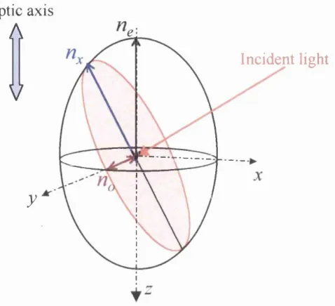
Figure 2-4 Index ellipsoid for a uniaxial (liquid) crystal... 43
Figure 2-5 Principal plane parallel to incident face of biréfringent crystal... 43
Figure 2-6 Ellipse of polarisation at an angle a to the co-ordinate axis... 47
Figure 2-7 The transmitted radiance sinusoid...47
Figure 2-8 Polariser calibration; input 0°... 52
Figure 3-1 Diagrammatic representation of nematic liquid crystal molecules, showing the director...57
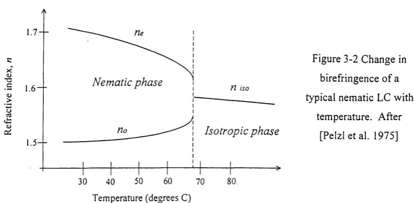
Figure 3-2 Change in birefringence of a typical nematic LC with temperature... 59
Figure 3-3 Change in Dielectric Constant of the Nematic Phase of 4-aminobenzonitrile with temperature... 60
Figure 3-4 Principle deformations in liquid crystals... 61
Figure 3-5 Twisted nematic liquid crystal cell: no voltage applied... 63
Figure 3-6 Twisted nematic liquid crystal cell: voltage applied... 63
Figure 3-7 To show Freedericksz transition for a parallel aligned LC cell with no pretilt. Angle o f director at midpoint as a function o f electric field... 64
Figure 3-8 Calculated transmission of a twisted nematic structure as a function o f cell thickness...66
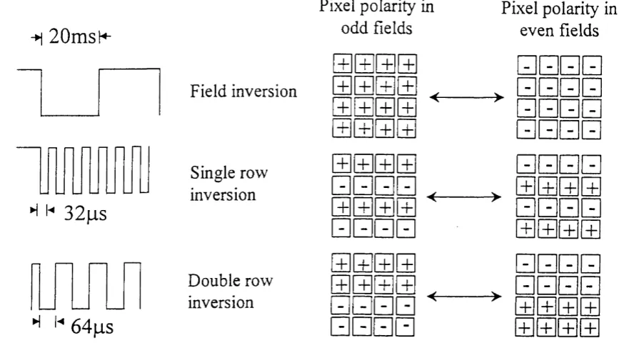
Figure 3-9 Methods of a.c. addressing of LCTVDs. Addressing rate 50Hz, 625 rows... 69
Figure 3-10 Arrangement of LC director in a parallel aligned nematic LC cell. No voltage applied... 70
Figure 3-11 Parallel aligned nematic LC cell. Voltage applied... 70
Figure 3-12 Director tilt/intensity curve for PALC cell... 73
Figure 3-13 Voltage/intensity curves for LCTVD... 74
Figure 4-1 Layout of LCTVD polarimeter... 76
Figure 4-2 Liquid crystal polarisation camera... 78
Figure 4-3 Fresnel ratio versus specular angle o f incidence...86
Figure 5-1 Layout of experiment in single pass...91
Figure 5-2 Layout of pixels on LCTVD... 93
Figure 5-4 Intensity transmitted through unswitched LCTVD through parallel polarisera 95 Figure 5-5 Change in calculated transmission obtained through parallel polarisers through
unswitched LCTVD... 95
Figure 5-6 Variation of intensity transmitted through crossed polarisers vs. GL...97
Figure 5-7 Single pass results for LCTVD... 99
Figure 5-8 Comparison of theoretical and experimental ellipticity measured using linear regression. 9 experimental GLs used... 101
Figure 5-9 Fluctuation of resultant polarisation for input polarisations of -15° and +45° passing through LCTVD. GLs 255, 140 and 0... 102
Figure 5-10 Variation of An with temperature for LCTVD...103
Figure 5-11 Connection of oscilloscope to photodetector... 105
Figure 5-12 Variation of photodetector response during one frame tim e...106
Figure 5-13 Background noise recorded when the light source was covered... 107
Figure 5-14 Changes in output ellipticity values with specific values of intensity taken from the frame time. Input-15°... 108
Figure 5-15 Changes in output ellipticity values with specific values of intensity taken from the frame time. Input -75°... 109
Figure 5-16 Voltage intensity curve of LCTVD. Different analyser positions. Theoretical model...1 10 Figure 5-17 Translation of LCTVD horizontally; maximum and minimum intensities measured with vernier position...111
Figure 5-18 Translation of LCTVD horizontally: resultant ellipticities from intensities shown in Figure 5-17... 111
Figure 5-19 Variation in values for a for light emerging from LCTVD (unswitched). Input polarisation +45°. Various theoretical models... 113
Figure 5-20 Variation in values for e for light emerging from LCTVD (unswitched). Input polarisation +45°. Various theoretical models... 114
Figure 5-21 Experimental polarisation change produced by LCTVD compared with that predicted by SVD and theoretical Jones matrix models. Input polarisation circular 119 Figure 5-22 An expansion of Figure 5-21 to show experimental errors...120
Figure 6-1 Use o f LCTVD as Stokes polarimeter. Polarimeter-measured and actual input polarisations... 128
Figure 6-4 Variation in total intensity transmitted by single pixel LC cell... 133
Figure 6-5 Construction of LC cell, to show reflecting layers... 135
Figure 6-6 Variation of reflectance (from ITO/LC interface) with absorption coefficient of ITO (normal incidence)...136
Figure 6-7 Plane parallel plate: illustrating the formation of fringes at infinity... 138
Figure 6-8 Variation of reflected intensity (between ITO and LC layer) with refractive index of LC layer (0° twist)... 139
Figure 6-9 Variation of reflected intensity (between ITO and LC layer) with director orientation (0° twist)...139
Figure 6-10 Effect of changing LC thickness on reflected intensity (between ITO and LC layer) for rio and n^. Parallel aligned cell... 140
Figure 6-11 Change in refractive index of LCTVD with wavelength... 143
Figure 6-12 Variation of results obtained (using theoretical model including dispersion) for different wavelengths (400-700nm) using Mueller matrix model for SSOnm...144
Figure 6-13 Change in intensity transmitted by analyser with wavelength for fully switched and unswitched states of LCTVD... 146
Figure 6-14 Effect of oblique viewing angles: simplified structure of TNLC cell showing orientation of mid-plane director for mid-high voltage... 148
Figure 6-15 Calculated variation in transmission, T, for a normally white TNLC cell with horizontal viewing angle for various applied voltages...149
Figure 6-16 Calculated variation in transmission, T, for a normally white TNLC cell with vertical viewing angle for various applied voltages... 149
Figure 6-17 An optical system for converting incident polarised light to any state of polarisation...151
Figure 7-1 Security mark reader in transmission mode... 154
Figure 7-2 Security mark reader in reflection m ode...154
Figure 7-3 Spatial variation of birefringence...155
Figure 7-4 Variation in azimuth angle and ellipticity vs. biréfringent film thickness...158
Figure 7-5 Proposed use of LCD to verify biréfringent security m ark... 160
Figure 7-6 Values of ellipticity and y needed to transmit a constant intensity... 161
Figure 8-1 Experimental arrangement used for measuring and verifying the security mark.... 171
Figure 8-2 LED stability with tim e... 172
Figure 8-4 Image of slide 3 through single LC cell. LC cell off... 179
Figure 8-5 Diagrammatic illustration of areas of slide 3... 179
Figure 8-6 Histogram of error scores. True slides only. C>0. LCTVD as reader... 181
Figure 8-7 Histogram of error scores. False slides only. O O . LCTVD as reader... 181
Figure 8-8 Histogram of error scores. True slides only. C>10. LCTVD as reader...182
Figure 8-9 Histogram of error scores. False slides only. C>10. LCTVD as reader... 182
Figure 8-10 Histogram of error scores. True slides only. C>0. LC cell used as reader 183 Figure 8-11 Histogram of error scores. False slides only. C>0. LC cell used as reader 183 Figure 8-12 Histogram of error scores. True slides only. C>10. LC cell as reader... 184
Figure 8-13 Histogram of error scores. False slides only. C>10. LC cell as reader... 184
Figure 8-14 Image of slide from Rolic Ltd... 186
Figure 8-15 Experimental layout for measuring birefringence...of Rolic slides... 186
Figure 8-16 Change in ellipticity and azimuth angle of polarisation with And and Û of biréfringent layer. Input polarisation 0°...187
Figure 8-17 Change in ellipticity and azimuth angle of polarisation with And and <9 of biréfringent layer. Input polarisation 60°... 187
Figure 8-18 Bubble plot of optimum values o f And and 6 for Rolic slides areas A and B. Four different input polarisations... 188
Figure 8-19 Slide 22, LC cell o ff...190
Figure 8-20 Slide 22, LC cell 1.85V...190
Figure 8-21 Slide 22, LC cell 2.56V...190
Figure 8-22 Slide 22, LC cell 3.86V...190
Figure 8-23 Image o f slide 22, LC cell 1.85V. Rotation +10°... 191
Figure 8-24 Image o f slide 22, LC cell 1.85V. Rotation -10°... 191
Figure 8-25 True Rolic slides. C^O... 191
Figure 8-26 False Rolic slides. C>0... 192
Figure 8-27 True Rolic slides. C^lOO... 192
Figure 8-28 False Rolic slides. C^lOO...193
Figure 8-29 Rolic slide 22 only. Comparison of error score with polariser at 0° (‘true’), 10° and 20°. All points considered (C >0)... 194
Figure 8-30 Rolic slide 22 only. Comparison of error score with polariser at 0° (‘true’), 10° and 20°. C >100... 195
Figure 8-31 Rolic slide 22, effect of slide rotation on error score... 196
voltages...200
Figure 9-1 Demonstration of false negative and false positive results around intersection of error score curves... 206
Figure 9-2 Same graphs as in Figure 9-1, but with area under false slide curve increased by 5 ... 207
Figure 9-3 Best curve fits obtained for true Rolic slides histogram...209
Figure 9-4 Best curve fits obtained for false Rolic slides histogram... 210
Figure 9-5 Best curve fits to true and false Rolic slides. Graph enlarged to show intersection.... 211 Figure 2A-1 Relative phase of-r and y components of electric field... 221
Figure 2A-2 Sign convention for phase difference when sense of rotation is right handed (looking away from source)...222
Figure 2A-3 Vibration of electric vector...222
Figure 2A-4 Same wave as in Figure 2A-3, at some later point in time... 223
Figure 2E-1 Ordinary and extraordinary wavefronts and rays in a uniaxial crystal when a plane wave is incident normally to the surface and to the optic axis...230
Figure 2E-2 An incident plane wave polarised perpendicular to the principal section...231
Figure 2E-3 An incident plane wave polarised parallel to the principal section... 231
Figure 2F- 1 Experimental intensity measured through analyser vs. cos^ y. Input polarisation -30° (linear)...232
Figure 2F- 2 Experimental vs. theoretical intensity. Various analyser positions. Input 0°, LC cell voltage 0.784V... 234
Figure 2F- 3 Experimental vs. theoretical intensity. Various analyser positions. Input -30°, LC cell voltage 0.784V ...235
Figure 2F-4 Results using LC cell at 0.7834V voltage. Input polarisation -45°... 236
Figure 2F-5 Results using LC test cell at 1.8478V voltage. Input polarisation -30°... 237
Figure 2F- 6 Results using LC cell at 3.8649V. Input polarisation -30°... 238
Figure 3A-1 Multiplexing of LCD pixels... 239
Figure 3A-2 Change in brightness of LC display with increasing voltage... 240
Figure 3A-3 Methods of a.c. addressing of LCTVDs. Addressing rate 50Hz, 625 rows...242
Figure 5A-2 Relationship between GL and voltage for LCTVD... 247
Table 2-1 Changes in values for a and e with varying number of intensity readings taken. Linearly polarised input, no LC present...53
Table 5-1 Variation in values of a and e for ‘circularly’ polarised light falling on first polariser, depending on how many analyser positions were used to measure intensity (using linear regression method described in s.2.6.3)...93
Table 5-2 Variation in ellipticity values obtained on translating the LCTVD by 14mm horizontally. Input polarisation -15°... 112
Table 6-1 Values for a and e for input polarisation of +30° (linear) if theoretical intensities are corrupted by error... 124 Table 6-2 Effect of error on LCTVD Stokes polarimeter. Theoretical intensities corrupted by
10 or 2%... 131 Table 6-3 Mean and standard deviation values for a, e and P for the polarisations shown in Figure 6-3. Repeat readings for input linear polarisation of 60°...131
Table 8-1 Mean and standard deviation values for the error score histogram shown in Figure 8-29. (O O ) ... 194 Table 8-2 Mean and standard deviation values for the error score histogram shown in Figure
8-30. (C > 10 0)... 195 Table 8-3 Mean and standard deviation values.for the error scores shown in Figure 8-31...196 Table 8-4 Mean and standard deviation values.for the error scores shown in Figure 8-32...198 Table 8-5 Mean and standard deviation values.for the error scores shown in Figure 8-33...199
Table 9-1 Standard errors and correlation coefficients for curves fitted to true slide data...209 Table 9-2 Standard errors and correlation coefficients for curves fitted to false slide data. 211 Table 9-3 Effect o f the different curve fits shown in Figure 9-5 on misclassification of slides....
212
Table 2F-5 Changes in values for a and e with varying number of intensity readings taken. Input polarisation-30°. Test cell voltage 1.8478V... 237 Table 2F-6 Changes in values for a and e with varying number of intensity readings taken.
Input polarisation -30°. LC cell voltage 3.8649V... 238
This thesis would not have been possible without the help of many people:
Firstly, I would like to thank my supervisors, Sally Day and Neil Stewart, for their great help and encouragement. I must also thank my colleagues at Sira, particularly Jason Dale and Tom Benson, and the members of the optical devices research group at UCL, particularly Mark Gardner, Robin Kilpatrick and Lawrence Commander, for their suggestions and support. Life over the past few years would have been far more boring without all of them. David Selviah at UCL also deserves thanks for stepping into Sally’s shoes when she was on maternity leave. Two other people at Sira also deserve a mention: MarkHodgetts was always on hand for mathematical discussions, and John Gilby was a breath of fresh air and innovation when I needed it. Alistair Greig at UCL is the culprit who suggested I embark upon this work and as recompense for that suggestion has been kind enough to give me his comments on this thesis.
Several companies were very generous with their assistance: Philips Research Laboratories in Redhill very kindly supplied the LCTVD and single pixel LC cell which were used throughout this work. Andy Pearson from Philips (always on the end of an e-mail !) was extremely patient and helpful with his technical knowledge, and Anette Hultaker o f Uppsala University very kindly sent me a copy of her licentiate thesis on ITO films. The biréfringent film used for the prototype security marks, and the LC polymer used to make the ‘Hull’ security marks was kindly supplied by Merck, and both Richard Harding and Mark Verrall from Merck deserve kind thanks for their help. Rolic Research provided the photographic quality biréfringent security marks that were invaluable when testing the security mark reader, and GSI kindly provided the superbright LED. Perry Jackson at Hull University was an angel for helping me make the ‘Hull’ security marks.
This work was undertaken as part of the Sira/UCL postgraduate training partnership which is a joint initiative between the DTI and the EPSRC and funded by the EPSRC, DTI and Sira Ltd (thank you very much).
N o m e n c la tu re
Nomenclature and abbreviations used
a
e
X
Cù a
b (=E y)
a ’ b ’ C d e E exp GL
Im a x
^min le k LC LC(TV)D n Ue rio Ux An And PA QWP
Phase difference {</)=<ffx-(py)
Azimuth angle of polarisation ellipse Angle of analyser (with respect to % axis) Wavelength
Angular frequency (=2 7^, where / i s the frequency)
Amplitude of x vibration Amplitude of y vibration
Half length of major axis of polarisation ellipse Half length of minor axis of polarisation ellipse
Number of comparison points (used in security mark verification) Thickness of optical layer
Ellipticity of polarisation ellipse {=a’'/b "')
Electric vector, or error score used in security mark verification, depending on context
Exponential
Grey level (applied to LCTVD or measured from the image of the security mark)
Maximum intensity measured on rotation of analyser Minimum intensity measured on rotation of analyser Intensity measured through analyser at angle 6 Wave constant (=2n/X)
Liquid crystal
Liquid crystal (television) display Refractive index
Extraordinary refractive index Ordinary refractive index
Refractive index as determined by index indicatrix Birefringence {=nx-n„; or ne-nj
Retardance (may be multiplied by 27t) Parallel aligned (nematic)
Quarter wave plate
SLM t
TN TRS z
J , iJ J ^ + i J
So'
^3.
Spatial light modulator Time
Twisted nematic (liquid crystal) Transmitted radiance sinusoid
Distance travelled by wave (along z axis)
Jones vector (J/, Jj, J3 and J4 are real numbers)
‘Light is characterized by its intensity, wavelength, and polarization.’
Chapter 1
ntroduction
1.1
Introduction to polarisation
Despite the interference experiments carried out by Thomas Young (1773-1829), it was not until the experiments ofFresnel and Arago in 1818 that it was discovered that light had no longitudinal components, but consisted only of two transverse vibrations [Collett, 1993, p.22]. These vibrations are perpendicular to each other. For convenience, the axis system can be chosen so that these vibrations are along thex and y axes, and the light is propagating in the z direction. The combination of these transverse components of light leads to the polarisation ellipse, but it was not until Sir George Stokes published his papers in 1852, that an adequate mathematical description could be given to describe the various states of polarisation that can occur. The mathematical description of polarised light is discussed in Chapter 2. The Stokes vectors are still used today, and have an advantage of being experimentally defined because they are constructed around the measurements of intensity, not amplitudes. They will be used in this thesis, particularly in Chapter 6.
Chapter 1 Introduction
reflecting material and its orientation. Use of polarisation for image analysis will be discussed in Chapter 4. Information can also be encoded as a polarisation pattern. This pattern is invisible unless special polarisation decoding apparatus is used. This will be discussed in Chapters 7-9.
The author’s enthusiasm for the subject of this thesis was inspired by the fact that the polarisation of light is so fundamental a property, and is affected by so many things (optical activity, scattering, reflection etc), but humans are completely insensitive to it'. In addition to the wavelength and intensity of light, polarisation can carry additional information [Wolff, 1997] to which humans are not privy without special equipment (at the least a polarising sheet). This thesis aims to make that information acquirable using a commercially produced liquid crystal display.
1.2
Motivation for this work
Liquid crystal displays (LCDs) are commercially available for many applications. These include simple passive matrix addressed displays, such as those used in digital watches and calculators, and the more complex actively addressed displays which are used in displays for computer and television screens. The mass market for LCDs results in them being produced at relatively low cost, and this has led to researchers looking for alternative uses of these displays. The high cost of commercial spatial light modulators (around £9000 [Hamamatsu, 2000]- see Chapter 10) has encouraged researchers to use modified liquid crystal television displays (LCTVDs) for spatial light modulation since approximately 1985 [Aiken & Bates, 2000; Wolff, 1997]. A LCD works by changing the polarisation of (polarised) light passing through it, and this thesis looks at using a LCTVD as a polarisation filter. This varies from the use of a LCTVD as a spatial light modulator because polarisation is changed by the phase difference between the orthogonal components o f the light mentioned above. Spatial light modulators are concerned with the phase of one area of the incident wavefront compared with another, regardless of its polarisation state.
Two main applications are considered:
1) Using the LCTVD as a complete polarimeter. An algorithm is presented which enables unknown input polarisation to be determined by recording the intensity o f light transmitted through the LCTVD and a fixed analyser. The state o f polarisation can be
calculated from intensity measurements taken at four voltages of the LCTVD", This avoids the need for any mechanically rotating parts.
2) The LCTVD can also be used as a security mark reader for authenticating security marks which emit a known pattern of polarisation. Polarisation varying security marks are difficult to counterfeit, partly because they cannot be reproduced photographically. The large number of patents that have been published detailing the production of such marks indicates the usefulness of a polarisation varying security mark. However, there have been no such publications that detail an automatic method of authenticating these marks. This thesis describes how this can be done using a LCTVD or a single LC cell. This is discussed in Chapters 7-9.
When a LCTVD is used as a display, the polarisation change is converted to an intensity change by viewing the display through a (second) linear polariser. However, this conversion of polarisation change to intensity change means that the phase information (which partly determines the state of polarisation) is lost. This can be likened to converting a three dimensional image to a two-dimensional photograph. This work looks at the use of a commercially produced liquid crystal television display (LCTVD) in the polarisation, rather than the intensity, domain. Using a commercially available device has the advantage that the device is easily reproduced, and done so at lower cost than if it were custom made.
1.3
Outline o f the thesis
The thesis is arranged in three main sections:
Part I (Chapters 1-3) outlines the background behind liquid crystals and polarisation.
Nematic liquid crystal displays only work with polarised light. The theory of polarisation,
including the mathematical treatment of birefringence and how polarised light can be produced
and manipulated is therefore discussed first in Chapter 2. What a liquid crystal is, why liquid
crystals are so special, and how liquid crystal displays work is covered in Chapter 3.
Part II (Chapters 4-6) discusses the background theory, experimental work,
optimisation and algorithm behind using the LCTVD as a polarisation filter to determine
unknown polarisation. If light of unknovm (full or partial) polarisation is passed through the
LCTVD and a fixed analyser, the LCTVD can be used as a ‘Stokes-meter’. This means that by
simply applying four voltages to the LCTVD and measuring the intensity of the light
transmitted by the analyser, the polarisation of the incident light can be determined. This
enables the full polarisation state to be measured without any rotating components. A
Chapter 1 Introduction
comparison of a method that uses Jones calculus with that using Mueller calculus is discussed in Chapter 6.
Part III (Chapters 7-9) discuss the use of the LCTVD or a single LC cell (which is very similar in construction to the LCTVD, but only consists of one pixel) as part of a reader which can authenticate polarisation varying security marks. As a precaution against counterfeiting, it may be desirable to attach a mark to an article that indicates its authenticity. Such a mark could be made to emit a spatially varying pattern of polarisation when it is illuminated with polarised light. This pattern would be invisible to the unaided eye and difficult to counterfeit. Part III will detail the use of the LCTVD (or single LC cell) as part of an automatic verification system for these marks, the sensitivity of which could be customised to meet the needs of the user. The production of such marks, together with the advantages and disadvantages of such a system is discussed.
Chapter 2
olarisation
2.1
Introduction
2.1.1 Layout of this chapter
This chapter will begin by describing what polarised light is, and the different forms of polarisation that can occur. It will then (s.2.3) describe different methods (including Jones vectors and Stokes vectors) for mathematically representing these different polarisations. The methods o f producing polarised light will be discussed in s.2.4, together with how these methods can be represented mathematically, to interact with the representations of polarised light discussed in s.2.3. The measurement of polarisation will be covered in s.2.5 and s.2.6 and the merits o f different techniques will be discussed. Section 2.7 outlines how the intensity of the polarisation ellipse can be normalised, and s.2.8 deals with the distinction between partially linearly polarised and fully elliptically polarised light.
2.
1.2 Polarised, unpolarised and partially polarised light
Chapter 2 Polarisation
of the magnetic vector, which is always orthogonal to the electric vector, will not be explicitly mentioned in this thesis. Any references in this thesis to the field vector or its vibration should be taken as referring to the electric field vector.
If the polarisation state changes more rapidly than the speed of observation, the light is called partially polarised, or unpolarised depending on the time-averaged behaviour of the polarisation state [Yeh & Gu, 1999, p.34]. Unpolarised light occurs when the end point of the electric vector moves quite irregularly, and the light shows no preferential directional properties when resolved in different directions (at right angles to the direction of propagation). Partially polarised light is light that is neither completely polarised, nor completely unpolarised. This thesis is mainly concerned with light which is completely or almost completely polarised (i.e. the unpolarised component, if present, is very small compared to the polarised component) and this will be described in more detail. Partial polarisation will be discussed briefly in this chapter for completeness and because in some circumstances it can be confused with elliptically polarised light (see s. 2.3.8 and 2.8).
2.
1.3 Types of polarisation
The state of polarisation of light depends on the relative amplitudes of the transverse components of the electric field along thex and y co-ordinate axes, and the phase difference between them, (f>. The most general description of polarisation is elliptical polarisation, because the tip of the electric vector traces out an ellipse in time (or space). This will be described in s.2.2 below. Linear and circular polarisations are special forms o f elliptical polarisation. They occur when ^ is an exact multiple of tt, or an odd multiple o f n il respectively. For the light to be circularly polarised, as well as the phase difference being an odd multiple o f 7i/2, the amplitudes of the x and y components have to be equal.
Completely linearly polarised light can be extinguished by passing it through an ideal polariser whose transmission axis is perpendicular to the plane of vibration of the electric vector o f the incident light. This principle can be extended to cover all polarised light, by defining light as being fully polarised if a quarter wave plate (QWP) (see s. 2.4.2 below) followed by an ideal polariser can be used to extinguish the beam [Mansuripur, 2000].
2.1.4 Co-ordinate axes definition
-ve rotation +ve rotation
Figure 2-1 Co-ordinate axes defined in this work
Light propagates along the z direction
2.2
Elliptical polarisation
The two components of a light wave vibrating along the x and y axes can be represented as [Born & Wolf, 1999, p.25 et seq.]:
= a cos[cüt -A z-t-y) equation 2-1
E y = b cos{cot — Az — y j equation 2-2
Where a and b are the amplitudes of the x and y components respectively, k is the wave constant {=2 tc/X), cû is the angular frequency (=2tc/ where/ is the frequency in hertz),
and t is the time in seconds. If the absolute phase of thex component is defined as and that o f the y component is ^ then ^ is the phase difference between the orthogonal vibrations (defined so (f>=(f>x- (f>y). When sin <f> is negative, the x vibration leads the y, so the light is defined as right-handed (see Appendix 2A). This represents the tip of the electric vector tracing a clockwise rotation when the observer looks towards the source [Azzam & Bashara, 1979, p.39]. Adding these two vibrations leads to the equation of an ellipse oriented at an angle or to the co-ordinate axis [Bom & Wolf, 1999, p.25 et seq.] - equation 2-3. It can be seen that the sign of <f> does not alter this equation.
2 f E '\( E equation 2-3
y
- 2cos^ ’ a
y
= sin (f> \ o j
This is illustrated in Figure 2-2. a is defined so -180°< a <180° An azimuth angle o f +30° is equivalent to one of -150° '.
Chapter 2 Polarisation
Figure 2-2 Ellipse oriented at an angle alpha to the co-ordinate axes
The azimuth angle of the ellipse, a, is given by equation 2-4 [Bom & Wolf, 1999, p.28].
1
a - —tan-1
2ab cos(j) equation 2-4
The magnitudes of the major and minor axes of the ellipse can be calculated from the original amplitudes of the vibrations, and the phase difference between them (equation 2-5 and equation 2-6 [Collett 1993, p.28]).
.2 _ 2 „ O______ :_______A COS ÛT sin a 2 COS ûf sin a COS ^ sin ^
. 2
ab
(o')
, \ 22
sin 6% cos a 2 cos a sin or cos sin é : — + •
equation 2-5
equation 2-6
a"- b^ ab {b 'Ÿ
In this thesis, polarisation is defined using the azimuth angle of the ellipse, a, and its
ellipticity, e, defined so that ^ ~ ~ p2 - should be noted that this is the square o f the
reciprocal of the definition in some textbooks.
2,3
Representations o f polarisation
are more mathematically complex than Jones vectors because the Mueller calculus that is needed to transform one [4 x 1 ] Stokes vector into another involves [4 x 4] matrices, whereas the matrices needed to transform the [ 2 x 1 ] (complex) Jones vectors are only [2 x 2]. Additionally, because Stokes vectors do not include phase information, they do not describe coherent light. However, the Stokes representation can be used when the light is not completely polarised, and the intensity based definition means that it is possible to look at a Stokes vector and immediately have some knowledge about the state of polarisation (see s.2.3.7).
Jones calculus does not describe partially polarised light, or optical systems which depolarise. This disadvantage can be circumvented if partially polarised light is thought o f as a combination of completely polarised light and completely unpolarised light [Clarke & Grainger, 1971, p.31; Chen & Wolff, 1998). It is also not normally easy to tell the state of polarisation simply by looking at a Jones vector - calculations have to be performed on the vector before the exact state of polarisation is known. Jones calculus is covered in [Jones, 1941] and [Jones, 1942]. A complete discussion of the difference between Stokes and Jones vectors can be found in [Azzam & Bashara, 1979, pp. 13-65].
Many papers have covered the modelling of liquid crystal cells using Jones matrices (such as [Gooch & Tarry, 1975], [Raynes. & Tough, 1985], [Raynes, 1987]). A Jones matrix model o f the LCTVD, which has been developed by researchers at UCL, is used in this work [Kilpatrick et al., 1998]. Consequently Jones calculus is initially used in this thesis. However, Stokes vectors will also be used in Chapter 6, so this representation is also discussed in this chapter (section 2.3.7).
2.3.1 Jones vectors
Jones calculus represents a polarised beam of light by a column vector whose elements are the two components (£* and Ey) of the electric vector. The vectors express the amplitudes and phases o f the x and y components individually. It is understood that the physical displacements o f the E vector are given by the real parts of the two elements [Robson, 1974]. Using the notation in equation 2-1 and equation 2-2 the Jones vector describing the polarisation would be;
equation 2-7
be'*'
The amplitude and phase of the waves are preserved using the complex notation. If the exact phases of the constituent waves are not needed, the phase of the x component can be removed from the vector, by dividing both components by exp(/^v), to get:
Chapter 2 Polarisation
E = e'* a
be~‘*
The 2x1 complex Jones vector has four components: y , + iJ 2 ^3 + / J4
equation 2-8
. To normalise this vector,
the components can all be divided by + ^3" + ^4^ [Hecht, 1998, pp.366-368].
2.3.2 Use of Jones vectors
Jones vectors are a mathematical tool for analysing the effect of various (non depolarising) optical components on the passage of polarised light. To determine the polarisation represented by each vector, the amplitude and phase information needs to be re introduced to the oomplex vector, and from this ellipticity, azimuth angle and sense of rotation o f the polarisation ellipse can be calculated. The methods for converting a Jones vector (a, b, and to a and e, and back again are covered below:
2.3.3 Calculation of ellipticity and azimuth angle from Jones vector
The Jones vector Re(x) + Im(x) allows the phase of the x and y components to be
_Re(>^)-Flm(»
calculated directly from the Argand diagram of the individual phasors (equation 2-9).
(j>^ =tan-1 Im(%) Re(%)
equation 2-9
The amplitudes o f the components are calculated by taking the square root o f the phasor multiplied by its complex conjugate. The azimuth angle of the ellipse can now be calculated using equation 2-4. Similarly, the major and minor axes can be calculated using equation 2-5 and equation 2-6.
2.3.4 Calculation of Jones vector components from ellipticity and
azimuth angle
The mathematical procedures for calculating the Jones vector components are detailed in Appendix 2B. The ratio a^/b^ can be calculated using:
equation 2-10 a^ b'^ sin^ a + a'^ cos^ a
To calculate the phase difference, <j), equation 2-4 can be written:
2 —c o s^ tan 2 a = ^ ' + fnrr
equation 2-11
Therefore,
cos (j) = tan 2a
1
-a
equation 2-12
equation 2-12 contains the ratio a/b, which can only be calculated by taking the square root of equation 2-10. This results in a sign ambiguity. This can be resolved if equation 2B-9 is divided by equation 2B-8 (equations in Appendix 2B):
bcos(/>
= cos a sin a
equation 2-13
a
a'^ CQS^ a + b'^ sm^ a
If the sense of rotation of light is measured, the sign of cos (f) is known, equation 2-13 therefore enables the sign of a/h can be deduced. Changing the sign of both imaginary components in the Jones vector changes the sense of the light, whilst retaining the original ellipticity and azimuth angle.
It is a simple matter to calculate the Jones vector components from a, h and (j>, as the complex phasors are simply {a exp /^ 2 ) and {h exp The real part of thex component, A, is simply {a cos ^ 2 ) and the imaginary part, B, is (a sin ^2 ). The same can be done for the y phasor. Absolute phase does not affect polarisation, so, in most of the calculations in this
thesis the Jones vectors are arranged so that the phase of the x component is zero.
2.3.5
The complex polarisation variable
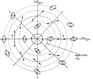
One method of representing the polarisation o f light, which will be used in this thesis, is that described by Azzam & Bashara [1979, pp.39-49; and 1972]. This is to use the complex polarisation variable, %with the basis states of polarisation as the R and L states. Instead of using the linear x and y orthogonal components, as described above, % represents the ratio of the circular complex Jones vectors (equation 2-14).
1^1
where (j>r and are the phases of the R and L orthogonal components. Then
Chapter 2 Polarisation
\Z \ =
E,
and arg (;r ) = # -(4
An advantage of this representation is that, when the Argand diagram is plotted, the state o f polarisation represented by points on the diagram can be seen easily. Linear polarisation states are represented by a concentric circle about the origin, with a radius of 1. The origin and infinity represent left and right circular polarisations respectively. Polarisations which are left handed all fall within the circle of linear polarisations, and those which are right handed all fall outside it (see Figure 2-3). Concentric circles represent loci of polarisations with equal ellipticities, and radial lines represent polarisations with equal azimuth angles.
Figure 2-3 - The circular complex polarisation variable (from Azzam & Bashara, 1979, p.42)
The familiar values of azimuth angle, a, and ellipticity, e can be found from manipulation o f the definition of the Jones vector with r and / as its basis states - i.e.
E expf^ equation 2-15
Ej expz^/
To calculate % from the known values of a and e we use the relationship:
The azimuth angle can be found directly from the plot, because a - - y a r g (2') [Azzam & Bashara, 1979, p.40], so
a = jta n ' Im (z ) Re(%)
equation 2-17
b' 1
Azzam and Bashara define the ellipticity angle, s so that tan <? = — {=— ). The sign of £
indicates the sense o f rotation, with a positive value representing right handed and a negative value indicating left handed polarisation.
The real and imaginary parts of x can be found directly by substituting in equation 2-16, ensuring that the correct signs for e are used to represent the sense":
\ + 4 e , . . ^ 1 + Vg . ^ equation 2-18
RcCir)=~7= co s(2a) and lm{x)=-—j=--- sm(2ûr)
Ve - 1 Ve - 1
equation 2-18 enables the polarisation to be plotted on a graph such as Figure 2-3.
2.3.6 The Poincaré sphere
Poincaré introduced a representation of states of polarisation that consists of a sphere whose points are in a one-to-one correspondence with all the different states of polarisation. It can be considered as a three dimensional version of the circular complex % plane as represented in Figure 2-3. Use of the Poincaré sphere to represent polarisation is well covered in optical textbooks [Azzam & Bashara, 1979, p.47 et seq.] and will not be repeated here.
The relationship between thexn representation and the Poincaré sphere is such that the concentric circles of equal ellipticity and the radial lines of equal azimuth angle in Figure 2-3 correspond to the circles of latitude and the lines of longitude on the Poincaré sphere. The circle o f linear polarisation states corresponds to the Poincaré sphere equator.
2.3.7 Stokes vectors
Unlike the phase and amplitude representation o f Jones vectors, Stokes vectors are purely intensity based. We assume that To is the total intensity of the wave, and/* ly, I4 5 and /. 4S are the intensities transmitted by ideal linear polarisers placed at 0°, 90°, 45° and -45°
respectively and /. and 7/ are the intensities transmitted by polarisers which transm itr and /
tan 6"-I-1 1 + VF
Let tan(£H-t) be A. Then %=Acos(2a)-fAsin(2a) ; tan((£H-j) =--- so tan((£-+j) = -7=—
Chapter 2 Polarisation
&
states All the filters transmit 50% of the incident intensity if the light is completely unpolarised. The 4 Stokes parameters are given by [Azzam & Bashara, 1979, p.57]:
S o = I ( ) = I x ^ J y — h s ' ^ ^ - 4 5 ~ S l = l x - I y
S 2 =145-1-45 S j = I r h
-The intensity based definitions of the Stokes vector means that it is possible to have some idea of the polarisation state from inspecting the vector. As some examples, a Stokes vector of [1,1,0,0]^ represents light completely polarised along the% axis, and one of [1,0,0,-
1]^ represents completely polarised left circular light"'. A Stokes vector of [2,1,1,0]^ can be envisaged as light which is linearly polarised and has equal components along thex axis and +45° directions. Further detail of the relationship between Stokes parameters, ellipticity, azimuth angle and the cartesian components is included in Appendix 2C.
As mentioned above, Stokes vectors allow the description of partially polarised light, which will be discussed next.
2.3.8 Partial Polarisation
If So^=S/+S2‘+Sj^ the wave is totally polarised, but if 6'/> 5'/^+ j/+ 5'j' the wave is
partially polarised, or unpolarised, and the degree of polarisation, P, can be defined as [Collett, 1993, p.52]:
+ S l + equation 2-19
P =
So
Partially polarised light can be considered as a sum o f an unpolarised and a totally polarised
component, so that S'=^„„+5'/p, where S=[So. Sj, S2, 5";]^ 5 ' „ „ = [ 5 ' o - >0 ,0 ,0]^ as
there is no preference to any particular form of polarisation, and
S,p =[ + S2 + ,Sj. S2, S i f . equation 2-20
2.4
Producing and changing poiarisation
It has already been shown that the polarisation of a light wave is dependent on the relative amplitudes and phases of its orthogonal components (equation 2-3 and equation 2-4). Therefore, if either of these components is changed, the polarisation will change. Amplitude can be changed by absorbing (or reflecting) one component preferentially over the other. A
'"A polariser which transmits r states consists of a quarter wave plate with its fast axis vertical, followed by a linear polariser with its transmission axis at 45°. The quarter wave plate transforms right handed light to linearly polarised light along 45°.
linear polariser works by absorbing one component and transmitting the other. Phase can be changed by retarding one component relative to the other. Biréfringent materials change polarisation by changing the phase difference between the orthogonal components.
To achieve the full range of polarisation change it is necessary to be able to alter both the amplitude of the orthogonal components of the light, and the phase difference between them.
2.4.1 Changing amplitude
2.4.1.8
Transmission
A linear polariser is dichroic in that it selectively absorbs one of the two orthogonal linear components of an incident beam. Polaroid is made by stretching a sheet o f clear polyvinyl alcohol so that the long hydrocarbon molecules become aligned. The sheet is then dipped in iodine, which impregnates the plastic and attaches to the long molecules [Hecht, 1998, p.330; Shurcliff, 1962, p.51 et seq.; Yeh & Gu, 1999, p.71]. The conduction electrons associated with the Iodine can move along the chains so the Polaroid sheet acts like a molecular version of the wire grid polariser. Hence the component of an E wave that is parallel to the molecules drives the electrons and is strongly absorbed. The transmission axis of the Polaroid is therefore perpendicular to the direction in which the film was stretched,
Dichroic materials may also be called absorboanisotropic [Shurcliff, 1962, p.44] because they absorb polarised components to different extents. These materials can be thought o f in a similar way to biréfringent materials (see later) because they divide the incident ray into two polarised components. Whereas a biréfringent material refracts these two rays to different extents, absorboanisotropic materials absorb them to different extents. A linear polariser can be characterised by its extinction ratio, defined as the ratio of Ti/Tj, where Ti is the transmission with polarisation parallel to the transmission axis andT? is the transmission with polarisation perpendicular to the transmission axis.
Chapter 2 Polarisation
2 .4 .1.b
Polansation b y reflection
When light, at non-normal incidence is reflected from a dielectric, the polarisation changes. Using Maxwell’s equations, Fresnel derived the reflection coefficients for light polarised in and perpendicular to the plane of incidence, F^and Fj_ respectively [Hecht, 1988, pp.112-113]. He showed why, at one angle of incidence, (the Brewster angle), all the reflected light is polarised perpendicular to the plane of incidence. The proportion of light reflected which is polarised parallel and perpendicular to the plane of incidence varies depending on the angle of incidence and the refractive index of the reflector. This will not be considered in detail here, but is discussed in Appendix 2D, and in many optical textbooks (such as [Shurcliff,
1962,p.79j).
2.4.1.0
Sum m ary of changing amplitude
Changing amplitude by either absorption or reflection will only cause a limited change in polarisation state, and the effect of the two is different: incident light of whatever polarisation will emerge linearly polarised from a piece of Polaroid, as only one component is transmitted. Upon reflection, elliptically polarised light can remain elliptically polarised even though the amplitude of one component is attenuated more than the other (so the azimuth angle and ellipticity will change according to equation 2-4 - equation 2-6). It will only become linearly polarised at the Brewster angle. This distinction is important when considering the experiments that were performed in double pass, although in practice when the incident angle is less than about 20° there is little effect on polarisation (see Chapter 4, figure 4.3).
It is also useful to realise that purely changing the amplitude of one (or both) o f the orthogonal polarisation components may cause an apparent rotation of the plane of polarisation. This can be seen when using a piece of Polaroid: if incident light is polarised at, say 30° to the transmission axis of the material, the emergent beam will be ‘rotated’ by 30° (although its intensity will be significantly reduced). This should not be confused with optical activity, where although the emergent polarisation may be rotated, its amplitude will not be (significantly) reduced.