Download

(1)

-231-

Aryabhatta Journal of Mathematics & Informatics Vol. 6, No. 2, July-Dec, 2014 ISSN : 0975-7139 Journal Impact Factor (2013) : 0.489

FUZZY MODELING OF CORTISOL SECRETION OF JOB STRAIN

DUE TO STRESS USING EXTENDED HAUSDROFF DISTANCES FOR

INTUITIONISTIC FUZZY SETS

P. Senthil Kumar

*

& B. Mohamed Harif

**

*Assistant professor of Mathematics, Rajah Serofji Government College. Thanjavur.(T.N): E-mail: [email protected]

**Assistant professor of Mathematics, Rajah Serofji Government College. Thanjavur.(T.N): E-mail: [email protected]

ABSTRACT :

In this paper, Fuzzy model of extended hausdroff distance for intuitonistic fuzzy sets and interval-valued fuzzy sets based on the hausdroff metric (four inputs–one output and two inputs–one output) were developed to test the hypothesis that high job demands and low job control (job strain) are associated with elevated free cortisol levels early in the working day and with reduced variability across the day and to evaluate the contribution of anger expression to this pattern. The quality of the model was determined by comparing predicted and actual fuzzy classification and defuzzification of the predicted outputs to get crisp values for correlating estimates with published values. A modified form of the Hamming distance and Euclidian distance measure is proposed to compare predicted and actual fuzzy classification. An entropy measure is used to describe the ambiguity associated with the predicted fuzzy outputs. The two inputs (high and low) predicted over 40% of the test data within one-half of a fuzzy class of the published data. Comparison of the model (men and women) shows that the hausdroff hamming distances exhibited less entropy than the hausdroff Euclidian distance.

Key words: job strain, cortisol, anger, work stress, teaching, Intuitionistic fuzzy set, Mamdani fuzzy modeling, Hamming distance, Hausdroff Hamming distance, Hausdroff Euclidean distance, Extended Hausdroff distance

2000 Mathematics Subject Classification: Primary 90B22 Secondary 90B05; 60K30

1. INTRODUCTION

Fuzzy set was proposed by Zadeh in 1965 as a frame work to encounter uncertainty, vagueness and partial truth. It represents a degree of membership for each member of the universe of discourse to a subset of it. Intuitionistic fuzzy set was proposed by Attanassov, [2] in 1986 which looks more accurate to uncertainty quantification and provides the opportunity to precisely model the problem based on the existing knowledge and observations. The Intuitionistic fuzzy set theory has been applied in different areas.

Fuzzy model has proved valuable in understanding the work characteristics associated with coronary heart disease risk, hypertension, mental health, quality of life, and other outcomes. This model proposes that people working in highly demanding jobs who also have low control and limited opportunities to use skills will experience high job strain. The HPA axis is one of the principal pathways activated as part of the physiological stress response. Using the concept of an intuitionistic fuzzy set that makes it possible to express many new aspects of imperfect information. For instance, in many cases information obtained cannot be classified due to lack of knowledge, discriminating power of measuring tools, etc. In such a case the use of a degree of membership and non-membership can be an adequate knowledge representation solution.

(2)

P. Senthil Kumar & B. Mohamed Harif

-232-

early morning levels. We hypothesized that job strain would be associated with elevated cortisol early in the morning together with heightened cortisol later in the day. Such a pattern might lead to reduced variability in cortisol output over the working day. An additional aim of this study was to investigate possible interactions between Job Strain and Anger Expression.

2. MAMDANI-TYPE FUZZY MODELING

This paper presents a Mamdani fuzzy modeling scheme where rules are derived from multiple knowledge sources such as previously published databases and models, existing literature, intuition and solicitation of expert opinion to verify the gathered information. The output or consequence of a Mamdani-type model is represented by a fuzzy set. To assess model performance, a crisp estimate of the consequence is usually made by defuzzification methods such as the centroid, weighted average, maximum membership principle and mean membership principle [3]. Depending on the shape of the output fuzzy set, defuzzification methods do not effectively characterize the output with the corresponding ambiguity associated with the prediction. An alternative strategy could be implemented such that the actual values of the output infer an ordinal set representing a three point fuzzy classification (low and high) that could be compared to the actual fuzzy classification using distance measures. In addition, the ambiguity associated with the predicted fuzzy sets can be quantified by calculating entropy [4].

A stochastic model for psychological effect of Compassion & Anger was explored by [11]. The

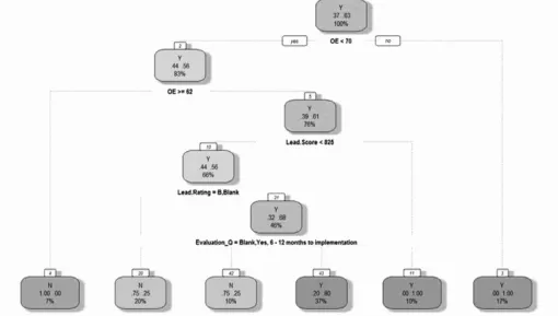
purpose of this study was to develop generalized rule based fuzzy models from multiple knowledge sources to test the hypothesis that high job demands and low job control (job strain) are associated with elevated free cortisol levels early in the working day and with reduced variability across the day and to evaluate the contribution of Anger Expression to this pattern and subsequently test its performance by comparing defuzzified outputs to actual values from test data and comparing predicted and actual fuzzy classifications. The overall approach followed in this study is illustrated in Figure 1. The process begins with knowledge acquisition, continues to model building and then finally testing the model performance. In the context of fuzzy modeling, the proposed approach of converting the predicted fuzzy output and the actual crisp value into fuzzy classification sets is not well defined in literature.

Each row of membership functions constitutes an IF– THEN rule, also defined by the user. Depending on the values used, the input membership functions are activated to a certain degree. The contributed output from each rule reflects this degree of activation. The final output is a fuzzy set created by the superposition of individual rule actions (Figure 1).

(3)

Fuzzy modeling of cortisol secretion of job strain Due to stress using extended hausdroff distances For intuitionistic fuzzy sets

-233-

2.1 DEFUZZIFICATION METHODS

The fuzzy output is obtained from aggregating the outputs from the firing of the rules. Subsequent defuzzification methods on the fuzzy output produce a crisp value. Two common techniques for defuzzification are the maxima methods and area-based methods, which are briefly explained. Several such methods are explained by Ross (1995).

3. DISTANCE MEASURES BETWEEN FUZZY SETS

For two fuzzy sets A and B in the same universe, the Hamming distance (HD) [5] is an ordinal measure of dissimilarity and is defined as:

∑

=

−

n i i B i

A

x

1

)

(

)

(

=

B)

HD(A,

μ

where n is the number of points that define the fuzzy sets A and B, μA(xi) the membership of point xi in

A and μB(xi) is the membership of point xi in B. The Hamming distance is smaller for fuzzy sets that are

more alike than those that are less similar.

3.1 ENTROPY OF A FUZZY SET

Entropy is a measure of fuzziness associated with a fuzzy set. The degree of fuzziness can be described in terms of a lack of distinction between a fuzzy set and its complement. For a fuzzy set A, entropy [6] is calculated as:

∑

=

−

n i i A

x

n

1

1 )

(

2

1 -1

=

E(A)

μ

………(1)

where n is the number of points that define A, and μA(xi) is the membership of point xi in A. In this

study, the concept of entropy was used to quantify the ambiguity associated with the predicted fuzzy outputs. In the absence of actual values, entropy values are essentially a measure of confidence in outputs predicted by a fuzzy model.

3.2 PROPOSED DISTANCE MEASURE

As indicated in the theory section, a modified form of the Hamming distance is proposed which enables better distinction between different levels of classification (see Table1 and 2).

The proposed distance measure D(A, P) is defined as:

) ) ( ) ( ) 1 2 ( 2 ( ) ( ) ( ( 4 1 = B) D(A, ) ( 1 , 1

∑

≠ = = − − + − n k i k i k P i A n i i B i

A x

μ

x i k

μ

x

μ

x

μ

……(2)

where A is the actual fuzzy classification, P the predicted fuzzy classification, n the number of classes that define A and P, μA(xi) is the membership of point xi in A and μP(xk) is the membership of point xk

in P.

3.3 COMPARING FUZZY CLASSIFICATIONS

(4)

-234-

the predicted fuzzy set over the range of the membership function. Equations (3) were used to develop the predicted fuzzy classification:

)

(

x

P

μ

=

∫

dx x

dx x x f

i i

) (

) ( .) (

μ

………….(3)

For each test case, an actual fuzzy classification and a predicted fuzzy classification were obtained. The modified Hamming distance measure (3) was used to determine the similarity between the two fuzzy sets. Apart from a comparison to actual values, the ambiguity associated with each predicted value was quantified using an entropy measure (1) as defined in the theory section.

3.4 DEFUZZIFYING THE PREDICTED OUTPUT

The centroid method was used to defuzzify the output of the Mamdani models. The crisp predictions were compared to the actual values from the test data and entropy value was calculated. This is a common form of comparison utilized for most modeling strategies. However, defuzzifying the output results in a loss of information regarding the ambiguity of the prediction. In the absence of actual values, the confidence in the prediction can be determined based on the degree of ambiguity.

3.5 INTUITIONISTIC FUZZY SETS

Intuitionistic fuzzy set was introduced first time by Atanassov, which is a generalization of an ordinary Zadeh fuzzy set. Let X be a fixed set. An intuitionistic fuzzy set A in X is an object having the form

, , | where the functions , 0,1 are the degree of membership and

the degree of non-membership of the element to , respectively; moreover, 0 1 must

hold.

Obviously, each fuzzy set may be represented by the following intuitionistic fuzzy set

, , 1 |

3.6 DISTANCE BETWEEN INTUITIONISTIC FUZZY SET

In Szmidt and Kacprzyk [7], [8], it is shown why in the calculation of distances between the intuitionistic fuzzy sets one should use all three terms describing them. Let A and B be two intuitionistic fuzzy set in

, , … ,

. Then the distance between A and B while using the three term representation (Szmidt and Kacprzyk) may be as follows.

The Hamming distance:

,

∑

|

The Euclidean distance:

,

∑

The normalized Hamming distance:

,

∑

|

The normalized Euclidean distance:

,

∑

3.7 THE HAUSDROFF DISTANCE

Given two intervals

,

and

,

_{of Intuitionistic fuzzy set, the hausdroff metric is defined [9],}

,

max |

|, |

|

. The hausdroff metric applied to two intuitionistic fuzzy sets,

, 1

and

, 1

, given the following:

(5)

-235-

The following two term representation hausdroff distances between intuitionistic fuzzy sets have been proposed [9]: The Hamming distance:

,

∑

max |

|, |

|

The normalized Hamming distance:

,

∑

max |

|, |

|

The Euclidean distance:

,

∑

,

The normalized Euclidean distance:

,

∑

,

The Extended haudroff - normalised Hamming distance:

,

∑

In comparing an actual fuzzy set to the predicted fuzzy set, a small Hamming distance is ideal. In our study, the model-testing phase involved comparison of predicted and actual fuzzy classifications (low and high). From the results in Table 1, the proposed distance measure is better than the Hamming distance at distinguishing between different levels of classification. In cases e and f, the Hamming distance(HD) gave the same value for different predicted fuzzy classifications[10]. The extended Hausdroff distance gave different values that effectively distinguish between these cases.

4. EXAMPLE

Data were collected at the 12-month follow-up phase of a study of job strain and cardiovascular risk, details of which have been published previously [10]. Participants in the original sample were 162 junior and high school teachers, selected on the basis of scores on a work stress measure (37) as having high (28 men and 52 women) or low (32 men and 50 women) job strain scores. Eighty-five (52.5%) were classroom teachers, and 77 (47.5%) had additional administrative roles. One hundred thirty-seven teachers took part in the 12-month phase (84.6%), which consisted of ambulatory blood pressure monitoring and a psychiatric interview (to be reported elsewhere) in addition to cortisol measurements. Of the 25 who did not participate at 12 months, 10 had left teaching or retired, 7 were seriously ill or pregnant, 1 experienced equipment failure, and 7 did not respond to our invitation. Comparisons between the 137 participants and 25 who dropped out of the study revealed no significant differences in gender, job strain scores, age, grade of employment, or scores on negative affect or anger expression. An additional 15 of the 137 individuals refused to sample saliva during the working day, mainly because they envisaged that data collection might be embarrassing or inconvenient at school. Statistical comparisons of these individuals with the remainder again identified no differences on demographic or psychological variables.

(6)

-236-

Figure 3. Mean concentration of saliva free cortisol in men and women across the day and evening. Fuzzy function of the given figure 2 and 3 is defined as

⎪

⎩

⎪

⎨

⎧

∈

+

−

∈

+

−

=

]

7 .

0 ,

4 .

0 [

,

9 .

0 ]

4 .

0 ,

2 .

0 [

,

5 .

0 ]

2 .

0 ,

0 [

,

5 .

1

5 )

(

x

f

⎪

⎩

⎪

⎨

⎧

∈

+

−

∈

=

otherwise

x

A

,

0 ]

4 .

0 ,

25 .

0 [

,

67 .

2

67 .

6 ]

25 .

0 ,

15 .

0 [

,

1 ]

15 .

0 ,

0 [

,

67 .

6 )

(

1

⎪

⎩

⎪

⎨

⎧

∈

+

−

∈

−

=

otherwise

x

A

,

0 ]

7 .

0 ,

5 .

0 [

,

5 .

3

5 ]

5 .

0 ,

4 .

0 [

,

1 ]

4 .

0 ,

2 .

0 [

,

1

5 )

(

2

Corresponding Fuzzy diagram are given in figure 4.

Figure 4. Fuzzy Mean concentration of saliva free cortisol in high and low job strain groups across the day and evening and Fuzzy Mean concentration of saliva free cortisol in men and women across the day and evening.

(7)

-237-

12:30, 14:00 to 14:30, 16:00 to 16:30, 18:00 to 18:30, 20:00 to 20:30, and 22:00 to 22:30 hours. The first sample of the day was always obtained at schools after explanation of the procedure by the investigators. Saliva samples were collected in Salivettes, which were stored at −30°C until analysis. After defrosting, samples were spun at 3000 rpm for 5 minutes, and 100 μl of supernatant was used for duplicate analysis involving a time-resolved immunoassay with fluorescence detection.

Case Actual fuzzy classification Predicted fuzzy classification HD Predicted Distance Time High

) ( i A x

μ Low μA(xi)

High ) ( i B x

μ Low μB(xi)

a 8 – 8.30 (1, 0) (0.83, 0.17) (0.9, 0.1) (0.8, 0.2) 0.13 0.43 b 10 – 10.30 (0.45, 0.55) (0.45, 0.55) (0.8, 0.2) (0.8, 0.2) 0.4 0.34 c 12 – 12.30 (0.39, 0.61) (0.39, 0.61) (0.5, 0.5) (0.5, 0.5) 0.16 0.13 d 14 – 14.30 (0.44, 0.54) (0.44, 0.54) (0.4, 0.6) (0.4, 0.6) 0.16 0.11 e 16 – 16.30 (0.31, 0.69) (0.31, 0.69) (0.5, 0.5) (0.5, 0.5) 0.4 0.18 f 18 – 18.30 (0.24, 0.76) (0.27, 0.73) (0.4, 0.6) (0.5, 0.5) 0.4 0.16 g 20 – 22.30 (0.17, 0.83) (0.21, 0.79) (0.4, 0.6) (0.5, 0.5) 0.51 0.18 Entropy Value (0.57, 0.43) (0.64, 0.36) (0.64, 0.36) (0.8, 0.2)

Various Distance Between Intuitionistic fuzzy set Women Men

Hamming Distance 0.54 0.55

Euclidean Distance 0.39 0.49

Normalized Hamming Distance 0.15 0.16 Normalized Euclidean Distance 0.15 0.19 Hausdorff Hamming Distance 0.53 0.54 Hausdorff Euclidean Distance 0.39 0.49 Hausdorff Normalized Hamming Distance 0.15 0.16 Hausdorff Normalized Euclidean Distance 0.15 0.19

Table 1: Comparison of the various distances of Fuzzy Mean concentration of saliva free cortisol in high and low job strain groups across the day and evening

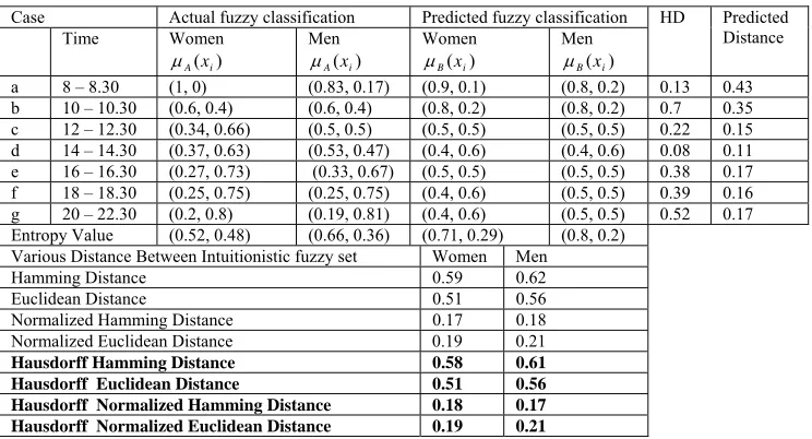
Case Actual fuzzy classification Predicted fuzzy classification HD Predicted Distance Time Women

) ( i A x

μ Men μA(xi)

Women ) ( i B x

μ Men μB(xi)

a 8 – 8.30 (1, 0) (0.83, 0.17) (0.9, 0.1) (0.8, 0.2) 0.13 0.43 b 10 – 10.30 (0.6, 0.4) (0.6, 0.4) (0.8, 0.2) (0.8, 0.2) 0.7 0.35 c 12 – 12.30 (0.34, 0.66) (0.5, 0.5) (0.5, 0.5) (0.5, 0.5) 0.22 0.15 d 14 – 14.30 (0.37, 0.63) (0.53, 0.47) (0.4, 0.6) (0.4, 0.6) 0.08 0.11 e 16 – 16.30 (0.27, 0.73) (0.33, 0.67) (0.5, 0.5) (0.5, 0.5) 0.38 0.17 f 18 – 18.30 (0.25, 0.75) (0.25, 0.75) (0.4, 0.6) (0.5, 0.5) 0.39 0.16 g 20 – 22.30 (0.2, 0.8) (0.19, 0.81) (0.4, 0.6) (0.5, 0.5) 0.52 0.17 Entropy Value (0.52, 0.48) (0.66, 0.36) (0.71, 0.29) (0.8, 0.2)

Various Distance Between Intuitionistic fuzzy set Women Men

Hamming Distance 0.59 0.62

Euclidean Distance 0.51 0.56

Normalized Hamming Distance 0.17 0.18 Normalized Euclidean Distance 0.19 0.21 Hausdorff Hamming Distance 0.58 0.61 Hausdorff Euclidean Distance 0.51 0.56 Hausdorff Normalized Hamming Distance 0.18 0.17 Hausdorff Normalized Euclidean Distance 0.19 0.21

Table 2: Comparison of the Hamming various distances of Fuzzy Mean concentration of saliva free cortisol in men and women across the day and evening.

Extended Hausdroff Distance

(8)

-238-

CONCLUSION

There were significant differences between groups in job strain and in its components job demands, job control, and skill utilization. The high job strain group reported greater demands, lower control, and less skill utilization than the low job strain group as inputs. Negative affect was significantly higher among high job strain individuals, and in scores were also greater. There were no differences in anger-out ratings between groups. Using multiple knowledge sources, membership functions and rules were developed to provide generalized models not optimized for a specific data set. Apart from correlation estimates of actual and defuzzified predictions, an alternative analysis was performed involving comparison of actual and predicted fuzzy classifications. Various distances measure were used to compare actual and fuzzy classifications. The extended hausdroff distance often used to compare distances between fuzzy sets.

REFERENCES

1. Zadeh L. A. (1965) Fuzzy sets, Information and Control, 8 pp 338-353.

2. Attanasov K(1999) Intuitionistic fuzzy sets: Theory and Applications. Physica-Verlag, Heidelberg and New York.

3. Ross T. J, Fuzzy Logic with Engineering Applications, Mc- Graw-Hill Inc., New York, 1995.

4. Hung W, A note on entropy of intuitionistic fuzzy sets, Int. J. Uncert. Fuzz. Knowledge-Based Syst. 11 (2003) 627–633.

5. Szmidt E., Kacpryzk J., Distances between intuitionistic fuzzy sets, Fuzzy Sets Syst. 114 (2000) 505–518. 6. Pham D.T, Castellani. M, Action aggregation and defuzzification in Mamdani-type fuzzy systems, in:

Proceedings of the Institute of Mechanical Engineers Part C, J. Mech. Eng. Sci. 216 (2002) 747– 759.

7. Eulalia Szmidt and Janusz Kacprzyk, Intuitionistic fuzzy sets – two and three term representation in the context of a Hausdroff distance, Acta Universitatis Matthiae Bell11, series Mathematics 19 (2011) 53-62. 8. Szmidt.E and Kacprzyk J (2000) Distance between intuitionistic fuzzy sets. Fuzzy sets and systems, 114(3),

505-518.

9. Grzegorzewski, (2004) Distances between intuitionistic fuzzy sets and / or interval- valued fuzzy sets based

on the hausdroff metric. Fuzzy Sets and Systems, 48:319-328,2004.

10. P. Senthil Kumar, B. Mohamed Harif, (2014) Rule-based Mamdani-type Fuzzy Modeling of perceived stress, and cortisol responses to awakening, IJERA, vol.4, 29-35.

(9)

-239-

A RELIABILITY MODEL ON A CEMENT GRINDING SYSTEM WITH

FAILURE IN ITS NINE COMPONENTS

Ritu Gupta*

& Dr. Gulshan Taneja**

* Research Scholar, Department of Mathematics, M.D. University, Rohtak, Haryana ** Professor, Department of Mathematics, M.D. University, Rohtak, Haryana

Email : [email protected], [email protected]

ABSTRACT :

The present study investigates the reliability and profit analysis of a cement grinding system with failure in the nine important components namely; Belt Conveyor, Bucket Elevator, Separator, Roller Press, Diverting Gate, Process Fan, Cyclone, Ball Mill and Fly Ash System. Only one type of failure has been considered in each of these components except that in the Diverting Gate. In Diverting Gate, two types of failure- minor and major has been taken into consideration. Also in case of Fly Ash System, occurrence of failure does not always results to the failure of the complete system. Data on failure times and cost of repairs have been collected from Shree Cement Ltd., Khushkhera, Rajasthan, India. The system has been analysed by using semi – Markov processes and regenerative point technique. Mean Time to System Failure (MTSF) and various other measures of system effectiveness have been obtained. Profit is also evaluated and graphical study is made to draw various important conclusions.

Keywords: Reliability, Cement Grinding System, Measures of System Effectiveness, Profit Analysis.

1. INTRODUCTION

Researchers’ both from academia and industries have developed a number of reliability models and analysed various measures of system effectiveness. Mokaddis et al. [1997] discussed cost analysis of two dissimilar unit cold standby redundant system subject to inspection and two types of repair. Parashar and Taneja [2007] discussed the reliability and profit evaluation of a PLC hot standby system based on master-slave concept and two types of repair facilities. Goyal et al. [2009]developed a model for a 2-unit cold standby system working in a sugar mill with operating and rest periods. Mathew et al. [2009] discussed profit evaluation of a single unit CC plant with scheduled maintenance. Padmavathi el al. [2012] discussed reliability analysis of an evaporator of a desalination plant with online repair and emergency shutdown. Sharma and Gupta [2012] discussed cost benefit analysis of three unit redundant system model with correlated failures and repairs. Hashim et al. [2013] discussed reliability analysis of phased mission system considering the concept of sensitivity, uncertainty and common cause failure using the GO-FLOW methodology. Jain et al. [2013] analysed a two unit automatic power factor controller system with inspection and four types of failure. Taneja G and Singh Dalip [2013] discussed reliability analysis of a power generating system through gas and steam turbines with scheduled inspection.

(10)

Ritu Gupta & Gulshan Taneja

-240-

Cement is an important constituent of concrete which is an essential material for construction in modern infrastructure. The grinding of cement clinker is an intermediate step in cement manufacturing process. On the basis of data/information gathered from Shree Cement Limited, India, the study investigates the reliability and cost-benefit analysis of the cement grinding process. The cement grinding system comprises mainly the following nine components namely:

(1) Belt Conveyor (2) Bucket Elevator (3) Separator (4)Roller Press (5) Diverting Gate (6) Process Fan (7) Cyclone (8) Ball Mill (9) Fly Ash System

Diverting gate is the component for which two types of failure – minor and major have been observed and hence considered. Minor failure leads to partial failure due to which system does not become inoperable i.e. it still works whereas a major failure leads to complete failure of the system. On occurrence of the failure in fly ash system, it does not go to failed state immediately and may remain operable for some stipulated time period during which the efforts may be made to remove or repair the faults. However, if the faults are not removed within the stipulated time period, the system becomes inoperable i.e. goes to failed state. Various measures of the system effectiveness and reliability characteristics such as mean time to system failure (MTSF), availability, expected number of replacements or repairs of the nine components, expected number of visits by the repairman and profit function are evaluated in steady state using semi-Markov processes and regenerative point technique. Various important conclusions have been drawn from the graphs plotted for the model

NOTATIONS

O : cement grinding system is operative

λi : constant failure rate of ith component of the system; i = 1,2,...,9

G i(t), gi(t) : cdf and pdf of repair time of ith component; i = 1,2,3,4,6,7,8,9

p1, q1 : probability of minor and major leakage in diverting gate

G51(t), g51(t) : cdf and pdf of repair time for minor leakage in diverting gate.

G52(t), g52(t) : cdf and pdf of repair time for major leakage in diverting gate.

p2 : probability that failure in fly ash system is repaired before the fly ash in the bin is consumed

completely

q2 : probability that fly ash in the bin is consumed completely but the component is not repaired

I(t), i(t) : pdf and cdf of allowable time during which dry fly ash is there in the bin. Fri : completely failed ith component under repair; i = 1,2,...,9

pfr5 : partially failed 5th component under repair

Oir : online repair is going on after the failure of fly ash system but within the stipulated time

qij(t), Qij(t) : probability density function (p.d.f.), cumulative distribution function (c.d.f.) of first passage time

from a regenerative state i to a regenerative state j without visiting any other regenerative state in

(0,t]

Ai(t) : probability that the system is in up state at the instant t given that the system entered regenerative

(11)

A Reliability model on a cement grinding system with failure in its nine components

-241-

ERij(t) : expected number of replacements/repairs in jth component at instant t given that the system started

from the regenerative state i at t=0; j= I,II,...,X

Vi(t) : expected number of visits of the repairman in (0,t] given that the system entered regenerative state i

at t=0

Transition Probabilities and Mean Sojourn Times:

A transition diagram showing the various states of the system is shown in Fig.1. The epochs of entry into states 0 to 11 are regeneration points and hence these states are regenerative states. States 0, 5 and 10 are up states. States 1 to 4, 6 to 9 and 11 are failed states. The non zero elements pij = lim

q

ij

*

(

s

)

are given below:

p0j = ( j= 1,2,3,4)

p05 =

p06 =

p0j = ( j=7,8,9,10)

pi,0=1 (i=1,2,...9)

p10,0=p2

p10,11=q2

p11,0 =1

By these transition probabilities, it can be verified that and

∑

=

9 1

5 1

i i

p

λ

∑

=

9 1

5 1

i i

q

λ

∑

=

9 1 i

i

j

λ

∑

= −

9 1

1

i i j

λ

1 ,

1 ₁₀_,₀ ₁₀_,₁₁ 10

1 0,

= +

=

∑

=

p p p

j j

)

9 ,...,

2 ,

1 (

1 ,

1

_,₀

0 ,

11

=

p

=

i

=

(12)

-242-

The mean sojourn time ( ) in state i is given by:

The unconditional mean time taken by the system to transit for any regenerative state j when the time is counted from epoch of entrance into state i is given as:

Thus,

MEASURES OF SYSTEM EFFECTIVENESS

Various measures of system effectiveness obtained in steady state using the arguments of the theory of regenerative process are:

(1) The Mean Time to System Failure (MTSF) = N/D (2) The Availability of the System (A0) = N1/D1

=

0

μ

∑

∫

= ∞ _⎟⎟ ⎠ ⎞ ⎜ ⎜ ⎝ ⎛ −

=

∑

= 9 1 0

1

9 1 i i t

dt

e

i i

λ

)

4 ,

3 ,

2 ,

1 (

),

0 (

*'

=

−

=

g

_k

k

μ

)

0 (

*'

),

0 (

*'

₆ ₅₂

51

5

=

−

g

μ

=

−

g

μ

)

0 (

*'

),

0 (

*'

),

0 (

*'

),

0 (

*'

),

0 (

*'

9 11 10 8 9 7 8 6 7

g

i

g

−

=

−

=

−

=

−

=

−

=

μ

∫

∞ = 0 ) (t dt tq mij ij

11 0 , 11 10 11 , 10 0 , 10 0 , 10

1 0, 0

, ), 9 ,...., 2 , 1 ( ,

μ

= = + = = =

∑

= m m m i m

m _i _i

j j

(13)

-243-

(3) Expected Number of Replacements/Repairs of parts in Belt Conveyor: ER0I = N2 / D1

(4) Expected Number of Replacements/Repairs of parts in Bucket Elevator: ER0II = N3 / D1

(5) Expected Number of Replacements/Repairs of parts in Separator: ER0III = N4 / D1

(6) Expected Number of Replacements/Repairs of parts in Roller Press: ER0IV = N5 / D1

(7) Expected Number of Replacements/Repairs of parts in Diverting Gate on Minor Failure: ER0V = N6 / D1

(8) Expected Number of Replacements/Repairs of parts in Diverting Gate on Major Failure: ER0VI = N7 / D1

(9) Expected Number of Replacements/Repairs of parts in Process Fan: ER0VII = N8 / D1

(10) Expected Number of Replacements/Repairs of parts in Cyclone: ER0VIII = N9 / D1

(11) Expected Number of Replacements/Repairs of parts in Ball Mill: ER0IX = N10 / D1

(12) Expected Number of Replacements/Repairs of parts in Fly Ash System: ER0X = N11 / D1

(13) Expected Number of Visits by the Repairman (V0) = N12/D1

where

N2 = p01, N3 = p02 , N4 = p03, N5 = p04 , N6 = p05 , N7 = p06 , N8 = p07 , N9 = p08 , N10 = p09 ,

N11 = p0,10 ,

0 , 10 10 , 0 05

1 p

p

D

=

−

D1 = μ0 + ∑ + μ11 p0,10 p10,11

PROFIT ANALYSIS

Expected profit incurred to the system is given as:

P = C0A0 - C1ER0I - C2ER0II - C3ER0III - C4ER0IV - C5ER0V- C6ER0VI - C7ER0VII - C8ER0VIII -

C9ER0IX -C10ER0X - C11V0

where

C0 = revenue per unit up time of the system

C1 = cost per replacement/repair of parts in Belt Conveyor

C2 = cost per replacement/repair of parts in Bucket Elevator

C3 = cost per replacement/repair of parts in Separator 10

10 , 0 5 05

0

μ

p p

N = + +

1

0 10

1 12

=

∑

=

= i

i

p

N

10 10 , 0 5 05 0

1

μ

p

μ

p

μ

(14)

-244-

C4 = cost per replacement/repair of parts in Roller Press

C5 = cost per replacement/repair of parts in Diverting Gate on minor failure

C6 = cost per replacement/repair of parts in Diverting Gate on major failure

C7 = cost per replacement/repair of parts in Process Fan

C8 = cost per replacement/repair of parts in Cyclone

C9 = cost per replacement/repair of parts in Ball Mill

C10 = cost per replacement/repair of parts in Fly Ash System

C11 = cost per visit of the repairman

RESULTS AND DISSCUSSION

The following particular case is consideredfor graphical study: gi (t) = i t

i

e

α

− _{, i =1,2,...,9 , i}_≠₅

g51 (t) =

t

e

51 51

α

−

, g52 (t) =

t

e

52 52

α

−

, i(t) = t

e

β

−

The following values have been estimated from the gathered data/information:

λ1=0.0004235, λ2=0.0005802 , λ3=0.0003948 , λ4=0.0008738 , λ5=0.0008158 ,λ6=0.0002789, λ7=0.0004236 ,

λ8=0.0003778 , λ9=0.0002783 , α1=0.1892333 , α2=0.0871105,α3=0.0666667, α4=0.0993984 , α51=0.2692308 ,

α52=0.1165049, α6=0.097643 , α7=0.0862069, α8=0.0453258 α9=0.1164902 , β=3, p1=0.5392 , q1=0.4608 , p2=0.1 ,

q2=0.9 , Co=1540 , C1=55495.69 , C2=105689.43 , C3=15161.76 , C4=1442167.1 , C5=339.29 , C6=1075,

C7=11020.69 , C8=25280 , C9=211525 , C10=17536.36 ,C11=20000

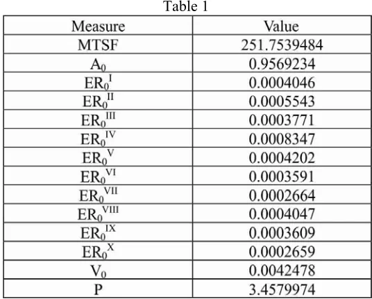
Using the above estimated values, the following measures of system effectiveness are obtained:

Table 1

(15)

-245-

CONCLUSION

Following conclusions are drawn on the basis of the graphs, irrespective of the fact whether they are being shown here or not:

• The MTSF and Availability gets decreased as the failure rate (λ5) increases and also gets lowered for higher

values of failure rate (λ9).

(16)

-246-

REFERENCES

1. Parashar B and Taneja G (2007) “Reliability and Profit Evaluation of a PLC Hot Standby System Based on a Master Slave Concept and Two Types of Repair Facilities”, IEEE Transactions on Reliability, 56(3), 534-539.

2. Goyal A, Taneja G and Singh D V (2009) “Analysis of a 2-Unit Cold Standby System Working in a Sugar Mill with Operating and Rest Periods”, Caledonian J. Engg., 5(1), 1-5.

3. Mathew A G, Rizwan S M, Majumdar M C, Ramachandran K P & Taneja G (2009)“ Profit Evaluation of a Single Unit CC Plant with Scheduled Maintenance”, Caledonian journal of Engineering; 5: 1-5

4. Padmavathi N, Rizwan S M, Pal Anita and Taneja G (2012)“Reliability Analysis of an Evaporator of a Desalination Plant with Online Repair and Emergency Shutdown”, Aryabhatta Journal of Mathematics & Informatics, 4(1), 1-12. 5. Sharma V K and Gupta S P (2012)“Cost Benefit Analysis of Three Unit Redundant System Model with Correlated

Failures and Repairs”, Journal of Pure and Applied Science & Technology,Vol.2(1),pp1-10.

6. Hashim M, Hidekazu M T, Ming Yang (2013) “Reliability Analysis of Phased Mission System by Considering the Concept of Sensitivity Analysis, Uncertainty Analysis and Common Cause Failure Analysis using the GO-FLOW Methodology”, Research Journal of Applied Sciences, Engineering and Technology Vol. 5 No.12, 3465-3475.

7. Jain Roosel, Taneja G and Bhatia P K (2013) “Analysis of a Two Unit Automatic Power Factor Controller System with Inspection and Four Types of Failure” , Advanced Modelling and Optinization (AMO)”, 15, 487-497.

(17)

-247-

A GENERALIZED DOUBLE ENDED STOCHASTIC QUEUE

SYSTEM WITH EXCESS CUSTOMER DEMAND IN REAL

WORLD SITUATIONS

Reeta Bhardwaj, T. P. Singh and Vijay Kumar

* & ***Assistant professor, Department of Mathematics, Amity University, Punchgaon, Manesar, Gurgaon (India) **Professor, Department of Mathematics, Yamuna Institute of Engg. & Technology, Gadholi, Yamuna Nagar (India)

Email: - [email protected]*,[email protected]**, [email protected]***

ABSTRACT :

A double ended queue model is a system where customer demanding and resource supply arrive to a work station in poisson process. When there is a pair of customer and resource in a system, they immediately transact the required system and leave the system. Thus, there cannot be non-zero numbers of customers and resources simultaneously in the system.

The double ended queue system can be applied to model various social and economic situations in real world scenario. We analyzed the various queue parameters like mean queue length, waiting time and the cost functions etc. due to imbalance of customer demand and resources. The analysis has been made analytically. The queuing behavior in different situations has been examined and a comparative study has been made with the work already done through simulation. The main objective of the paper is to explore the situation when the stochastic system becomes unstable due to excess customers. The effect of customer's reduction factor and resource expansion factor has been examined graphically. The limitations of the model has also been given and extensions are suggested.

Key Words: Double ended, Poisson process, customer reduction factor, resource expansion factor.

1. INTRODUCTION

Stochastic model provides the basic frame work for analyzing the natural as well as socio-economic phenomenon in real world context. The analysis of double ended queue system has attracted the attention of several investigators. Kendall [1951] was the first who discussed the double ended queue problem in which the passengers and taxis arrive at a taxi stand in Poisson’s stream with constant mean rate

λ

and

μ

_{. No limit was placed on the numbers of} passengers or taxis that can form a queue at the stand. Kashyap [1966] considered the double ended queue with limiting waiting space for both passengers and taxis with Poisson arrival. Perry and Staje [1999] explored an inventory system for perishable commodities with finite shelf size and finite waiting room, for demand units. Conolly and Parthasarathy[2002] studied the effect of impatient behavior of customers in the context of double ended queue. Mendoza, Sedaghat and Yon [2009] developed an optimization model for the double ended queue due to imbalance of supply. Kim et al [2010] developed a simulation design for extended double ended queue model and studied sensitive analysis on performance measures by changing parameters and impact factors such as batch size, processing time, probability of paring failure etc.Arti and Singh T.P. [2014] through his case study showed that how queuing theory satisfies the stochastic model when applied in real time scenario.

(18)

Reeta Bhardwaj, T. P. Singh & Vijay Kumar

-248-

demand/supply system where demand and supply queues both have finite maximum possible lengths. These authors generated a number of scenarios using Monte Carlo’s technique and the results obtained in these scenarios are used to find regression equations that express the policy factor.

Along with the research line traced by above mentioned researchers, we present the double ended stochastic queue model in general form with excess customers may be considered as excess demand queue in the sense of Mendoza et al [2014]. An effort has been explored to find an optimal policy in these situations. The analysis has been made mathematically rather than simulation. The model parameters affecting the optimal value of policy factors have been analyzed mathematically & graphically. The effect of changing the reduction factor on mean queue length with excess customer demand queue and excess resources supply queue has been presented in tabular form and the comparative study with discouraged customers or excess resources has been made. A graphical analysis has been made and is compared with the simulation study done by Mendoza et al [2014].We present numerical results for the model at the resource level and customer level. We address four questions (i). What is the general behavior of these matrices? (ii) What are the sensitivities on changing the parametric value? (iii) How do the system level matrices compared with the results given by simulation study? (iv) How do the customer level matrices compared with those given by simulation? Limitations of the model and further scope of the research has also been highlighted in this paper.

Following, the introductory part and the literature survey, the remainder of the paper proceeds as follows. In section 2, we present the social and economic situations where the model can be applied. In section 3, the model has been framed with relevant notations.Section 4 derived the steady state equations for the model and its stability conditions and provides formulae for system expected performance. Various queue characteristics for both customers and resources have been derived along with reduction factor in section 5. Some of these results are known while some are new. In section 6, we derive matrix on the performance of the system for excess customer demand queue and makes an analytic study of cost parameter due to excess customers. The results for model have been compared with the simulation study already made by Mandoza etal [2014] in Section 7. We discuss our results in section 8 and present further scope in research direction.

2. APPLICATION OF THE MODEL IN SOCIAL AND ECONOMIC SITUATION

(19)

A Generalized Double Ended Stochastic Queue System with Excess Customer Demand in Real World Situations

-249-

We also find that in research funding cases which are obtained through a competitive process, the excess research scholars can be supposed in form of demanding unit for fellowships or funds. The potential research proposals are evaluated in R&D department and only some of the most promising proposals receive funding. The researchers request to a granting agency may be UGC/CSIR for financially support their proposals. We can assume proposals request for sponsorship or fellowship or funding, follow a Poisson process.

We find a very practical situation of double ended queue system in ware housing. Automatic storage and retrieval systems (AS/RS) are widely used in ware houses. AS/RS using a queue model with two linked queues, one for the items waiting for storage and other of finite capacity for the request for an item to be removed from storage based on the size of storage racked can be supposed as an example of a double ended queue. Queue 1 is considered to be arrival queue, where items wait to be placed into storage, queue 2 is considered to be the queue in which the request for retrieval is arrived. Queue 2 is depended on the numbers of racks.

3. THE MODEL

We present a general double ended stochastic queue model in which the customers and commodity (resources) queue have maximum possible length K1 and K2 respectively with the state of system one dimensional index.

Customers arriving in a group may be taken as one unit assuming that a group does not consist of more customers than the capacity of resources. Excess resource results in a positive index while excess customers result in negative index i.e,

0

n> Indicates numbers of resources are waiting. 0

n= Indicates neither resources nor customers are waiting. 0

n< Indicates – n customers are waiting. The numerical value gives the customers waiting.

(20)

-250-

also find the effect of reduction factor causes due to customer demand queue on expected queue length. The cost analysis due to imbalance of excess customer demands queue and resources have been discussed mathematically in detail.

Notations

λ- Average rate of resources µ-Average rate of customers

α

– Customers reduction factor

αμ

– New customer reduction factor in which 0< <

α

1

ρ

– Utilization factor

λ

αμ

=

(due to excess customers)

β

– Resource expansion factor

λβ

– New resource expansion factor in which

β

>1

ρ

– Utilization factor

λβ

μ

=

(due to excess resources)

1

C

– Cost per unit time of one unit of excess customers in the queue

2

C

– Cost per unit time of one unit of excess resources in the queue

C

_α– Cost incurred per time unit in reducing the customer rate by one unit

1

K

– Mean length of customers queue.

2

K

– Mean length of resources queue.

4. STEADY STATE EQUATIONS OF THE MODEL DUE TO EXCESS CUSTOMERS

The transient analysis of queuing system is not always easy to be performed and it leads very often to non-manageable mathematical formulae. Hence it is feasible to study the system under consideration in steady state.

Let

P

_n be the steady state probability that the system is in state n here,

1

,

1

1,...0,1, 2...,

2

1,

2

n

= − − +

k

−

k

.The differential difference balance equation for steady state with customer reduction factor α due to excess customers can be summarized as follows:

1 1 1

k k

P

λ

−

=

αμ

− + (1)

1 1

(

λ αμ

+

)

P

n

=

λ

P

n−

+

αμ

P

n+ (2)

2 1 2

k k

P

λ

−

=

α

(3)

Solution Methodology From equation (1)

1 1 1

k k

P

λ

α μ

ρ

+ +

− −

=

_where

_ρ

λ

αμ

=

1 1 1

2

2 1

k k k

P

_{− +}

=

ρ

P

_{− +}

=

ρ

P

₋

1 1

3 3

k k

(21)

-251-

1 1

n

k n k

P

_{− +}

=

ρ

P

₋ (4)

In general,

P

_n

=

ρ

k1+n

P

₋_k₁

On applying the normalized condition 2

1

k

n n k

P

=−

=

∑

(5)

1 1 1

...

0 1

...

2

1

k k k

P

₋

+

P

_{− +}

+

P

+

P

+

P

=

1 2 1

2

1 ...

k k

1

k

P

₋

⎡

_⎣

+ +

ρ ρ

+

ρ

+

⎤

_⎦

=

Which on simplification

1 1 2 1

(1

)

1

k k k

P

ρ

− + +

−

=

−

(6)

From (4) we get,

(7)

5. QUEUE CHARACTERISTICS/PERFORMANCE MEASURES:

Obtaining performance measures is essential in order to utilize our queue model in redesign of the system. Further these performance measures allow us to determine how system is behaving on applying the reduction factor with excess customer demand queue.

Comparison on these performance measures for various value of the reduction factor will provide insight into what changes would be appropriate for the given conditions. The model can also be applied to determine the behavior of system and ultimately helps in deciding best optimal policy for the system.

5.1

Probability that waiting space is empty 1

1 2 1

0

1 2

(1

)

1

k

k k

if

P

if

k

ρ ρ

_ρ

ρ

+ +

⎧ −

_≠

⎪ −

⎪

= ⎨

⎪

₌

⎪ + +

(22)

-252-

5.2

Probability that there is queue of resources

(

2

)

1

2 ₁ ₂

1 1 1 ₂ 1 2

1

k k

k _k _k

r n

if

P

k

if

k

ρ

+ + +

⎧ −

⎪

≠

⎪

−

=

_{= ⎨}

⎪

₌

⎪

₊

⎩

∑

5.3

Probability that there is queue of customers

(

1

)

1 2 1 1 1 1 1 2

1

k k k c n k

if

P

k

if

k

ρ

− + + −

⎧

₋

⎪

≠

⎪ −

=

_{= ⎨}

⎪

₌

⎪ + +

⎩

∑

5.4

The mean queue length of resources

(

)

(

)

(

)

(

)

(

)

1 2 2

1 2 2 1 1 2 2 1 1 2 2 1 2

1

2

1

k k k

k k k r n

k

if

L

nP

k

if

k

ρ

+ + + +

⎧

⎡

_⎣

−

+

⎤

_⎦

⎪

≠

−

⎪

=

_{= ⎨}

+

⎪

=

⎪

₊

⎩

∑

5.5

The mean queue length of customers

(

)

(

)

(

)

(

)

(

)

1 1 2 1 1 1 1 1 1 1 1 1 2

1

2

1

k k k c n k

k

if

L

nP

k k

if

k

ρ ρ

ρ

+ + + − −

⎧ −

+

≠

⎪

−

⎪

=

−

_{= ⎨}

+

⎪

₌

⎪

₊

⎩

∑

5.6

Probability that resources are lost due to limiting waiting space

2

k

P

=

5.7

Probability that customer sare lost due to limiting waiting space

1

k

P

₋

=

5.8

Mean number of resources lost per unit time

2

k

P

λ

=

5.9

Mean number of customers lost per unit time

1

k

P

μ

₋

=

5.10

Mean waiting time for resources r r

L

W

λ

(23)

-253-

5.11

Mean waiting time for customers c c

L

W

λ

=

6. ANALYTICAL STUDY OF QUEUE PARAMETERS

When customers demand become higher than the resource parameter we have only two possibilities (i) either discourage the excess customers demand (ii) or increase the resource. In either the cases the mean queue length and other queue parameter will be affected and a cost will be associated in balancing and optimum decision depending upon the total cost selecting any one of these options.

Case 1: Balancing the system by reducing excess demands (A):Mean queue length due to excess customers.

Let

L

_c be the mean queue length due to excess customer.

α

is considered as customer reduction factor so that the new customer rate in terms of demand rate become

αμ

(0 <

α

<1).

From parameter 5.5, we find the following values of mean queue length due to excess customers, on applying a customer reduction factor

α

(0 <

α

<1). The different values are calculated mathematically and are presented in the following table for two different sets.

(24)

-254-

GRAPHICAL ANALYSIS

The mean queue length in the system, for customer queue and resource queue has been presented graphically. The graph shows that as, the customer reduction factor is greater than 1, the queue length grows higher and almost becomes constant. In this case, the asymptotes of the curve shifted to left indicating that the system gets unstable faster, since the resource rate is lesser. When the reduction factor is less than 1, the mean queue length is comparatively lesser but grows highly. At a reduction factor about 0.6, the queue length is minimum. It is because of high utilization of the service pattern depending upon the excess customer arrival rate and the resource rate. Low utilization would indicate that there is a room for increasing the use of storage facility. Hence, a smaller reduction factor would be more efficient. High utilization would indicate the system is being used efficiently. However, there is a little scope for increasing utilization. It creates instability in the system therefore reduction factor can’t be taken greater than 1.

(B):Cost parameters due to excess customer

In this study, we focus our attention mainly on practical and social situations where customers or demand factor is higher than the resources or supply factors i.e.,

μ λ

>

Let

C

₁be the cost per time unit of one unit of excess customer or demand for service in the queue.

C

₂be the cost per time unit of one unit of excess resources or supply in the queue.

α

is considered as customer reduction factor so that the new customer rate in terms of demand rate become

αμ

(0 <

α

<1) and

C

_αbe the cost incurred per time unit in reducing the customer rate by one unit. Let

P

_nbe the steady state probability that the system is in state

n

where

n

= − − +

k

₁

,

k

₁

1,...0,1, 2...

k

₂.

The expected total cost when a customer reduction factor is taken into consideration is given by

( )

2

1 1 1 2 1

(1

)

k n n

n k n

C

α

C

nP

C

nP

C

_α

μ

α

−

=− =

=

∑

−

+

∑

+

−

₍₈₎

First summation indicates expected under resource cost, second summation represents over resource cost and third term is expected cost of reducing the customers (either by increasing the fare price or redesigning the queue system) rate from

μ

to

αμ

in order to balance the system.

Substitute the value of

P

_nfrom (4) in (8), we get

( )

(

)

(

)

(

)

(

)

(

)

(

)

(

)

1 1 1 2 1 2

1 2 1 1 1 2 2 2

1 2

1 1 1 2

1 1 1 2 2 2

1

1 1

(1 ) 1

2 1

1

1 1

(1 ) 1

k k k k k k

k k

c k k c k k

C when

k k

c k k c k k

C C when α α

μ

α

ρ

ρ ρ

ρ

α

ρ

μ

α

ρ

+ + + + + + + + ⎧ ⎡_⎣ + + + ⎤_{⎦ +} − = ⎪ + + ⎪ ⎪₋ _{− + +} ₋ ₊ _⎡ _{− +} ₊ _⎤ = ⎨ ⎣ ⎦ ⎪ ₋ ₋ ⎪ ⎪+ − ≠ ⎩ (9) (10)

Where,

(

1 1

)

1 1

(

)

1 2 1 1 2 2

1( ) 1 1 1 2 1 2 2

k k k k k k

f

ρ

= −c − + +k

ρ

k

ρ ρ

− + +c ⎡_⎣

ρ

+ − +k

ρ

+ + +k

ρ

+ + ⎤_⎦

(

)

(

1 2 1

)

2

( )

1

k k

f

ρ

= −

ρ

−

ρ

+ +

(25)

-255-

OPTIMAL ANALYSIS

We find the following values that minimize the expected total cost on applying a customer reduction factor

α

(0 <

α

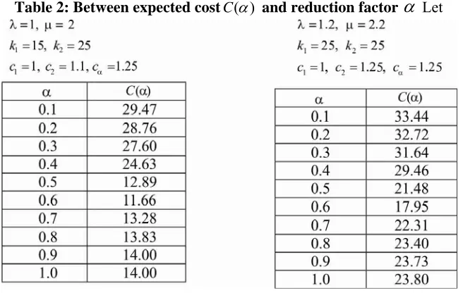
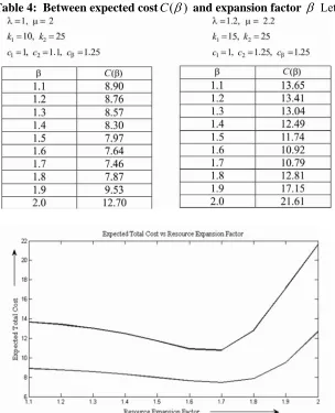
<1). The different values are calculated mathematically and are presented in the following table for two different sets.

Table 2: Between expected costC( )α and reduction factor

α

Let

The above tabular values has been presented in graphs between

α

and ( )C α

The graph shows the typical shapes of the relation-ship between minimum expected total cost C( )

α

and customer

reduction factor

α

. We find in most cases thatC( )

α

has two inflection points when

α

lies between 0 and 1. When

α

is 1 or more the value of C(1)is higher than the minimum. When

α

≥1either the customer demand should be

(26)

-256-

the least cost model for both cases i.e., case of expected mean queue length of customers as well as in expected total cost, as this value attains the high utilization of the system.

The formula can be used numerically to find the policy factor that would minimize the total expected cost in order to balance the queuing system. By comparing the minimum total expected cost, with the help of graph either by discouraging customers or by increasing resources is the best policy.

Case ii: Balancing the system by increasing resources (A):Mean queue length on increasing the resources

In this the rate of customer demand remains unchanged and we introduce the resource expansion factor

β β

( >1)

so that the utilization factor

ρ

λβ

μ

=

.

r

L

be the mean queue length on increasing the resources.

Steady state differential equations can be expressed as

1 1 1

k k

P

λβ

−

=

μ

− + (11)

1 1

(

λβ μ

+

)

P

n

=

λβ

P

n−

+

μ

P

n+ (12)

2 1 2

k k

P

λβ

−

=

μ

(13)

On solving, we get the similar results as already given in section 4 and queue characteristic will also be the same as given in section 5. From parameter 5.4, we find the following values of mean queue length on increasing the resources, on applying a resource expansion factor

β

(

β

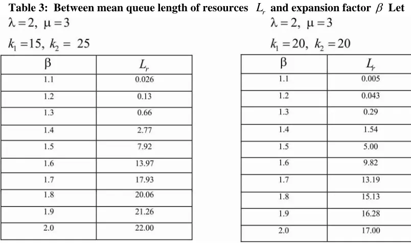
>1). The different values are calculated mathematically and are presented in the following table for two different sets.

Table 3: Between mean queue length of resources

L

_r

and expansion factor

β

Let

(27)

-257-

In case, if resource expansion factor is increased, the curve increases exponentially and the system become unstable faster.

(B): Cost parameters on increasing the resources

C

_β be the cost incurred per time unit in increasing the resource rate by one unit. Here the expected cost becomes:

( )

2

1 1 1 2 1

(

1)

k n n

n k n

C

β

C

nP

C

nP

C

_β

λ β

−

=− =

=

∑

−

+

∑

+

−

₍₁₄₎

First summation indicates expected under resource cost, second summation represents over resource cost and third term is expected cost of increasing the resource rate from

β

to

λβ

After putting

P

_nfrom equation (7) in equation (14) the expected total cost to the system, when resource expansion factor is applied, is given by

( )

(

)

(

)

(

)

(

)

(

)

(

)

(

)

1 1 1 2 1 2

1 2

1 1 1 2 2 2

1 2

1 1 1 2

1 1 1 2 2 2

1

1 1

( 1) 1

2 1

1

1 1

( 1) 1

k k k k k k

k k

c k k c k k

C when

k k

c k k c k k

C C when β β λ β ρ ρ ρ ρ ρ ρ ρ α ρ ρ λ β ρ + + + + + + + + ⎧ ⎡_⎣ + + + ⎤_{⎦ +} − = ⎪ + + ⎪ ⎪₋ _{− + +} ₋ ₊ _⎡ _{− +} ₊ _⎤ = ⎨ ⎣ ⎦ ⎪ ₋ ₋ ⎪ ⎪+ − ≠ ⎩ (15)

Where,

(

1 1

)

1 1

(

)

1 2 1 1 2 2

1( ) 1 1 1 2 1 2 2

k k k k k k

f

ρ

= −c − + +k

ρ

k

ρ ρ

− + +c ⎡_⎣

ρ

+ − +k

ρ

+ + +k

ρ

+ + ⎤_⎦

(

)

(

1 2 1

)

2( ) 1 1

k k f

ρ

= −

ρ

−

ρ

+ +

We find the following values that minimize the expected total cost on applying a resource expansion factor

β

(

β

>1). The different values are calculated mathematically and are presented in the following table for two

(28)

-258-

Table 4: Between expected costC( )

β

and expansion factor

β

Let

The minimum value of C( )

β

occurs for

β

>1 and has been presented graphically. We have shown the parametric

value for some fix value and it has found that in most of the cases the minimum cost C( )

β

occurs at

β

>1 and (1)

C is higher than the minimum.

In a nut shell, the formula can be used to find numerically the policy factor that would be minimized the total expected cost to balance the unbalancing queue system either by increasing the resources or decreasing the customer demand. The best policy is one which leads to the smallest expected unitary cost

7. CUSTOMER LEVEL COMPARISON TO A SIMULATED MODEL

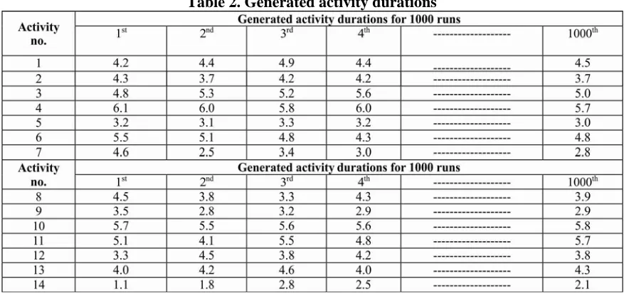
We now consider how the cost parameters in our model derived mathematically can be compared with the performance of an individual customer in simulated system recently given by Mandoza etal [2014]. Through its simulation study and randomly generated numbers studied in three different experiments, 929 scenarios in one experiment, 1440 in second and 337 in third experiment and find out that approximatelyin 93 % instances where

( )

C

α

has two inflection point and minimum occurs at

α

between 0 and 1. In third scenario, he illustrated that ( )

C

α

has one inflection point and minimum occurs at a value of

α

closed to one. When the demand is