An Efficient Heuristic Algorithm for Solving
Connected Vertex Cover Problem in Graph Theory
Yongfei Zhang1, Jun Wu1, Liming Zhang2,3, Peng Zhao1, Junping Zhou1,2,* and Minghao Yin1,2
1 College of Information Science and Technology, Northeast Normal University, Changchun, 130117, China 2 Key Laboratory of Symbolic Computation and Knowledge Engineering of Ministry of Education,
Changchun 130012, China
3 College of Computer Science and Technology, Jilin University Changchun 130012, China
* Correspondence: [email protected]
Version January 25, 2018 submitted to
Abstract: The connected vertex cover (CVC) problem is a variant of the vertex cover problem, 1
which has many important applications, such as wireless network design, routing and wavelength 2
assignment problem, etc. A good algorithm for the problem can help us improve engineering 3
efficiency, cost savings and resources in industrial applications. In this work, we present an efficient 4
algorithm GRASP-CVC (Greedy Randomized Adaptive Search Procedure for Connected Vertex 5
Cover) for CVCin general graphs. The algorithm has two main phases, i.e., construction phase 6
and local search phase. To construct a high quality feasible initial solution, we design a greedy 7
function and a restricted candidate list in the construction phase. The configuration checking strategy 8
is adopted to decrease the cycling problem in the local search phase. The experimental results 9
demonstrate that GRASP-CVC is competitive with the other competitive algorithm, which validate 10
the effectivity and efficiency of our GRASP-CVC solver. 11
Keywords:Heuristic algorithm; connected vertex cover; GRASP. 12
1. Introduction 13
The connected vertex cover(CVC) is one of the classical combinatorial optimization problems, 14
which was first introduced by Garey and Johnson in paper [1]. The problem not only shows its great 15
importance in theory, but also has many significant industrial applications [2–5]. For example, in the 16
wireless newtwork design, the vertices of the newtwork are connected by transmission links. We 17
want to place a minimum number of relay stations on vertices such that any pair of relay stations are 18
connected and every transmission link is incident to a relay station. This is the most direct application 19
of the connected vertex cover model in the industry. Designing a good algorithm to solve this problem 20
can not only improve work efficiency, save money and labor cost, but also save natural resources and 21
reduce material waste. The problem is known to be NP-hard even in the planar 2-connected graph of 22
maximum degree 4 [6], planar bipartite graph with maximum degree 4 [7], as well as in 3-connected 23
graph [8]. 24
TheCVC problem has been studied for a long time, and a lot of efforts have been devoted 25
to it. To date, there are mainly two types of algorithms to solveCVC, i.e., exact algorithms and 26
approximation algorithms. All existing exact algorithms forCVCare mainly FPT (fixed-parameter 27
tractable) algorithms in theory and these theoretical results are obtained in worst case. For example, 28
Moser [2] showed thatCVCis fixed-parameter tractable using the tree width as a parameter and 29
proposed a dynamic programming algorithm running inO(2w·w3w+2·n)time, wherewis the tree
30
width,nis the number of nodes of nice tree decomposition. With the desired vertex cover sizekas 31
parameter, Richter et al. [9] proposed an improved algorithm with running time in O(2.7606k) in the 32
worst case. Binkele-Raible [10] provided a better exact algorithm with running time inO(2.4882k)in the 33
worst case. Because these exact algorithms fail to solve large graphs, a lot of efforts on approximation 34
algorithms have been devoted. In the general graph, Savage [11] proposed the first constant ratio 35
algorithm and proved that the set of internal nodes of any depth-first search tree is a solution of 36
2-approximation forCVC problem. In addition, Fujito and Doi [12] proposed a 2-approximation 37
algorithm for solving CVC, which runs inO(log2n)time usingO(δ2(m+n)/logn)processors on an
38
EREW-PRAM, wheren is the number of vertices,mthe number of edges, andδis the maximum 39
vertex degree. Fernau and Manlove [7] proved thatCVCis NP-hard to approximate within 10√5−21 40
in general graphs unlessP = NP. Therefore, it is difficult to improve the approximation ratio of 41
approximation algorithms in general graphs, which makes the researchers change their research angle 42
into the special graphs. Escoffier et al. [13] proved that theCVCproblem is APX-complete in bipartite 43
graphs of maximum degree 4 and is polynomial time solvable in chordal graphs. In addition, they also 44
showed that CVC is 5/3-approximable for a class of special graphs (where solving the minimum vertex 45
cover problem used polynomial time) and a polynomial time approximation algorithm forCVCin 46
planar graphs was presented. Cardinal and Levy [14] proposed an approximation algorithm in dense 47
graphs and the algorithm approximated theCVCproblem with a ratio strictly less than 2 in dense 48
graphs. The first polynomial time approximation algorithm in unit disk graphs forCVCproblem was 49
proposed in [3]. Li et al.[15] proved that theCVCproblem is still NP-hard for 4-regular graphs and 50
provided a lower bound for the problem. Moreover, they proposed two approximation schemes for this 51
problem in 4-regular graphs with approximation ratio 3/2 and 4/3+O(1/n), respectively. Although 52
the exact algorithms forCVCcan provide an optimal solution, they are hard and time consuming to 53
deal with large scale instances. Furthermore, although some approximation algorithms forCVCcan 54
get good performance in special graphs, they are usually not suitable for dealing with general graphs, 55
and the state-of-the-art approximation methods in general graphs can only provide an approximate 56
ratio 2, which is often not enough in practice. This yields a new challenge for us to devise a heuristic 57
algorithm forCVCthat can deal with large general graphs and obtain the best possible approximate 58
solutions within a reasonable time. 59
In this article, the heuristic algorithm GRASP-CVC forCVCin general graphs is proposed and 60
this algorithm can obtain a relatively good solution within a reasonable time. The heuristic algorithm 61
GRASP-CVC is based on the framework of greedy randomized adaptive search procedure (GRASP) 62
[16]. The algorithm GRASP-CVC has two main phases, i.e., construction phase and local search phase. 63
The GRASP-CVC tries to construct a feasible initial solution greedily in the construction phase. During 64
this phase, we design a greedy function to help to evaluate the benefit of adding a vertex to the 65
current solution. Besides, we construct a restricted candidate list (RCL) to assist in constructing a 66
high quality initial solution in the construction phase. Then the initial solution is further improved 67
in the local search phase. To prevent the local search from suffering severe cycling problem, the 68
configuration checking (CC) strategy is adopted in the search. Relying on theCC, we avoid many 69
unnecessary searches during the local search procedure and the efficiency of the GRASP-CVC is 70
improved greatly. Once the local search phase cannot explore a better solution anymore, which means 71
the local search phase reaches a local optima, the GRASP-CVC then restarts a new iteration and repeats 72
the construction and local search phases until reaching the maximum iteration times. The best found 73
solution will be the final solution after all iterations used up. The results of experiments demonstrate 74
that GRASP-CVC provides better solutions compared to the competitive algorithm, which validate the 75
effectivity and efficiency of our GRASP-CVC solver. Moreover, the GRASP-CVC obtains almost the 76
same size solutions in 10 times running, which demonstrates GRASP-CVC is stable. 77
The rest of this paper is structured as follows. Some relevant definitions and background 78
knowledge will be introduced in next section. In Section 3, the algorithm GRASP-CVC will be 79
introduced and the two main components will be discussed in details. Experimental evaluations and 80
analyses will be shown in Section 4. Conclusions and future work will be given in the last section. 81
2. Preliminaries 82
In this section, some definitions and background knowledge are provided. From now on, unless 83
a
b
c
d
e
g
f
c
e
c
d
e
(a)
(c) (b)
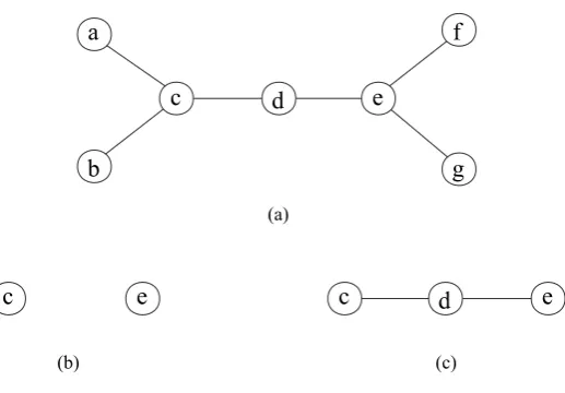
Figure 1.An example for MVC and CVC.
V= {v1,v2, ...,vn}is the vertices set andE={e1,e2, ...,em}is the edges set. In addition, each edge
85
ei= (vk,vj)(16i6m, 16k,j6n,k6=j)is a 2-element tuple onVand we define verticesvkandvj
86
are the endpoints of edgeei. For a vertex subsetC⊆Vand an edgeei, ifCcontains no endpoint ofei,
87
we sayeiis uncovered byC, otherwise, we sayeiis covered byC.
88
Definition 1. (Vertex Cover, VC) Given a graph G= (V,E), a subset of vertices C⊆V is a vertex cover(VC) 89
of G if each edge in E has at least one endpoint in C. 90
Definition 2. (Minimum Vertex Cover, MVC) Given a graph G= (V,E), the minimum vertex cover (MVC) 91
problem is to compute a VC of minimum cardinality in G. 92
Definition 3. (Induced Sub-graph, IS) Given two graph G= (V,E)and G0 = (V0,E0)where V0 ⊆V and 93
E0={(v,u)v,u∈V0∧(v,u)∈E}, G0is called an induced sub-graph (IS) of G. 94
Definition 4. (Connected Graph) A graph is a connected graph if there is a path between every pair of vertices. 95
Definition 5. (Connected Vertex Cover, CVC) Given a connected graph G = (V,E), the connected vertex 96
cover (CVC) problem is to determine a subset C ⊆ V with minimum cardinality such that C satisfies the 97
following two conditions: 1) C is a vertex cover; 2) the IS induced by C is a connected graph. 98
In order to facilitate the readers to understand the concepts given above, we provide an 99
example in Figure 1. Figure 1(a) is a graph G = (V,E), where V = {a,b,c,d,e,f,g} and 100
E={(a,c),(b,c),(c,d),(d,e),(e,f),(e,g)}. Figure 1(b) presents an induced sub-graph by the vertex 101
setV10 ={c,e}, which is just the solution of theMVCproblem ofG. Because the induced sub-graph in 102
Figure 1(b) is not connected, the vertex setV10 ={c,e}is not the solution of theCVCproblem ofG. 103
By adding a vertexdtoV10, we obtain a new vertex setV20 ={c,d,e}. The sub-graph induced byV20 104
is shown in Figure 1(c). From Figure 1(c), we can notice that the vertex setV20is the minimal vertex 105
subset that satisfies: 1) sub-graph induced byV20is connected; 2) the vertex setV20covers all edges inE. 106
Thus,V20is a solution for theCVCproblem ofG. From the example, we see that the size of the optimal 107
MVCsolution provides a lower bound for the size of the optimalCVCsolution. In the following, we 108
will present the conclusion in Theorem 1. 109
Theorem 1. The size of the optimal MVC solution provides a lower bound for the size of the optimal CVC 110
Proof. Given an undirected graphG, we suppose the size of the optimalMVCsolution isNand the 112
size of the optimalCVCsolution isM. Then we will analyze the theorem cases individually. 113
Case 1. There is a connected optimal solution ofMVC. Under this circumstance, theMVCsolution is 114
also aCVCsolution. Thus, we haveM=N. 115
Case 2. There is no connected solution among all of the optimal solutions of MVC. Under this 116
condition, it is impossible thatM = N. Then we will prove the conclusion by using reduction to 117
absurdity. Suppose there exists aCVCsolution thatM6N. Under this condition, according to the 118
definitions ofCVCandMVC, we know theCVCsolution is anMVCsolution as well. So, we get one 119
MVCsolution whose size is less thanN. However, this is contradiction with the previous assumption 120
thatNis the size of the optimalMVCsolution. 121
In total, we finally reach the conclusion thatM>N, which means that the optimalMVCsolution size 122
provides a lower bound for the size of the optimalCVCsolution. 123
3. GRASP-CVC algorithm for CVC 124
GRASP-CVC (Greedy Randomized Adaptive Search Procedures for Connected Vertex Cover 125
problem) is a multi-start meta-heuristic, which consists of two main phases: construction phase 126
and local search phase. An initial solution is constructed firstly in the construction phase, and 127
then the local search phase attempts to find the existence of a better solution by exploring the 128
neighborhood of the initial solution. The two phases are executed repeatedly until reaching the 129
termination condition, and then the GRASP-CVC takes the best found solution as the final output. The 130
pseudo code of GRASP-CVC is outlined in Algorithm 1. At first, the solutionC∗is initialized (line 1). 131
Then the algorithm enters an iteration loop (line 2-8). In each iteration, an initialCVCsolutionCis 132
generated firstly by the construction procedure (line 3), and then in the local search procedure (line 4), 133
GRASP-CVC starts its search fromCtrying to find a better solution. IfCpossesses fewer vertices than 134
the current best solutionC∗,C∗will be updated byC(line 5-6). When the GRASP-CVC reaches the 135
maximum iteration times,C∗will be returned as the final solution (line 9). During the construction, 136
we design a greedy function and construct a restricted candidate list to help to construct a high quality 137
feasible solution. Moreover, in the local search, we adopt the configuration checking to reduce the 138
cycling problem. The two phases will be discussed in details in the next two subsections. 139
140
Algorithm 1:GRASP-CVC(MaxIter,seed)
1 initialize the solutionC∗; 2 fori=1to MaxIterdo
3 C=GreedyConstruction(seed); 4 C= LocalSearch(C);
5 if|C|<|C*|then
6 C∗=C;
7 end
8 end
9 returnC∗
3.1. Construction phase 141
Before introducing the construction phase, we shall give the definitions of greedy function and 142
restricted candidate list (RCL) that play important roles in the construction phase. 143
3.1.1. Greedy function and RCL 145
To evaluate the benefit of addingvto the current solution, a greedy functionscore(v) is designed, which is quite important for the construction ofRCLas well. In order to introduce the greedy function, we firstly propose some relevant definitions. We say verticesuandvare neighbors each other if there is an edge between them, and we useN(u) ={v|(u,v)∈E}denoting the neighbors set of vertexu. The neighbor vertices set of a solutionC, denoted asN(C), can be calculated as follows.
N(C) ={v|v∈/C,v∈N(u),u∈C,N(u) ={v|(u,v)∈E}} (1) For a given vertexv, the greedy functionscore(v) can be calculated by the Formula (2).
score(v) =cost(C)−cost(C0) (2) In the Formula (2),Cis the current solution. IfvinC,C0=C\{v}(’\’ means removing the vertexv fromC), otherwise,C0=C∪ {v}. Moreover,cost(C) is also a function calculated by the Formula (3).
cost(C) =|{e|e is not covered by C}| (3) From the formula, we can know that the functioncost(C) is to compute the total number of edges 146
uncovered byC. In addition, whenvinC,score(v) is a negative number. 147
148
Using the greedy functionscore(v), we can identify those vertices that are most beneficial to the 149
current solution. Moreover, the greedy function is an indispensable part in the construction ofRCL. 150
The RCL consists of the vertices that are most beneficial to the current solution C. In the construction phase, one vertex is chosen randomly from RCL. And to construct a feasible initial solution, we select vertices fromRCL. The construction ofRCLis described in Formula (4)
RCL={v|v∈N(C)∧score(v)>score(u),∀u∈N(C)} (4) Clearly, the elements ofRCLare the vertices set that having the highestscorein the premise of not 151
destroying the connectivity ofC. 152
3.1.2. Construction procedure 153
After the necessary descriptions of greedy function and RCL, we shall discuss the greedy 154
construction procedure in details. The greedy construction procedure GreedyConstruction is outlined 155
in Algorithm 2.
Algorithm 2:GreedyConstruction(seed)
1 C=Φ;
2 RCL={v|v∈V∧score(v)≥score(u),∀u∈V};
3 initialize thescoreof each vertex according to Formula(2); 4 whileC is not a connected vertex coverdo
5 choose a vertexvfromRCLrandomly; 6 C={v} ∪C;
7 updatescoreof each vertex;
8 RCL={v|v∈N(C)∧score(v)>score(u),∀u∈N(C)}; 9 end
10 returnC
156
In the beginning, the connected vertex coverCis initialized (line 1) and thescoreof each vertex is 157
initialized according to the Formula (2) (line 2). TheRCLis initialized to the vertices with the highest 158
loop, a vertexvis chosen from theRCLrandomly and added into the construction solutionC(line 5-6). 160
After the operations of line 5 and 6, thescoreof each vertex is updated according to the Formula (2) 161
(line 7). At the end of the loop, theRCLis updated (line 8). The loop is executed untilCis constructed 162
to be a solution ofCVC, and thenCwill be returned at the end of the construction procedure (line 10). 163
3.2. Local search phase 164
In this subsection, we shall introduce the configuration checking (CC) strategy and discuss the 165
working process of the local search phase in details. 166
3.2.1. Configuration checking strategy 167
Greedy strategy is usually an important part in the local search algorithms. It helps to lift the 168
performance of the local search algorithms on large and hard instances. However, the greedy strategy 169
usually also makes the local search algorithms easier to fall into the cycling problem (which means the 170
algorithm visits the same part of the solution space repeatedly). Up to now, many efficient strategies 171
have been used to handle this problem [17–20]. Configuration checking (CC) [21] strategy is one of 172
those strategies and has been applied to some problems successfully [21–25]. Therefore, we adopt the 173
CCstrategy to avoid the cycling problem in the local search. 174
Before introducing theCC, we shall give the concept of vertex state. The vertex state of a vertexv 175
refers to the fact whethervis located in the current solution. We can use a Boolean value 1 to represent 176
vis in the current solution and 0 to represent is not in. The configuration of a vertexvis the states of 177
all its neighbor vertices, which can be denoted by a n-dimensional Boolean vectorcv(wherenis the
178
number of neighbor vertices ofv). 179
The main idea of theCCstrategy is that a vertexvis forbidden to add back to the current solution 180
if its configuration keeps unchanged since it was removed from the current solution last time. This 181
strategy is intuitive and reasonable in avoiding cycling problem, as it prevents the search facing the 182
same scenario again. For example, for av ∈ C, suppose its configuration iscv0 = (0, 1, 0, 1)after
183
removingvout ofC, then after several steps of searching,vis selected again according to the greedy 184
function value and suppose its configuration iscv1now. Ifcv0=cv1,i.e. configuration not changed, if
185
addvback to theC, then the search goes back to the same situation before last time removingvout 186
ofCand the same solution space will be searched repeatedly. However, this situation will not occur 187
whencv06=cv1, i.e. configuration changed(e.g.cv1= (1, 1, 0, 1)). A Boolean arrayChangeis used to
188
implement theCCstrategy. The element in the arrayChangeisChange[v], which denotes whether the 189
configuration of vertexvis changed since it was removed from the current solution last time. We use 190
Change[v] = 1 expressing change, andChange[v] = 0 expressing no change. Only the vertexvwhose 191
Change[v] = 1 is allowed to be added to the current solution in the local search process. In the process 192
of local search, the values ofChangeare updated according the rules below [21]. 193
• Rule 1: In the beginning, for each vertexv, setChange[v] to 1. 194
• Rule 2: When removingvfromC, resetChange[v] to 0. 195
• Rule 3: Whenuchanges its state, for eachv∈N(u)\C,Change[v] is set to 1. 196
3.2.2. Local search procedure 197
In this subsection, the local search procedure is discussed at length. The main steps of the 198
LocalSearch are listed in Algorithm 3. 199
200
The local search procedure performs as follows. In the first place, all elements of theChangeare 201
initialized to 1 (line 1), which means that all vertices are allowed to be added to the current solution 202
in the beginning. Next, the local optimal solutionC∗is initialized asC, whereCis generated by the 203
construction phase (line 2). Then, in the loop (line 3-17), the LocalSearch(C) checks the feasibility of the 204
current solutionC. IfCis aCVCsolution which has a smaller vertex number thanC∗, thenC∗will be 205
Algorithm 3:LocalSearch(C)
1 initialize each element value ofChangearray to 1; 2 C∗=C;
3 whiletruedo
4 ifC is a vertex coverthen 5 ifC is connectedthen
6 if|C|<|C∗|then
7 C∗=C;
8 end
9 else
10 returnC∗;
11 end
12 drop a vertexuwith the highest score fromCand update theChangearray; 13 continue;
14 end
15 choose an uncovered edgeerandomly;
16 choose a vertexv∈esuch thatChange[v] =1 with a higher score,C={v} ∪Cand
update theChangearray;
17 end
starts the next cycle (line 4-14). IfCis aVCbut not aCVCanymore aftervis removed, which means 207
the procedure reaches a local optimal solution, thenC∗will be returned as the final result of the local 208
search procedure (line 9-11). IfCis not aVCanymore aftervis removed, the procedure chooses an 209
uncovered edgeerandomly, then chooses a vertexv ∈esuch thatChange[v]=1 with a higherscore, 210
and adds toC ={v} ∪C(line 15-16). TheChangearray is updated according to Rule 2 and Rule 3 211
when a vertex changes its state (line 12,16). 212
3.3. Time complexity analysis 213
In this subsection, we discuss the time complexity of the main components of the GRASP-CVC 214
algorithm. 215
First, we consider the algorithm for constructing the initial solution. In each loop, we need 216
to update thescorefor |V|vertices, and scan|N(C)|vertices in order to update theRCL. If every 217
time we add a vertex to C, an average of d edges are covered. Then, we can get a solution in 218
O(|E|/d∗(|V|+|N(C)|)) =O(|E| ∗ |V|). 219
Next, we consider the time complexity of the local search algorithm. In this part, there are three 220
operations that affect the running time of the algorithm:drop a vertex from C(Algorithm 3, line 12), 221
choose an uncovered edge(Algorithm 3, line 15), andupdate the Change array(Algorithm 3, line 12 and 222
16). Since the number of vertex inCis|C|, the first operation can be done in a time ofO(|C|). In our 223
implementation, we maintain a set to record uncovered edges, so an uncovered edge can be chosen in 224
O(1). The time complexity of the third operation depends on the degree of the operated vertex, and 225
therefore this work can be done in O(δ), whereδis the maximum degree of the vertices. Thus, the time 226
complexity of the local search isO(|C|+1+δ) =O(|C|+δ). 227
Overall, the run-time complexity of the GRASP-CVC isO(|E| ∗ |V|+|C|+δ). 228
229
4. Computational experiments 230
During this section, the effectivity and efficiency of the GRASP-CVC algorithm are evaluated 231
by performing some comparison experiments. We compare the GRASP-CVC algorithm with the 232
currently best approximate algorithm (2-approximation algorithm) we know in general graphs [12]. 233
approximationCVCsolver, so we implement the 2-approximation algorithm proposed in [12]. We 235
implement the algorithms GRASP-CVC, and the 2-approximation algorithm in the C++ programming 236
language. All of the experiments are carried on a work station under windows 7 operating system, 237
3.30GHZ CPU and 8GB memory. 238
4.1. Benchmark instances 239
In the experiments, we choose two well-known benchmarks in the field ofMVCresearch, the 240
DIMACS and BHOSLIB instance sets. DIMACS benchmark contains both structured and randomized 241
instances. The structured instances are generated from practical problems, such as coding theory, 242
Keller conjecture and so on. The randomized instances are generated from the stochastic models, such 243
as brock instances. The scale of these problem instances is from 50 vertices and 1000 edges to more than 244
5500 vertices and 5 million edges. BHOSLIB benchmark is famous for its hardness. The benchmark 245
instances are transformed fromSATinstances that are generated in the phase transition area. And the 246
instances in the phase transition area have been proved hard. From the two benchmarks, we select 37 247
DIMACS benchmark instances and 40 BHOSLIB benchmark instances, which are all employed in the 248
bestMVCsolver [25]. 249
4.2. Experiment parameter settings 250
Before reporting the experimental results, we shall introduce some parameter settings. 251
In GRASP-CVC, there are two main parameters: maximum number of iterations (MaxIter) and 252
random seed (seed). According to our experimental experience, we setMaxIterto 5000 and random 253
seed to an interval from 1 to 10. In order to evaluate the robustness of GRASP-CVC, we execute ten 254
times for each instance using different random seeds. 255
For the sake of comparison between GRASP-CVC and 2-approximation algorithm for CVC, 256
we execute ten times independent runs for the approximation algorithm as well. In addition, 257
since the 2-approximation algorithm runs very fast, there is no need to set the cut-off time for the 258
2-approximation algorithm, we just set the cut-off time for GRASP-CVC to 1000 seconds. 259
4.3. Experimental results 260
In this subsection, we will provide the computational results of GRASP-CVC (GRASP-CVC) and 261
the 2-approximation algorithm (2-Aprox) on the two chosen benchmarks. In the results, we provide 262
the following information: the number of vertices and edges of each instance (|V|,|E|), the best known 263
size of theMVCsolution (MVC), the best solution size solved by the corresponding algorithms (best), 264
the average size of solutions solved by the corresponding algorithms (avg), the average time consumed 265
by the corresponding algorithms (time). In addition, theMVCsize with star (*) has been proved to be 266
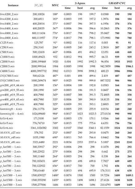
Table 1.Experimental result on DIMACS Instances
Instance |V|,|E| MVC 2-Aprox GRASP-CVC
time best avg time best avg
brock200_2.mis 200,10024 188* 0.0003 198 199.7 0.0388 190 190
brock200_4.mis 200,6811 183* 0.0003 195 197.2 1.3976 184 184
brock400_2.mis 400,20014 371* 0.0007 396 397.5 6.1956 376 376
brock400_4.mis 400,20035 367* 0.0006 396 396.6 10.2863 376 376
brock800_2.mis 800,111434 776* 0.0017 798 798.2 35.0407 780 780
brock800_4.mis 800,111957 774* 0.0017 798 798.1 173.9981 780 780
C125.9.mis 125,787 91* 0.0002 116 117.4 0.003 91 91
C250.9.mis 250,3141 206* 0.0005 240 243.2 2.3818 207 207
C500.9.mis 500,12418 443* 0.0006 491 494.2 12.051 448 448
C1000.9.mis 1000,49421 932 0.0012 994 995.7 66.33 939 939
C2000.9.mis 2000,199468 1920 0.004 1992 1992.3 96.854 1933 1933
C2000.5.mis 2000,999164 1984 0.0085 1998 1998 942.5859 1986 1986.1
C4000.5.mis 4000,3997732 3982 0.0313 3998 3998.2 400.23 3986 3986
DSJC500.5.mis 500,62126 487* 0.001 498 499.6 2.419 487 487
DSJC1000.5.mis 1000,249674 985* 0.0025 998 999.8 887.5232 986 986
gen200_p0.9_44.mis 200,1990 156* 0.0004 189 192.8 0.0583 164 164
gen200_p0.9_55.mis 200,1990 145* 0.0003 186 191.5 0.0607 156 156
gen400_p0.9_55.mis 400,7980 345* 0.0007 388 391.5 72.4805 358 358
gen400_p0.9_65.mis 400,7980 335* 0.0006 389 390.9 18.8135 354 354
gen400_p0.9_75.mis 400,7980 325* 0.0009 391 393.1 2.8003 357 357
hamming8−4.mis 256,11776 240* 0.0005 255 255.9 0.0154 240 240
hamming10−4.mis 1024,89600 984* 0.0017 1023 1023.5 273.0134 990 990
keller4.mis 171,5100 160* 0.0003 170 170.1 3.9266 160 160
keller5.mis 776,74710 749* 0.0015 775 775.6 4.6351 756 756
keller6.mis 3361,1026582 3302 0.0107 3360 3360.1 82.1559 3324 3324
MANN_a27.mis 378,702 252* 0.0007 290 293.8 0.0475 260 260
MANN_a45.mis 1035,1980 690* 0.0011 765 766.4 0.8462 704 704
MANN_a81.mis 3321,6480 2221 0.0034 2353 2357.6 5.1007 2241 2241
p_hat300−1.mis 300,33917 292* 0.0006 298 298 0.1078 292 292
p_hat300−2.mis 300,22922 275* 0.0004 298 298 0.642 275 275
p_hat300−3.mis 300,11460 264* 0.0003 294 296 0.338 264 264
p_hat700−1.mis 700,183651 689* 0.0019 698 699.8 7.7827 689 689
p_hat700−2.mis 700,122922 656* 0.0017 700 700 1.792 656 656
p_hat700−3.mis 700,61640 638* 0.0013 694 695.9 176.3111 638 638
p_hat1500−1.mis 1500,839327 1488* 0.0074 1500 1500 19.7254 1489 1489.1
p_hat1500−2.mis 1500,555290 1435* 0.0051 1498 1498.1 27.6126 1438 1438
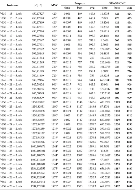
Table 2.Experimental result on BHOSLIB Instances
Instance |V|,|E| MVC 2-Aprox GRASP-CVC
time best avg time best avg
f rb30−15−1.mis 450,17827 420* 0.001 449 449.6 11.3735 424 424
f rb30−15−2.mis 450,17874 420* 0.0006 447 448.4 7.873 425 425
f rb30−15−3.mis 450,17809 420* 0.0007 449 449.7 13.4266 424 424
f rb30−15−4.mis 450,17831 420* 0.0006 448 449.3 15.2355 424 424
f rb30−15−5.mis 450,17794 420* 0.0005 448 449.3 25.6118 423 423
f rb35−17−1.mis 595,27856 560* 0.0011 592 593.7 29.4486 565 565
f rb35−17−2.mis 595,27847 560* 0.0009 592 592.8 8.5406 565 565
f rb35−17−3.mis 595,27931 560* 0.001 592 592.7 2.7005 565 565
f rb35−17−4.mis 595,27842 560* 0.001 592 593.6 172.9833 565 565
f rb35−17−5.mis 595,28143 560* 0.0009 594 594.5 34.4835 565 565
f rb40−19−1.mis 760,41314 720* 0.0012 758 759 187.7404 728 728
f rb40−19−2.mis 760,41263 720* 0.0012 757 758 213.6616 726 726
f rb40−19−3.mis 760,41095 720* 0.0012 758 759.2 101.0795 725 725
f rb40−19−4.mis 760,41605 720* 0.0012 757 758.1 8.3877 726 726
f rb40−19−5.mis 760,41619 720* 0.0014 758 759 33.3235 725 725
f rb45−21−1.mis 945,59186 900* 0.0015 944 944.4 665.5343 908 908
f rb45−21−2.mis 945,58624 900* 0.0017 942 943.3 83.904 908 908
f rb45−21−3.mis 945,58245 900* 0.0015 941 943 479.1447 908 908
f rb45−21−4.mis 945,58549 900* 0.0019 941 942.6 135.2191 907 907
f rb45−21−5.mis 945,58579 900* 0.0019 943 943.7 235.1495 909 909
f rb50−23−1.mis 1150,80072 1100* 0.0016 1146 1147.6 409.0972 1109 1109
f rb50−23−2.mis 1150,80851 1100* 0.0018 1147 1148.6 87.4731 1110 1110
f rb50−23−3.mis 1150,81068 1100* 0.0021 1147 1148.1 414.1894 1110 1110
f rb50−23−4.mis 1150,80258 1100* 0.002 1147 1148.5 431.3235 1110 1110
f rb50−23−5.mis 1150,80035 1100* 0.002 1147 1148.3 837.1014 1109 1109
f rb53−24−1.mis 1272,94227 1219* 0.002 1269 1270.7 695.5386 1230 1230
f rb53−24−2.mis 1272,94289 1219* 0.0022 1269 1270.4 390.4401 1230 1230
f rb53−24−3.mis 1272,94127 1219* 0.002 1270 1271.2 552.5761 1229 1229
f rb53−24−4.mis 1272,94308 1219* 0.0024 1270 1270.4 588.6573 1229 1229
f rb53−24−5.mis 1272,94226 1219* 0.0022 1270 1270.6 95.6667 1230 1230
f rb56−25−1.mis 1400,109676 1344* 0.0022 1398 1399.1 90.5451 1357 1357
f rb56−25−2.mis 1400,109401 1344* 0.0022 1397 1397.3 412.38 1353 1353
f rb56−25−3.mis 1400,109379 1344* 0.0023 1397 1398.6 190.6417 1356 1356
f rb56−25−4.mis 1400,110038 1344* 0.0025 1398 1399 47.1687 1356 1356
f rb56−25−5.mis 1400,109601 1344* 0.0023 1397 1398.4 616.9286 1355 1355
f rb59−26−1.mis 1534,126555 1475* 0.0027 1533 1533.2 656.1494 1487 1487
f rb59−26−2.mis 1534,126163 1475* 0.0024 1531 1532.5 100.0605 1488 1488
f rb59−26−3.mis 1534,126082 1475* 0.0026 1531 1532.5 495.5281 1489 1489
f rb59−26−4.mis 1534,127011 1475* 0.0027 1531 1532.4 319.4073 1487 1487
In Table 1, we present the experimental results on DIMACS benchmark. As is shown in the 268
table, compared to the 2-Aprox algorithm, GRASP-CVC finds the better qualityCVCsolutions on 269
all the 37 DIMACS instances. On most instances, the solutions found by GRASP-CVC are very close 270
to the optimalMVCand it even finds the same size solutions as optimalMVCon 10 instances in a 271
very short time, which means it finds the optimalCVCsolutions on these 10 instances. Besides, the 272
GRASP-CVC consumes very little time on most of the instances, which indicates the efficiency of the 273
GRASP-CVC. Moreover, the GRASP-CVC takes a relatively long time on several larger instances (such 274
asC2000.5.mis,DSJC1000.5.mis,C4000.5.misand so on), this shows that the algorithm still has room for 275
improvement. Another point worth noting is that though the 2-Aprox takes the less time on all of the 276
37 instances, most of its solutions are not so satisfactory compared to GRASP-CVC. 277
Table 2 provides the results on BHOSLIB benchmark. We can get the same conclusion as DIMACS 278
that the GRASP-CVC performs best, even though it takes much more time than 2-Aprox. The solutions 279
found by GRASP-CVC are close to the optimalMVC, which means the GRASP-CVC is very effective. 280
The columnsbestandavgof GRASP-CVC have the same values on almost all of the instances, which 281
means that the GRASP-CVC gets almost the same size solutions in ten times runs and this demonstrates 282
the stability of the GRASP-CVC. 283
The comparison and experimental analyses above show that the GRASP-CVC has very good 284
effectivity and efficiency forCVC problem. It performs better than the competitive algorithm in 285
solution quality. Moreover, the GRASP-CVC gets almost the same size solutions in ten times runs, 286
which demonstrates the stability of the GRASP-CVC. 287
5. Conclusion 288
In this paper, a heuristic algorithm GRASP-CVC for connected vertex cover problem was proposed. 289
A greedy function and a restricted candidate list (RCL) were proposed to help to construct a high 290
quality initial solution. Furthermore, the configuration checking (CC) strategy was employed to reduce 291
the cycling problem and improve the efficiency of the search. Experimental results demonstrate that 292
GRASP-CVC works better than the comparison algorithm, which validates the effectiveness and 293
efficiency of our GRASP-CVC solver. In the future, we will further study various heuristic methods 294
and hope to design a more powerful heuristic algorithm to deal withCVC. 295
Acknowledgments:This work was fully supported by the National Natural Science Foundation of China under 296
Grant No.61370156, No. 61403076, and No. 61403077; Research Fund for the Doctoral Program of Higher 297
Education No. 20120043120017; Program for New Century Excellent Talents in University No. NCET-13-0724; 298
the Large-scale Scientific Instrument and Equipment Sharing Project of Jilin Province (20150623024TC-03);The 299
Natural Science Foundation for Youths of JiLin Province (20160520104JH). 300
References 301
1. Garey, M. R., Johnson, D. S. The rectilinear Steiner tree problem is NP-complete. SIAM Journal on Applied 302
Mathematics,1997, 32(4), 826-834. 303
2. Moser, H. Exact algorithms for generalizations of vertex cover. Master’s thesis, Fakultät für Mathematik und 304
Informatik, Friedrich-Schiller-Universität Jena,2005. 305
3. Zhang, Z., Gao, X., Wu, W. PTAS for connected vertex cover in unit disk graphs. Theoretical Computer 306
Science, 2009, 410(52), 5398-5402. 307
4. Guo, P., Wang, J., Geng, X. H., Kim, C. S., Kim, J. U. A variable threshold-value authentication architecture 308
for wireless mesh networks. Journal of Internet Technology, 2014, 15(6), 929-935. 309
5. Shen, J., Tan, H. W., Wang, J., Wang, J. W., Lee, S. Y. A novel routing protocol providing good transmission 310
reliability in underwater sensor networks. Journal of Internet Technology, 2015, 16(1), 171-178. 311
6. Priyadarsini, P. L. K., Hemalatha, T. Connected vertex cover in 2-connected planar graph with maximum 312
degree 4 is NP-complete. International Journal of Mathematical, Physical and Engineering Sciences, 2008, 313
2(1), 51-54. 314
7. Fernau, H., Manlove, D. F. Vertex and edge covers with clustering properties: Complexity and algorithms. 315
8. Watanabe, T., Kajita, S., Onaga, K. Vertex covers and connected vertex covers in 3-connected graphs. IEEE 317
International Sympoisum on Circuits and Systems. IEEE, 1991, vol.2, 1017-1020. 318
9. Mölle, D., Richter, S., Rossmanith, P. Enumerate and expand: Improved algorithms for connected vertex 319
cover and tree cover. Theory of Computing Systems, 2008, 43(2), 234-253. 320
10. Binkele-Raible, D. Amortized analysis of exponential time-and parameterized algorithms: Measure & 321
Conquer and Reference Search Trees. Praca doktorska, University of Trier, Trier, Germany,2010. 322
11. Savage, C. Depth-first search and the vertex cover problem. Information Processing Letters, 1982, 14(5), 323
233-235. 324
12. Fujito, T., Doi, T. A 2-approximation NC algorithm for connected vertex cover and tree cover. Information 325
processing letters, 2004, 90(2), 59-63. 326
13. Escoffier, B., Gourvès, L., Monnot, J. Complexity and approximation results for the connected vertex cover 327
problem in graphs and hypergraphs. Journal of Discrete Algorithms, 2010, 8(1), 36-49. 328
14. Cardinal, J., Levy, E. Connected vertex covers in dense graphs. Lecture Notes in Computer Science, 2008, 329
5171, 35-48. 330
15. Li, Y., Yang, Z., Wang, W. Complexity and algorithms for the connected vertex cover problem in 4-regular 331
graphs. Applied Mathematics and Computation,2017, 301, 107-114. 332
16. Resende, M. G., Ribeiro, C. C. GRASP: Greedy randomized adaptive search procedures. In Search 333
methodologies, 2014, pp. 287-312, Springer US. 334
17. Zhou, Y., Zhang, H., Li, R., Wang, J. Two local search algorithms for partition vertex cover problem. Journal 335
of Computational and Theoretical Nanoscience, 2016, 13(1), 743-751. 336
18. Li, X., Zhang, J., Yin, M. Animal migration optimization: an optimization algorithm inspired by animal 337
migration behavior. Neural Computing and Applications, 2014, 24(7-8), 1867-1877. 338
19. Wang, Y., Cai, S., Yin, M. Two Efficient Local Search Algorithms for Maximum Weight Clique Problem. In 339
AAAI,2016, pp.805-811. 340
20. Wang, Y.,Yin, M., Ouyang, D., Zhang, L. A novel local search algorithm with configuration checking and 341
scoring mechanism for the set k-covering problem. International Transactions in Operation Research, 2017, 342
24(26),1436-1485. 343
21. Cai, S., Su, K., Sattar, A. Local search with edge weighting and configuration checking heuristics for minimum 344
vertex cover. Artificial Intelligence, 2011, 175(9-10), 1672-1696. 345
22. Luo, C., Cai, S., Wu, W., Su, K. Double Configuration Checking in Stochastic Local Search for Satisfiability. 346
In AAAI, 2014,pp.2703-2709. 347
23. Luo, C., Cai, S., Wu, W., Jie, Z., Su, K. CCLS: an efficient local search algorithm for weighted maximum 348
satisfiability. IEEE Transactions on Computers, 2015, 64(7), 1830-1843. 349
24. Gao, J., Wang, J., Yin, M. Experimental analyses on phase transitions in compiling satisfiability problems. 350
Science China Information Sciences, 2015, 58(3), 1-11. 351
25. Cai, S., Su, K., Luo, C., Sattar, A. NuMVC: An efficient local search algorithm for minimum vertex cover. 352