Designing an experimental rig for developing a fire severity model using numerical simulation

Designing an experimental rig for developing a fire severity model using

numerical simulation

Khalid A. M. Moinuddin, Trong Dac Nguyen and HM Iqbal Mahmud

Centre for Environmental Safety and Risk Engineering, Victoria University P.O. Box 14428, Melbourne, Victoria 8001, Australia

ABSTRACT

In this study, an experimental rig representing a deep enclosure was designed to be used to validate a CFD-based fire model in predicting the outcome. The model then can be used for further study to investigate physical phenomenon within a deep enclosure and to develop an engineering fire severity (heat release rate, HRR, vs time vs position [1]) model. Two empirical models (the VU model [1] and Kawagoe model [2]) were used along with Fire Dynamics Simulator (FDS) in designing the experimental rig. For a specific sized enclosure, when the HRR was prescribed to the FDS as input from the VU model, it was accurately re-produced, while the HRR from the Kawagoe was used as the input the FDS calculated much lower value. The experimental rig of that specific size was then built and various parameters were measured from the tests with liquid fuel fire within this experimental rig. The measured HRR was prescribed into the FDS and the FDS could reproduce HRR values well. However, the predicted temperature and radiation flux was not as good, especially when the flames were near the opening. This may be due to the tendency of flames over-projecting outside the opening in FDS simulations.

Keywords: heat release rate, deep enclosure, CFD-based fire model, fire severity model,

1 INTRODUCTION

Understanding the behaviour of fire in an enclosure, its effect on structure and the safety of occupants in a building is imperative in designing an efficient strategy of safety for the fire engineers. The development of a fire in an enclosure of a building not only depends on the quantity of the combustible/flammable material and the location of the ignition point in the enclosure, but also strongly governed by the geometry of the enclosure. In addition, the variety of the combustible/flammable materials as well as the size and shape of the enclosure can critically affect the behaviour of fire in the enclosures and can turn it to be more challenging in designing the safety plan

NOMENCLATURE

Ao ventilation area (m2)

At total inside surface area of the enclosure (m2)

D depth of enclosure (m) h height of opening (m)

Hc heat of combustion of the fuel (MJ/kg) H height of enclosure (m)

HRR, Q. rate of heat release (kW) HRRPUA, rate of heat release per unit area

a

m

.

rate of air inflow into a fully developed fire (kg/s)

tb burnout time (sec) W width of enclosure (m) w width of opening (m)

Greek symbols

ℛ predicted values

𝜓𝜓 reference values

𝜉𝜉 difference between predicted and reference value

Subscripts

air air

avg average

g gas

i number, i= 1, 2… n

m mean

Figure 1: Typical layout of a deep enclosure (after Moinuddin and Thomas [1])

A series of small-scale experiments with various enclosure sizes, locations of fire and geometries of opening were carried out in the study of Beji et al. [6]. This study measured the HRR and combustion gases under a calorimeter hood as well as the temperature inside the enclosure using thermocouple trees at various locations. It is noted that the inflow rate of air and HRR was only affected by the shape of opening but not the length of the enclosure. It was also reported that the vertical distribution of gas temperatures inside the enclosure was nearly uniform with that for height when ventilation-controlled conditions were established.

One of the benchmark experimental works was conducted by Moinuddin and Thomas [1], who investigated the behaviour of fires in deep enclosures. They reported that the fire duration in a deep enclosure was significantly affected by the height of the opening. With the same width of opening, the fire duration doubles if the height of opening reduces to the half the size. Their work also showed that the burning rate was dropped to about 50% when the opening height was reduced to half without changing the width of the enclosure. Their work [1] proposed a model named the VU model, which can be used for the calculation of the HRR based on the enclosure geometry. They also compared the results of the VU model with that of the Conseil International du Batiment (CIB) model [1, 7] and the Society of Fire Protection Engineers (SFPE) model [1, 8-9] using experiments carried out with different compartment opening sizes. The results indicate that, for deep enclosures, where D/H ≥ 2 and D/W ≥ 2, the VU model shows better performance, while in deep but square compartments (D/H ≥2 and D/W<2), the CIB model or the SFPE method should be used.

It is important that models for the calculation of the HRR based on the enclosure geometry be verified in full-scale configuration. The establishment of a full-scale test for observing fire behaviour in deep enclosures is very expensive and takes a long time. Therefore, consideration should be given to using scaling relationships [3] or a Computational Fire Dynamic (CFD) model as alternative methods to predict fire behaviour in deep enclosures. However, it is essential to design a scaled experimental rig that can be used in predicting full-scale fire behaviour and/or the validation of the CFD simulations with predictive capability of fire development in the deep enclosure.

Thomas et al. [10] performed a numerical study using a CFD based model, Fire Dynamic Simulator, version 4 (FDS4), and compared the results with the experimental data by Moinuddin and Thomas [1]. The results show that the initial movement of the flame-front through the enclosure in FDS4 was similar to that found experimentally. However, the predicted timing of movement of the flame-front later in the fire, and predicted HRR and gas and steel wall temperatures vary greatly from the experimental values. Finally, Thomas et al. [10] concluded that FDS4 could not simulate experiments in deep enclosures measuring 8m x 2m x 0.6m. Therefore, FDS must be improved and/or the experimental rig redesigned (as the depth, D to height, H ratio of D/H=13 which is apparently too high).

Recently, a new version of FDS (version 6) [11] has been released with improved evaporation and combustion sub-models. Therefore this study aims to redesign the experimental rig in which fire behaviour can be accurately simulated using FDS6. Once the FDS model is validated against the experimental results, the behaviour of fires in the deep enclosure can be understood evidently and this can be utilized to develop an appropriate fire severity model for deep enclosures.

However, in this study the validation is limited to prescribed HRR [12] only. In this approach, when the fire size is prescribed in HRR, FDS calculates volatile (gaseous form of the fuel) production rate (mass loss rate of the fuel) by dividing the prescribed fire size by heat of combustion (Hc) of the fuel. The fuel bed created in FDS then acts as a pump which pumps volatiles

combustion model and HRR is re-calculated (in other word the prescribed HRR is readjusted based on oxygen availability) and the resulting transport of heat and combustion products is also simulated. It is aimed to see firstly, whether the combustion model can reproduce the prescribed HRR which is obtained from experiment with the same oxygen availability and secondly, with reasonable reproduction of the HRR, how well FDS can calculate solid surface temperature, flame temperature and radiation flux.

2 RIG DESIGNING TECHNIQUE

2.1 Concept of rig design

The concept of rig designing is a trial and error method. The steps are given below:

Step 1: Nomination of size and shape of a “pure” deep enclosure, where D/H ≥ 2 and D/W ≥ 2 or for one which is deep but square enclosures (D/H ≥2 and D/W<2) [1].

Step 2: Calculation of HRR using empirical models, such as the Kawagoe equation [2] and the VU model [1].

Step 3: Prescription of this calculated HRR into FDS6 to examine the recalculation of HRR by FDS as discussed above.

Step 4: If the prescribed and FDS calculated HRRs are not the same, changing the enclosure dimensions (step 1) and repeating redo steps 2 and 3. This process is continued until the prescribed and the predicted HRRs are nominally same.

2.2 Detailed Technique

In this study, based on [10], the depth of the experimental rig is considered to reduce so that the depth to height ratio is halved from D/H=13. Therefore the depth was set as 4m. As the variation of many parameters can be too complex, the width of the rig is fixed as 2m thereby D/W ≥ 2 condition is fulfilled. The parameter height (H) is needed to vary by maintaining D/H ≥ 2 condition. Three different heights are chosen: 0.6m (D/H~6.67), 0.8m (D/H=5) and 1.0m (D/H=4) to determine an appropriate height to obtain reproducible HRR data from FDS simulation, when the HRR is prescribed.

The FDS6 simulations were conducted for a fire in a deep enclosure with a depth of 4 m, width of 2 m, and for three different heights of 0.6 m, 0.8 m and 1.0 m with the input HRR from the Kawagoe equation and the VU model. After the completion of the simulation, the output HRR, was examined and used to compare with the results from the Kawagoe equation and the VU model. Based on the comparison of the output HRR from FDS and the input HRR obtained from the Kawagoe equation and the VU model, the decision of modifying the experimental rig were made for the next step to carry out the experiments.

2.3 Empirical Models

The Kawagoe Equation

The Kawagoe model was developed by Kawagoe [2] based on a series of experimental tests conducted in the 1950s with full scale rooms as well as model rooms of various constructions. Kawagoe proposed a relationship between the pyrolysis rate and the ventilation through an opening. He showed that the pyrolysis rate not only depends on the ventilation area but also on the height of the ventilation opening [13].

From those tests, Kawagoe identified a new term, named the ‘ventilation factor’ 𝐴𝐴_𝑜𝑜√ℎ, where Ao is

the ventilation area and h is the height of the opening. Based on the ventilation factor, the rate of air inflow (ma) into a fully developed fire in an enclosure is identified as follows [14]:

h

A

m

0

.

5

.

=

.

Q) is calculated as follows:

a air c

m

H

Q

.

=

where

H

h A

Q 1500. o

.

= (kW) ……. (3)

This is the Kawagoe equation which is used to calculate the input HRR for the CFD simulations. The VU Model

Traditionally, the average HRR of a fire in an enclosure is calculated based on the ventilation factor, 𝐴𝐴_𝑜𝑜√ℎ, or its derivative form A₀ h/A_t (with At =total inside surface area of the enclosure),

which consider primarily the shape and size of the opening [1]. However, the dimensions of the enclosure also have effect on the HRR. Therefore a new model was proposed in their study to obtain the HRR based on all of the geometrical parameters of the enclosure with equal emphasis on each parameter. Based on the analysis of various series of experimental results, they developed a model, named as the VU model, for predicting the HRR. The equation of the model is as follows,

HRRavg=1.161×W0.726×D−0.516×H0.766×w0.521×h1.071 ……..(4)

where, w and h are the width and height of the opening, respectively. They emphasized that this model is ideal for applying in deep enclosures (where D/H ≥ 2 and D/W ≥ 2) and it can also work quite well for enclosures where D/H ≥ 2 and D/W = 1 after comparison with the experimental results from CIB tests [15] by eight laboratories in several countries.

For all methods, the duration of the fire or burnout time can be calculated using the following equation [1]:

tb =

(

)

HRR H x (kg) fuel of amount Load Fuel _c

(sec) ………. (5)

2.4 CFD based fire model

Technology (NIST). FDS goes along with Smokeview, a post-processing software tool which is used to observe the fire behaviour, smoke movement and other simulation data calculated from FDS. FDS uses a form of Navier-Stokes equations to study low speed, thermally-driven flow with an emphasis on smoke and heat transport from fires [12].

Two principal methods of simulating fires using FDS are: simulated fire growth and prescribed fire size. In prescribed fire size approach– a fire size is prescribed, usually as a vent with a HRR per unit area (HRRPUA) is specified (which can be varied with time using a ramp function) with specified combustion parameters (including Hc). All other surfaces are specified as

non-combustible. The rest is discussed in Section 1. In simulated fire growth approach, FDS calculates volatiles (gas phase fuel) production rate through simulation of pyrolysis (for solid fuel) or evaporation (for liquid fuel) process. In this study, only the prescribed fire size method is used.

Figure 2. Computational domain with different fuel tray locations in the FDS

Table 1 Thermo-physical, pyrolysis and combustion parameters for CFD based fire modelling

Property Ethanol Steel (from [16])

Thermal conductivity (w/m.k)

T= 20., f=0.168 / T=225., f=0.2 /

T= 20, f=50. / T=677, f=30.6 / Specific heat (kj/kg.k)

T= 20., f=1.1 / T=60., f=1.23 / T=225., f=1.7/

T= 20., f=0.46/ T=377., f=0.60/ T=677., f=0.91/

Density (kg/m3) 790 7850

Heat of combustion (kJ/kg) 25930

Soot yield 0.001

3 IMPLEMENTION OF RIG DESIGNING TECHNIQUE

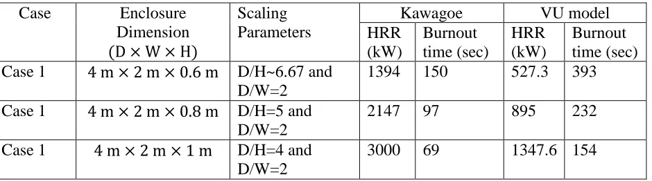
Two trays of fuel measuring 0.9 m × 0.9 m × 0.5 m in size were considered inside the enclosure. Each fuel tray was considered to be filled with 4 kg of ethanol. Based on two empirical models, as discussed in section 2.3, the HRR and burnout times were calculated for dimension of each enclosure and presented in Table 2.

Table 2. Calculated HRR and burnout times by empirical models for dimension of each enclosure

Case Enclosure

Dimension

(D × W × H)

Scaling Parameters

Kawagoe VU model

HRR (kW) Burnout time (sec) HRR (kW) Burnout time (sec) Case 1 4 m × 2 m × 0.6 m D/H~6.67 and

D/W=2

1394 150 527.3 393 Case 1 4 m × 2 m × 0.8 m D/H=5 and

D/W=2

2147 97 895 232

Case 1 4 m × 2 m × 1 m D/H=4 and D/W=2

3000 69 1347.6 154

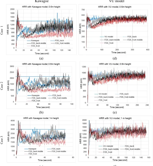
Kawagoe VU model

Ca

se

1

(a) (d)

Ca

se

2

(b) (e)

Ca

se

3

(c) (f)

Figure 3. Comparison of HRR vs time from FDS and empirical models.

(a) After 20 secs (b) After 40 sec

Figure 4 (a) mass fraction of the unburnt gaseous fuel ejected from the vent are filling up behind the flame front via recirculation and (b) larger space is filled up by gas with high mass fraction

ethanol pushing the flame front towards the opening.

4 EXPERIMENTAL PROCEDURE

4.1 Rebuilding the rig

A deep enclosure was built in the Victoria University facility on the Werribee Campus by Moinuddin and Thomas [1] and was used in their works. The enclosure was 8.0m long, 2.0m wide and 0.6m high (D/W of 4 and D/H of ∼13) and it was built by using 1.3mm thick sheet steel.

To establish the experimental setup of this research, the original rig was modified by cutting it in half of the depth. Given that it was built with 1.3 mm thick sheet steel, it is very hard to modify the geometry of the rig. This work could only be done by using both an oxyacetylene welding cutter and triangle grinder. After the original rig was cut, the surface at the side of the cutting was very sharp and had to be filed to make it flat.

Figure 5. The experimental rig after modification of the original enclosure (window locations included)

There were eight trays of fuel with similar geometry located inside the experimental rig. The size of each tray was 0.90 m × 0.90 m × 0.05 m and was constructed of 3 mm thick steel sheet. These eight trays were placed in the rig in 2 rows and 4 columns, and were numbered from one (1) to eight (8) with tray 7 and tray 8 closest to the opening side. The location of the fuel trays is shown in Figure 6. Each tray was filled with 4L commercial grade methylated spirits with 97% of ethanol and 3% of water.

Figure 6. Location of fuel trays and location of the two radiometers in the experimental enclosure. (light receiving face of radiometers is upward shown with arrows).

4.2 Instrumentations

1.5mm diameter type K-thermocouples were used for the measurement of temperature at different locations during the fire test. This type of thermocouple was used in these experiments because of their durability and robustness [18]. For each tray of fuel, one thermocouple was welded to the inside steel roof to measure inside surface temperature while three other thermocouples were used to collect information on gas temperatures. The distribution of these four thermocouples can be seen in elevation view in Figure 7.

Figure 7. Locations of thermocouples from the elevation view.

the centerline of tray row number 1 (tray 1 and tray 2), while the other was located on the centerline between tray 7 and tray 8. The locations of the radiometers are shown in Figure 6 where light receiving face of radiometers is upward shown with arrows.

During the test, each tray was connected to a weight scale through a small hole on the floor of the enclosure without any contact with the enclosure wall and floor. Therefore, the mass of fuel could be measured during the fire test.

An oxygen (O2) calorimeter was located above the enclosure (see Figures 4 and 5) at the opening

side to collect the combustion products from the enclosure for calculation of the HRR. To calibrate the hood, one tray of known volume of methylated spirits was placed under the hood and ignited. The calibration factor of the oxygen system was determined based on the total heat of the known volume of fuel and the heat of the hood. The oxygen, carbon dioxide (CO2) and carbon monoxide

(CO) analyzer in the O2 consumption system were set up as zero with pure nitrogen gas. Then the

calorimeter was calibrated at approximately 80% with a gas mixture (known as span or calibration gas) to the scaled range of 0–25%, 0–10% and 0–1% for O2, CO2 and CO, respectively.

A system comprises of 8-channel data acquisition module was used to collect data during the experiment, such as the HRR, temperature, and mass loss rate. This system was conducted from 12 modules, with 7 modules connected to thermocouples for temperature measurement, one module for the load cell system to measure the mass of fuel trays. One module was connected to the radiometer and another for hood instrumentation (for gas analyzers and different pressure). The rest of the modules were used to connect all of the components of the system together, as well as to connect the system with a personal computer via serial communications. Data from the experiments was recorded using a software developed in-house based on a Microsoft Excel application.

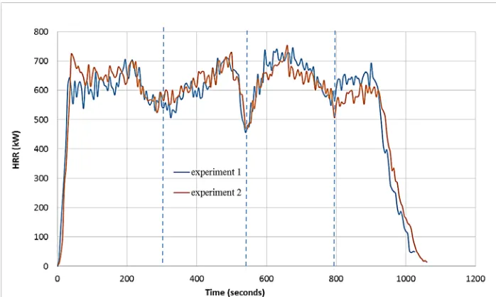
Figure 8. HRR repeatability during experiments. Dashed line represents jumping of flame (ignition) to the next row of trays.

4 EXPERIMENTAL AND NUMERICAL RESULTS

4.1 Experimental results.

tests are presented in Figure 8. Excellent repeatability of the test result is observed in this figure. Four stages of burning process correspond to the burning of fuel in each row of the trays can be identified in the figure and this was also observed during the experiments. The ignition and burning of the fuel, and location of the flame in different trays were observed in the experiments and are presented in Table 3. The values of Table 3 were also verified from video observation and HRR curves presented in Figure 8 (indicated by dashed lines). Some related photos, captured during the tests, are also presented in Figure 9.

(a) Combustion at tray 7-8. (b) Combustion at tray 5-6 (c) Combustion at tray 1-2 Figure 9. Burning behaviour during tests.

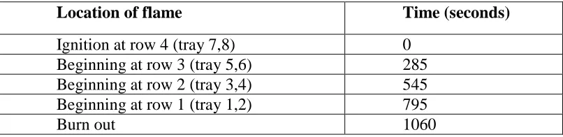
Table 3. Visual observation of flame movement

Location of flame Time (seconds)

Ignition at row 4 (tray 7,8) 0

Beginning at row 3 (tray 5,6) 285

Beginning at row 2 (tray 3,4) 545

Beginning at row 1 (tray 1,2) 795

Burn out 1060

4.2 Numerical results.

The HRRs of fires obtained from the experiments were prescribed into FDS 6 to see how well FDS reproduces prescribed input HRRs. In the input file, the description of fire was created to be similar to the experiment.

Selection of Computational Grid

To make quantitative comparison between experimental and numerical result, it is essential to select the simulation which is grid converged. In this study, simulations were conducted using 50 mm as well as 25mm and 12.5mm grid sizes. The use of 25 and 12.5 mm grids for a domain of 4 m × 2 m × 0.6 m in size demand a huge computational resource for simulation. Therefore, a supercomputer was used to meet the computational requirements. For the same reason simulation with 12.5mm grid was conducted for up to 300 secs.

the simulation. In this case, the gas temperature of the front row tray is compared and presented in Figure 10(b). It is observed that the grid convergence is obtained with 25 mm size of grid as the results of 25 and 12.5 mm nominally converged.

(a) HRR (b) Gas Temperature at ‘Under location’ of tray 7-8 Figure 10. HRR and temperature from the experiment and simulation.

A statistical analysis is conducted to assess the quantitative difference of the data compared to a reference value. Here, we have calculated quantitative difference of the data produced with 25 mm and 50 mm grid and then quantitative difference of the data produced with 12.5 mm and 25 mm grid. The method by Ierardi et al. [19] is adopted to calculate the error analysis. According to the approach, quantitative difference for an individual varaible can be measured by,

𝜉𝜉 =(ℛ − 𝜓𝜓)_𝜓𝜓 (6)

Where, ℛ and 𝜓𝜓 are predicted and the reference values, respectively. The mean quantitative difference can be calculated by the absolute values of error in the individual points 𝑛𝑛.

𝜉𝜉𝑚𝑚=

∑𝑛𝑛𝑖𝑖=1��ℛ − 𝜓𝜓_{𝜓𝜓 ��}

𝑛𝑛 (7)

The mean quantitative difference of among FDS predictions has been calculated and presented in Table 4. From this quantitative difference analysis, it has been decided that in this study, 25mm grid size simulation results would be used.

Table 4: Analysis of mean relative error of the FDS prediction.

Variables

Mean quanative difference (%) between data

Refered figure number 25mm grid vs 50mm grid 12.5mm grid vs 25mm grid

HRR 4.9 1.7 Figure 10(a)

Gas temperature_under_ tray 7-8 14.2 8.6 Figure 10(b)

Reproducing Experimental HRR

to the experimental data for the whole combustion process. There is a short period at the beginning where the FDS results were less than those in the experiment. During this period, the HRR from the FDS could not reach the peak of HRR.

Figure 11. Comparison of HRR obtained from the experiment and simulation.

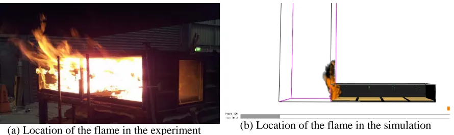
It is likely that this difference was due to the flame location during the first stage of burning of the fuel, which is also shown in Figure 12. As seen in Figure 12(b), at 200 seconds the burning process took place at the lips of trays 7 and 8. However, in the experiment, the flame was above the trays, largely inside the enclosure. The flame front in the simulation deprives some part of the ejected fuel from the trays 7 and 8 of oxygen.

(a) Location of the flame in the experiment (b) Location of the flame in the simulation

Figure 12. Location of the flame at 200 seconds in the experiment and simulation.

(a) 294 sec (b) 551 sec (c) 799 sec Figure 13. The flame location during simulation.

4.3 Comparison of Experimental and Numerical results- other parameters

The gas temperatures were measured above each row of the trays in the experiment and predicted in the simulation. The comparison of temperature between them is presented in Figure 14. It is to be noted that flames over trays in the same row is not always symmetric due to its turbulent nature. Therefore, temperatures at the corresponding locations for trays 7 & 8, 5 & 6, 3 & 4 and 1 & 2 are averaged. There were four thermocouples above each tray and their locations are shown in Figure 7. Similarly, the radiation fluxes emitted from the fire were measured in the experiment and compared with the prediction of that of the simulation. The results are shown in Figure 16. The details of the comparison are described below.

Comparison of gas temperatures

Generally, the simulation results deviated from the experimental results while the fire was located above trays 7 and 8 except first 45 sec. During this stage the temperature from simulation was much lower than that of the experiment for all of the locations of the thermocouple. It is likely that this difference was the result of (1) the difference in HRR explained in previous section and (2) the flame location during the first stage, which is shown in Figure 12. As seen in Figure 12(b), at 200 seconds the burning process happened above row 4 (tray 7 and 8). However, in the experiment, the flame made direct contact with the thermocouples above tray 7 and 8 while in the simulation, at the same timeline moment, the flame stayed at the lips of the trays and did not make contact with the thermocouples. Interestingly, after 325 seconds, the moment the flame in the simulation moved back to the next row (row 3 with trays 5 and 6, as seen in Figure 6), the simulation results for all thermocouple locations (especially under and middle locations) showed a much lower deviation from the experimental data.

For under and middle locations above trays 5 and 6, FDS provided more close results with the experimental measurements after about 575 seconds as shown in Figure 14 (d) and (e). This was the moment the flame passed tray 5 and 6 and the flame front moved back to trays 3 and 4. During the period from 0 to 575 seconds, the difference between the simulation and experimental results was significant, especially the gas temperature. This was ~250oC up to 325 sec and ~100oC between 325 and 575 sec. This might be the result of the flame location and the lack of contact between the flame and the thermocouples in the simulation, as was apparent for the comparison of temperatures in row 4 (tray 7 and 8).

After the flame front moved back beyond row 2, results for thermocouple locations above this row were well predicted by FDS. However, prior to flame reaching row 2 the prediction was also good. Interestingly, the temperature above row 1 (tray 1 and tray 2) did not follow the same pattern as the previous row of trays. The temperature above row 1 (tray 1 and 2) was quite close to that in the experiment, even during the period in which combustion took place above this row. As illustrated in Figure 13(c), the flame at 799 seconds in the simulation tended to be in direct contact with the thermocouples above the row 1 fuel tray. This behaviour explains why the simulation result of temperature data matched well with the experimental measurement, as shown in Figure 14 (d).

(a) Tray 7-8 under (b) Tray 7-8 middle (c) Tray 7-8 low

(d) Tray 5-6 under (e) Tray 5-6 middle (f) Tray 5-6 low

(g) Tray 3-4 under (h) Tray 3-4 middle (i) Tray 3-4 low

(j) Tray 1-2 under (k) Tray 1-2 middle (l) Tray 1-2 low

Figure 14. Comparison of gas temperatures.

Exceptionally temperatures above trays 1 and 2 are well matched throughout the simulation. Comparison of surface temperatures

Figure 15 presents comparison of surface temperatures over four trays. It is to be noted that to predict the surface temperature, very fine computational grid is required to resolve thermal boundary layer. This is out of the scope of this study. Despite using relatively coarse grid near the solid surface Figure 15 shows that peak temperatures obtained in both experimental and numerical study are quite close.

(a) Comparison for tray 7 and 8 (b) Comparison for tray 5 and 6

(c) Comparison for tray 3 and 4 (d) Comparison for tray 1 and 2

Figure 15. Comparison of surface temperatures.

Comparison of radiation flux

Figure 6 shows the locations of radiometers for collecting data of heat flux rate from the flame in both experiment and simulation. However, the data from radiometer 1 might be unreasonable due to soot covering the surface of this radiometer. Therefore, only data from radiometer 2, which was located at the opening side of the compartment, is presented in Figure 16.

It can be seen from Figure 16 that the heat flux from the simulation were quite closed to experimental data except the first period of combustion process up to about 285 seconds when the flame was protruding out as observed in Figure 12(b).

7 CONCLUSION

In this study, both scaled tests and numerical simulation were carried out to find out the deep rig dimension that could be used to simulate fire behavior using CFD based fire model such as FDS 6. The main conclusions and findings of this study can be summarized as below:

Redesigning of an experimental rig based on empirical models (VU model and Kawagoe equation) as well as FDS was carried out, so that tests with the designed rig can be realistically simulated by FDS. However, the HRR determined by the Kawagoe model could not be reproduced using the FDS model when that HRR was prescribed as input, while the HRR determined by the VU model was well reproduced by the simulation with FDS for a deep enclosure.

The HRR obtained through the experiments was prescribed into FDS and observed that it could reasonably reproduce the HRR. FDS’ combustion model (reaction between gaseous fuel and oxygen) works well in this configuration when evaporation process is not modelled, rather prescribed via HRR.

Temperature (surface and air) is an outcome of HRR. When the HRR from the experiments was prescribed into the FDS, the temperature prediction by the FDS at a specific thermocouple could be reasonably predicted after the flame front had crossed or prior to reaching that thermocouple, depending on the thermocouple location. Otherwise, FDS was unable to predict the temperature well at a specific thermocouple location when the flame front stayed at the lips of the corresponding fuel trays. Radiation flux was also well predicted by FDS except for the first period of combustion up to 285 seconds when a major part of the heat released outside the enclosure. In this study, a liquid evaporation model was not tested. Experimental results could be used for validation of the evaporation model without prescribed HRR. If the evaporation model is well validated, FDS could be used for developing improvements in fire severity models, such as the VU model.

REFERENCES

1 Moinuddin, K, and Thomas, I.R. An experimental study of fire development in deep enclosures and a new HRR–time–position model for a deep enclosure based on ventilation factor. Fire and Materials, 2009; 33:157–185. DOI: 10.1002/fam.986.

2 Kawagoe K. Fire behaviour in rooms. Report No. 27, Building Research Institute, Tokyo, 1958.

3 Jolly, S, Saito, K, Scale Modeling of Fires with Emphasis on Room Flashover Phenomenon. Fire Safety Journal, 18, 1992, pp. 139 - 182.

4 Venkatasubbaiah, K. and Jaluria, Y. Numerical simulation of enclosure fires with horizontal vents. Numerical Heat Transfer, Part A, 62: 179–196, 2012. DOI: 10.1080/10407782.2012.677361.

and Wide Enclosures. Fire Safety Science-Proceedings of the Sixth International Symposium, 1999, pp 941-952.

6 Beji, T., Ukleja, S., Zhang, J., and Delichatsios, M. A. Fire behaviour and external flames in corridor and tunnel-like enclosures. Fire and Materials, 2012; 36:636–647. DOI: 10.1002/fam.1124.

7 Thomas, IR et al, Fire Resistance and Non-combustibility; Evaluation of Fire Resistance Levels: Techniques, Data and Results. Project Report FCRC-PR 01-02, FCRC Project 3 Part 2, Australia, 1999. 8 SFPE Task Group, Engineering Guide- Fire Exposures to Structural Elements, SFPE, Bathesda, MD, May 2004.

9 Magnussion, SE, Thelandersson, S, Temperature-Time Curves of Complete Process of Fire Development, Civil Engineering and Building Construction Series, ACTA Polytechnica Scandinavica, 1970. 10 Thomas, I.R, Moinuddin, K., Bennetts, I.D. Fire Development in a Deep Enclosure. Fire safety science– proceedings of the eighth international symposium, 2005, pp. 1277-1288.

11 McGrattan, K., Hostikka, S., McDermott, R., Floyd, S., Weinschenk, C and Overholt, K., Fire Dynamics Simulator (Version 6), Technical Reference Guide-Volume 1: Mathematical Model, NIST Special Publication 1018-6, National Institute of Standards and Technology, Gaithersburg, MD, USA, 2014.

12 McGrattan, K., Hostikka, S., McDermott, R., Floyd, S., Weinschenk, C and Overholt, K., Fire Dynamics Simulator (Version 6), User's Guide, NIST Special Publication 1019-6, National Institute of Standards and Technology, Gaithersburg, MD, USA, 2014.

13 Feasey, R 1999, Post-flashover Design Fires, Master thesis, Department of Civil Engineering University of Canterbury Christchurch, New Zealand.

14 Drysdale, D 2011, An Introduction to Fire Dynamics, 3rd edition, John Wiley & Sons, UK.

15 Thomas PH, Heselden AJM. Fully developed fires in single compartments. A cooperative research programme of the conseil internationale du batiment. CIB Report No. 20, Fire Research Note 923, U.K., 1972.

16 Incropera, F.P., Dewitt, D.P., Bergman T.L., 2006. Fundamental of Heat and Mass Transfer. 6th edn. Wiley. 2006.

17 Zou GW, Chow WK, Evaluation of the Field Model, Fire Dynamics Simulator, for a Specific Experimental Scenario, Journal of Fire Protection Engineering, 15 (2005) 77- 92.

18 Moinuddin, K., Al-Menhali, J. S., Prasannan, K., Thomas. I. R, Rise in structural steel temperatures during ISO9705 room fires. Fire Safety Journal 46, 2011, pp. 480–496.