Comparison of stochastic and machine learning methods for multi-step
ahead forecasting of hydrological processes
Georgia Papacharalampous1,*, Hristos Tyralis2, and Demetris Koutsoyiannis3
1 Department of Water Resources and Environmental Engineering, School of Civil
Engineering, National Technical University of Athens, Iroon Polytechniou 5, 157 80 Zografou, Greece; [email protected]; ORCID:
0000-0001-5446-954X
2 Air Force Support Command, Hellenic Air Force, Elefsina Air Base, 192 00 Elefsina,
Greece; [email protected]; ORCID: 0000-0002-8932-4997
3 Department of Water Resources and Environmental Engineering, School of Civil
Engineering, National Technical University of Athens, Iroon Polytechniou 5, 157 80 Zografou, Greece; [email protected]; ORCID: 0000-0002-6226-0241
* Correspondence: [email protected], tel: +30 69474 98589
This is a pre-print of an article published in Stochastic Environmental Research and
Risk Assessment (2019). The final authenticated version is available online at:
https://doi.org/10.1007/s00477-018-1638-6
Abstract: Research within the field of hydrology often focuses on the statistical problem of comparing stochastic to machine learning (ML) forecasting methods. The comparisons performed are based on case studies, while a study providing large-scale results on the
subject is missing. Herein, we compare 11 stochastic and 9 ML methods regarding their
multi-step ahead forecasting properties by conducting 12 extensive computational experiments based on simulations. Each of these experiments uses 2 000 time series
generated by linear stationary stochastic processes. We conduct each simulation
experiment twice; the first time using time series of 100 values and the second time using time series of 300 values. Additionally, we conduct a real-world experiment using 405
mean annual river discharge time series of 100 values. We quantify the performance of
the methods using 18 metrics. The results indicate that stochastic and ML methods perform equally well.
Key Words: no free lunch theorem; random forests; river discharge; stochastic hydrology; support vector machines; time series
2
1.
Introduction
1.1
Background information
The fundamental problem of statistically producing point forecasts of univariate time
series by exploiting information from their past values only (hereafter, “forecasting”,
unless specified differently) is of traditional interest to hydrological scientists (Yevyevich 1987). Right after the introduction of the currently classical Autoregressive Integrated
Moving Average (ARIMA) models by Box and Jenkins (1968), Carlson et al. (1970) used several stationary models of this specific family, i.e. Autoregressive Moving Average
(ARMA) models, to forecast the evolution of four annual time series of streamflow
processes. Today the available models for time series forecasting are numerous and can be classified according to De Gooijer and Hyndman (2006) into eight categories, i.e. (a)
exponential smoothing, (b) ARIMA, (c) seasonal models, (d) state space and structural
models and the Kalman filter, (e) nonlinear models, (f) long-range dependence models, e.g. the family of Autoregressive Fractionally Integrated Moving Average (ARFIMA)
models, (g) Autoregressive Conditional Heteroscedastic/Generalized Autoregressive
Conditional Heteroscedastic (ARCH/GARCH) models and (h) count data forecasting. The models from the categories (a)-(g) are of potential interest in hydrology, while they can
be implemented for both one- and multi-step ahead forecasting.
The theoretical properties of the models of categories (a)-(d), (f), (g) (hereafter,
referred to as “stochastic”) have been more or less investigated, in contrast to those of the nonlinear models and in particular the Machine Learning (ML) algorithms, also referred
to in the literature as black-box models. These two main categories of models are known
to represent two different cultures in statistical modelling, the data modelling culture and the algorithmic modelling culture (Breiman 2001b). The former assumes that an
analytically formulated stochastic model is behind the generation of the data, while the
latter that behind this process is something complex and unknown, which does not have to be analytically formulated, as long as a purely algorithmic model can offer high forecast
accuracy. In other words, profoundly understanding and properly modelling the (future)
behaviour of a process are strongly connected within the data modelling culture, but completely irrelevant within the algorithmic modelling culture. The distinction between
causal explanation, prediction and description is acknowledged and clarified in terms of
3
separation of models with respect to the “stochastic-ML dipole” actually corresponds to a striking difference in their forecasting performance.
What cannot be questioned, on the other hand, is the popularity that the various ML
forecasting methods have gained in many scientific fields, including hydrology. Amongst
the most popular ML algorithms are the Neural Networks (NN), Random Forests (RF) and Support Vector Machines (SVM). The SVM are presented in their current form by Cortes
and Vapnik (1995) (see also Vapnik 1995, 1999), while RF by Breiman (2001a). For the
implementation of the NN for time series forecasting the reader is referred to Zhang et al. (1998) and Zhang (2001). Regarding the use of SVM for this specific purpose, a review can
be found in Sapankevych and Sankar (2009). The large number of the relevant
applications of the NN and SVM algorithms in the field of hydrology is imprinted in Maier and Dandy (2000) and Raghavendra and Deka (2014) respectively, while Abrahart et al.
(2012) collectively review the NN streamflow forecasting and rainfall-runoff applications
(examples of the latter can be found, for instance, in De Vos (2013), although rainfall-runoff applications are a completely different problem since it is based on the use of
exogenous variables, see also the discussion in Section 4). The RF algorithms, on the other
hand, are barely used for the forecasting of hydrological processes.
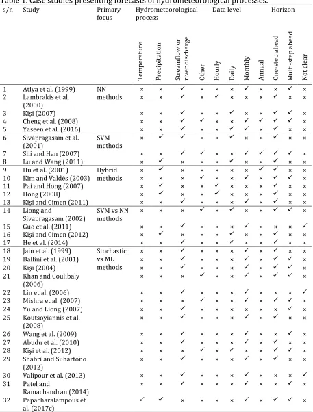
In Table 1 we present some literature information on hydrometeorological time series forecasting to explore the related background and facilitate the following discussion. As it
is apparent, hydrological research often focuses on ML or hybrid (e.g. a combination of
ARMA and ML) forecasting methods and, in particular, on the comparison between stochastic (mainly ARMA and ARFIMA) and ML methods. However, the culture of
assessing the performance of forecasting methods on large datasets is not customary in
hydrology. Therefore, the assessment is performed within case studies. Concerning the testing procedure, while the available metrics for the assessment of the forecast quality
are a lot, most of the studies use only a few (Krause et al. 2005), understating the
4
Table 1. Case studies presenting forecasts of hydrometeorological processes.
s/n Study Primary
focus
Hydrometeorological process
Data level Horizon
T em p er at u re P re ci p it at io n St re am fl o w o r ri ve r d is ch ar ge O th er H o u rl y D ai ly M o n th ly A n n u al O n e-st ep a h ea d M u lt i-st ep a h ea d N o t cl ea r
1 Atiya et al. (1999) NN methods
× × × × × × × ×
2 Lambrakis et al. (2000)
× × × × × × × ×
3 Kişi (2007) × × × × × × ×
4 Cheng et al. (2008) × × × × ×
5 Yaseen et al. (2016) × × × × × × ×
6 Sivapragasam et al. (2001)
SVM methods
× × × × × × ×
7 Shi and Han (2007) × × × × ×
8 Lu and Wang (2011) × × × × × × × ×
9 Hu et al. (2001) Hybrid methods
× × × × × × × ×
10 Kim and Valdés (2003) × × × × × × ×
11 Pai and Hong (2007) × × × × × × × ×
12 Hong (2008) × × × × × × × ×
13 Kişi and Cimen (2011) × × × × × × × × 14 Liong and
Sivapragasam (2002)
SVM vs NN methods
× × × × × × ×
15 Guo et al. (2011) × × × × × × × ×
16 Kişi and Cimen (2012) × × × × × × × ×
17 He et al. (2014) × × × × × × × ×
18 Jain et al. (1999) Stochastic vs ML methods
× × × × × × × ×
19 Ballini et al. (2001) × × × × × × ×
20 Kişi (2004) × × × × × × ×
21 Khan and Coulibaly (2006)
× × × × × × ×
22 Lin et al. (2006) × × × × × × × ×
23 Mishra et al. (2007) × × × × × × ×
24 Yu and Liong (2007) × × × × × × × × ×
25 Koutsoyiannis et al. (2008)
× × × × × × × ×
26 Wang et al. (2009) × × × × × × × ×
27 Abudu et al. (2010) × × × × × × × ×
28 Kişi et al. (2012) × × × × × × ×
29 Shabri and Suhartono (2012)
× × × × × × × ×
30 Valipour et al. (2013) × × × × × × × × 31 Patel and
Ramachandran (2014)
× × × × × × × ×
32 Papacharalampous et
al. (2017c)
× × × × × ×
Researchers have long been chasing the most accurate forecast for their data, a
“universally best technique”. On the other hand, there is an argument that it is the data and
5
invest more on probabilistic forecasting (e.g. using Bayesian statistics as in Tyralis and Koutsoyiannis 2014) and less on point forecasting (Krzysztofowicz 2001). In fact, the
opinions on forecast evaluation are often diverging, as they tend to depend on the perspective from which the forecasts are examined. An interesting study on this subject
can be found in Murphy (1993). The latter identifies three criteria for this specific
evaluation, which are adopted as a foundation for further discussion in later studies, e.g.
Ramos et al. (2010) and Weijs et al. (2010). These criteria are (1) the consistency during the forecasting process, (2) the quality or the correspondence between the forecasts and
the target values and (3) the value or the profit that the forecast provide to the decision
makers. Weijs et al. (2010) note that criterion (2) concerns more the pure science, while criterion (3) is closer related to the decisions made within the engineering applications
(of science), rather than science itself. Thus, only a few studies are dedicated to criterion (3), such as Ramos et al. (2010) and Ramos et al. (2013), while the greatest part of the
literature focuses on criterion (2). The latter likewise applies to the present study and to
all of its references aiming to deal with the modelling issue (which model should I use?) within specific hydrological concepts.
Regarding the so far conducted comparisons between forecasting methods, their majority in all scientific fields is based on case studies. Nevertheless, in some few cases
beyond the field of hydrology the number of the examined real-world time series is quite
large. These time series are realizations of several phenomena, which however are fundamentally different from being hydrological, and their examination includes concepts
that are rather inappropriate in hydrological terms (e.g. paying attention to small
quantitative differences in the forecasting performance of the methods). Examples of such studies can be found in Makridakis et al. (1987), Makridakis and Hibon (2000) and Ahmed
et al. (2010), which examine 1 001, 3 003 and 1 045 time series respectively. Within these studies a statistical analysis is performed and the results are presented correspondingly.
Furthermore, the literature includes two studies (Zhang 2001; Thissen et al. 2003) in
which the performance of the methods is assessed on simulated time series from linear stochastic processes. The scale of the simulation experiment is small in both cases.
Thissen et al. (2003) examine one long time series from the ARMA family, while Zhang
(2001) examine 8 stochastic processes from the ARMA family and 30 simulated time series for each stochastic process. The forecasting methods are ARMA models, NN and
6
and Hibon (1987), Makridakis and Hibon (2000) and Ahmed et al. (2010) do not focus their comparisons on the stochastic-ML dipole.
Admittedly, the studies mentioned in the previous paragraph pursue generalized
results to greater extent than most of the available studies. However, the gap still remains.
What specifically needs to be addressed is whether the stochastic-ML dipole actually corresponds to a clear difference in the forecasting performance of the methods,
especially in the light of published studies, which claim that they found a technique better
than others. Given the fact that each forecasting case is indisputably unique, this task would necessarily require the examination of a sufficiently large and representative
sample of forecasting cases within the same (properly designed) methodological
framework. Some suggestions for the design of large-scale studies are available in Alpaydin (2010). Extensive simulations combined with statistical analysis and
benchmarking can constitute, nevertheless, a highly effective approach to solving the
problem under discussion. In more detail, for the generalized comparison of stochastic and ML forecasting methods, a sufficient number of different and representative of the
underlying phenomena time series could be used for the estimation of the expected
performance of several forecasting methods regarding several criteria of interest. The need of using simulated time series to assess the performance of forecasting methods is
emphasized by forecasting experts (Bontempi 2013). The analytical approach in
assessing the performance of ML algorithms is usually not possible; therefore, the only alternative approach is using simulations. Apparently, the larger the scale of the
simulation experiments, the more general would be the results. Real-world experiments
of large-scale could be used to complement the results of the simulation experiments in alignment with specific applications.
1.2
The present study
In the context described in the above section, we perform an extensive comparison
between several stochastic and ML methods for the forecasting of hydrological processes by conducting large-scale computational experiments based on simulations. The
comparison refers to the multi-step ahead forecasting properties of the methods,
although one-step ahead forecasting is also of practical and scientific interest. The simulated time series are 48 000 in total, while they are generated by linear stationary
7
In fact, stationary models, in contrast to the non-stationary, are established as the appropriate modelling choice when dealing with natural processes, unless tangible and
quantitative information that can fully support a deterministic description (not based on data but on physical laws) of change in time are available (Koutsoyiannis 2011;
Koutsoyiannis and Montanari 2015). Additionally to the simulation experiments, we
examine 405 real-world time series. Our aim is to fill the gap detected in the literature by
providing large-scale results and useful insights on the comparison of stochastic and ML forecasting methods for the case of hydrological time series forecasting, with an emphasis
on river discharge processes. A strength (and limitation) of the present study (implied by
its aim) is the adopted approach to the problem, i.e. the algorithmic one.
The present study was first presented by Papacharalampous et al. (2017a), while a preliminary research on the subject was conducted for the Postgraduate Thesis of the first
author (Papacharalampous 2016). Subsequently, we provide some basic information
about the large-scale companion studies of this paper. Papacharalampous et al. (2017b) examine the problem of error evolution in hydrological multi-step ahead forecasting,
while Tyralis and Papacharalampous (2017) improve the performance of RF in one-step
ahead forecasting of geophysical processes. Papacharalampous et al. (2018b) also focuses on the problem of one-step ahead forecasting with the aim to provide large-scale results
on the latter in geoscience. These three studies examine simulated, as well as real-world
datasets. In detail, they examine 12 000 simulated and 92 monthly streamflow time series, 16 000 simulated and 135 annual temperature time series, and 24 000 simulated, 185
annual temperature and 112 annual precipitation time series respectively. Finally,
Papacharalampous et al. (2018c) produce multi-step ahead forecasts for 985 monthly temperature and 1 552 monthly precipitation time series aiming at the investigation of
the predictability of these processes. All the time series examined by the present study and its companions are short, as it is expected for the hydrometeorological time series.
A subsequent to Papacharalampous (2016) and Papacharalampous et al. (2017a) study by Makridakis et al. (2018) focuses on a similar investigation to the present paper,
although in a different field and under a different experimental setting. In particular
Makridakis et al. (2018) conclude that at the moment the statistical methods are better compared to the machine learning methods, while as shown here the performance of all
8
2.
Methodology
In Section 2 we present the basic methodological elements of this study, while the reader
is referred to the supplementary material for a brief theoretical background, as also to the scientific literature for a more complete coverage of the relevant theory.
2.1
Simulated processes
We simulate time series according to several stochastic models from the frequently used
families of ARMA and ARFIMA. This modelling approach is considered appropriate for the achievement of our aim and has been widely applied in hydrology (e.g. Montanari et al.
(1997, 2000), Ballini et al. (2001), Wang et al. (2009), Valipour et al. (2013)). The
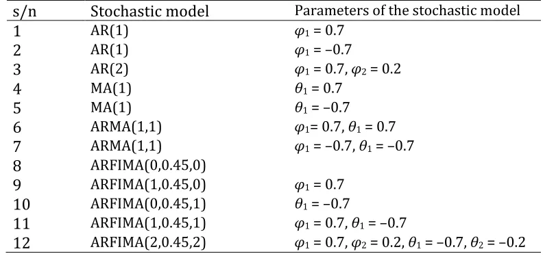
simulated stochastic processes are presented in Table 2, while for the related definitions the reader is referred to the report entitled “Definition of the stochastic processes’’ of the
supplementary material. These 12 stochastic models correspond to different types of
autocorrelation. We use the arima.sim built in R algorithm (R Core Team 2017) to simulate the ARMA(p, q) processes and the fracdiff.sim algorithm of the fracdiff R package
(Fraley et al. 2012) to simulate the ARFIMA(p, d, q) processes.
Table 2. Simulated stochastic processes of the present study. Their definitions are given in the supplementary material.
s/n Stochastic model Parameters of the stochastic model
1 AR(1) φ1 = 0.7
2 AR(1) φ1 = –0.7
3 AR(2) φ1 = 0.7, φ2 = 0.2
4 MA(1) θ1 = 0.7
5 MA(1) θ1 = –0.7
6 ARMA(1,1) φ1= 0.7, θ1 = 0.7
7 ARMA(1,1) φ1 = –0.7, θ1 = –0.7
8 ARFIMA(0,0.45,0)
9 ARFIMA(1,0.45,0) φ1 = 0.7
10 ARFIMA(0,0.45,1) θ1 = –0.7
11 ARFIMA(1,0.45,1) φ1 = 0.7, θ1 = –0.7
9
2.2
Real-world time series
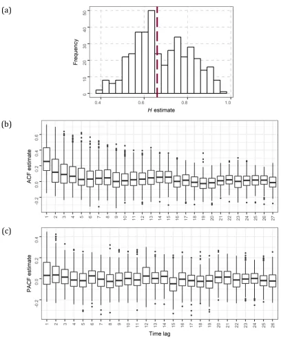
We examine 405 mean annual discharge time series of 100 values, sourced from GRDC
(2017). For the exploration of these time series we calculate the sample Autocorrelation Function (ACF) and the sample Partial Autocorrelation Function (PACF). The side-by-side
boxplots of the ACF and PACF estimates are presented in Figure 1. The Hurst-Kolmogorov
behaviour (HK behaviour) is a common property of geophysical properties (e.g. Tyralis and Koutsoyiannis 2011). To describe the HK behaviour of discharge we estimate the
Hurst parameter H of all time series using the mleHK algorithm of the HKprocess R package (Tyralis 2016), which implements the maximum likelihood method (Tyralis and
Koutsoyiannis 2011). The parameter H takes values in the interval (0, 1). The larger it is
the larger the magnitude of the HK behaviour, which can be modelled by an ARFIMA(0, d, 0) model. A histogram of the H estimates is presented in Figure 1. By the
examination of the latter we observe that the magnitude of the long-range dependence in
10 (a)
(b)
(c)
Figure 1. (a) H, (b) ACF, (c) PACF estimates of the real-world time series. Data source: GRDC (2017). The red dashed line in the upper graph denotes the median of the H
estimates.
2.3
Forecasting methods
We compare 11 stochastic to 9 ML forecasting methods. The stochastic methods are classified into five main categories as presented in Table 3. Similarly, the ML methods are
classified into three main categories as presented in a compact form in Table 4 and Table
11
Table 3. Stochastic forecasting methods. The forecasting methods are available in code form in the supplementary material.
s/n Abbreviated name Category
1 Naïve Simple
2 RW
3 ARIMA_f ARIMA
4 ARIMA_s 5 auto_ARIMA_f 6 auto_ARIMA_s
7 auto_ARFIMA ARFIMA
8 BATS State Space
9 ETS_s
10 SES Exponential Smoothing 11 Theta
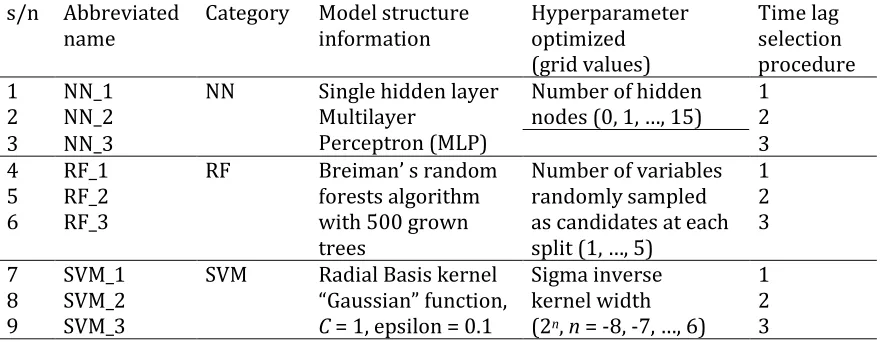
Table 4. ML forecasting methods. The time lag selection procedures adopted are defined in Table 5. The forecasting methods are available in code form in the supplementary material.
s/n Abbreviated name
Category Model structure information Hyperparameter optimized (grid values) Time lag selection procedure 1 NN_1 NN Single hidden layer
Multilayer
Perceptron (MLP)
Number of hidden nodes (0, 1, …, 15)
1
2 NN_2 2
3 NN_3 3
4 RF_1 RF Breiman’ s random forests algorithm with 500 grown trees
Number of variables randomly sampled as candidates at each split (1, …, 5)
1
5 RF_2 2
6 RF_3 3
7 SVM_1 SVM Radial Basis kernel “Gaussian” function, C = 1, epsilon = 0.1
Sigma inverse kernel width (2n, n = -8, -7, …, 6)
1
8 SVM_2 2
9 SVM_3 3
Table 5. Time lag selection procedures adopted for the ML methods. The forecasting methods are available in code form in the supplementary material.
s/n Time lags
1 The corresponding to an estimated value for the ACF using the acf R algorithm (built in R algorithm), i.e. the time lags 1, …, 19 for a time series of 90 values and the time lags 1, …, 24 for a time series of 290 values
2 The corresponding to a statistical important estimated value for the ACF using the acf R algorithm (built in R algorithm). If there is no statistical important estimated value for the ACF, the corresponding to the largest estimated value
3 According to the nnetar R function (package forecast), i.e. the time lags 1, …, n, where n is the number of AR parameters that are fitted to the time series data using the ar R algorithm (built in R algorithm)
We use two simple forecasting methods in the comparisons. The Naïve forecasting
method, one of the most commonly used benchmarks (Hyndman and Athanasopoulos
2013; Pappenberger et al. 2015), simply sets all forecasts equal to the last value. The RW forecasting method, a variation of the Naïve forecasting method, is equivalent to drawing
12
and Athanasopoulos 2013). The stochastic methods also include the ARIMA and ARFIMA methods. These five methods apply the maximum likelihood method to estimate the
values of the parameters of the AR and MA parts of the models. For the ARIMA_f and ARIMA_s forecasting methods the numbers of the AR (p) and MA (q) parameters are set
to be the same to those used in the simulated processes, while the number of differencing
(d) is set to be zero. The auto_ARIMA_f and auto_ARIMA_s methods estimate the values of
p, d, q of the ARIMA model using the Akaike Information Criterion with a correction for
finite sample sizes (AICc), as described in Hyndman and Athanasopoulos (2013). The
same applies to the auto_ARFIMA method for the estimation of the values of p, d, q of the
ARFIMA models. We note that ARIMA_s and auto_ARIMA_s are simulation models.
The BATS and ETS_s forecasting methods use the point forecasts from an exponential smoothing state space model with several key features, i.e. capability of performing
Box-Cox transformation and/or including ARMA errors correction, Trend and Seasonal
components (BATS), also allowing an optimal model selection using the Akaike Information Criterion (AIC), and an exponential smoothing state space simulation model
with automatic selection of the Error, Trend and Seasonal components (ETS) respectively.
We additionally include the SES (Simple Exponential Smoothing) and Theta forecasting methods in the comparisons. The latter method was presented by Assimakopoulos and
Nikolopoulos (2000) and performed well in the M3-Competition (Makridakis and Hibon
2000). The reader is referred to Hyndman et al. (2008) and Hyndman and Athanasopoulos (2013) for the theoretical background of the exponential smoothing and space state
models.
Regarding the NN, the RF and the SVM forecasting methods, there are some additional
concerns to the selection of the algorithms, originating from the nature of the ML methods. The choices to be considered for the selection of the time lags used to build the regression
matrix (input data matrix), as well as the choices for the values of the hyperparameters of
the models (e.g. the hidden nodes in a NN model), are many. Usually, hyperparameters are not automatically decided by the ML algorithm during the fitting process. A fact is that
the ML models are by design rather more flexible than needed in most cases and, thus,
hyperparameter optimization is often used to detect and prevent overfitting as much as possible. In Tables 4 and 5 we summarize the basic information about the model
13
We apply the stochastic methods using mainly the R package forecast (Hyndman and Khandakar 2008, Hyndman et al. 2017) and the ML methods using the R package rminer
(Cortez 2010, 2016) and the nnetar algorithm from the R package forecast (the latter is the NN_3 forecasting method), as also several built in R algorithms. The R package rminer
uses the nnet algorithm of the nnet R package (Venables and Ripley 2002), the
randomForest algorithm of the randomForest R package (Liaw and Wiener 2002) and the
ksvm algorithm of the kernlab R package (Karatzoglou et al. 2004) for the application of the NN, the RF and the SVM methods respectively.
2.4
Metrics
The metrics used for the comparative assessment of the forecasting methods are
classified into five main categories according to the criteria of Table 6. They provide assessment regarding two types of accuracy, the capture of the variance and the
correlation. By Type 1 accuracy we mean the closeness of the forecasted time series to the
actual, while by Type 2 accuracy we mean the closeness of the mean of the forecasted values of each time series to the mean of the actual ones. The definitions of the metrics
are listed in the report entitled “Definition of the metrics’’ of the supplementary material,
while the reader is also referred to Nash and Sutcliffe (1970), Kitanidis and Bras (1980), Yapo et al. (1996), Krause et al. (2005), Criss and Winston (2008), Gupta et al. (2009),
Zambrano-Bigiarini (2014) for further information.
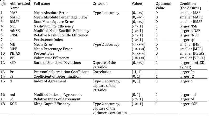
Table 6. Metrics used in the present study. Their definitions are given in the supplementary material.
s/n Abbreviated Name
Full name Criterion Values Optimum
Value
Condition (the desired) 1 MAE Mean Absolute Error Type 1 accuracy [0, +∞) 0 smaller MAE
2 MAPE Mean Absolute Percentage Error [0, +∞) 0 smaller MAPE
3 RMSE Root Mean Square Error [0, +∞) 0 smaller RMSE
4 NSE Nash-Sutcliffe Efficiency (-∞, 1] 1 larger NSE
5 mNSE Modified Nash-Sutcliffe Efficiency (-∞, 1] 1 larger mNSE 6 rNSE Relative Nash-Sutcliffe Efficiency (-∞, 1] 1 larger rNSE
7 cp Persistence Index (-∞, 1] 1 larger cp
8 ME Mean Error Type 2 accuracy (-∞,+∞) 0 smaller |ME|
9 MPE Mean Percentage Error (-∞,+∞) 0 smaller |MPE|
10 PBIAS Percent Bias (-∞,+∞) 0 smaller |PBIAS|
11 VE Volumetric Efficiency (-∞,+∞) 1 smaller |VE - 1|
12 rSD Ratio of Standard Deviations Capture of the variance
[0, +∞) 1 larger min{rSD, 1/rSD} 13 Pr Pearson’ s Correlation Coefficient Correlation [-1, 1] 1 larger Pr
14 r2 Coefficient of Determination [0, 1] 1 larger r2
15 d Index of Agreement Type 1 accuracy, capture of the variance
[0, 1] 1 larger d
16 md Modified Index of Agreement [0, 1] 1 larger md
17 rd Relative Index of Agreement (-∞, 1] 1 larger rd
18 KGE Kling-Gupta Efficiency Type 2 accuracy, capture of the variance, correlation
14
2.5
Methodology outline
For the comparison of the forecasting methods (see Section 2.3) we conduct 12 large-scale
computational experiments based on simulations. Within each of the latter we simulate 2 000 time series according to a stochastic process (see Section 2.1). We conduct each
simulation experiment twice; the first time using time series of 100 values and the second
time using time series of 300 values. The simulation experiments are named as presented in Table 7. Additionally, we conduct a real-world experiment using the time series
presented in Section 2.2. We apply the forecasting methods to the simulated and the real-world time series according to Table 8. The total number of forecasts is 858 480, among
which 6 480 are produced within the real-world experiment.
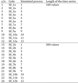
Table 7. Simulation experiments of the present study. The simulated processes are presented in Table 2.
s/n Code Simulated process Length of the time series
1 SE_1a 1 100 values
2 SE_2a 2 3 SE_3a 3 4 SE_4a 4 5 SE_5a 5 6 SE_6a 6 7 SE_7a 7 8 SE_8a 8 9 SE_9a 9 10 SE_10a 10 11 SE_11a 11 12 SE_12a 12
13 SE_1b 1 300 values
15
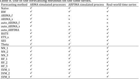
Table 8. Use of the forecasting methods on the time series.
Forecasting method ARMA simulated processes ARFIMA simulated process Real-world time series
Naïve
RW
ARIMA_f × ×
ARIMA_s × ×
auto_ARIMA_f × ×
auto_ARIMA_s × ×
auto_ARFIMA ×
BATS
ETS_s
SES
Theta
NN_1
NN_2
NN_3
RF_1
RF_2
RF_3
SVM_1
SVM_2
SVM_3
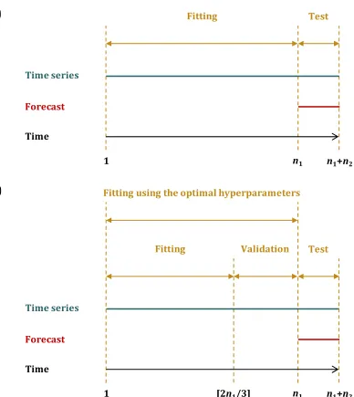
For the application of the stochastic methods we divide each time series into two
segments, i.e. the fitting segment and the test segment, which contain n1 and n2 values
respectively, as indicated in Figure 2(a). We fit the stochastic models to the former and make predictions corresponding to the latter using the recursive multi-step ahead
forecasting method. For the total of the conducted experiments n2 equals 10. For the
application of the ML forecasting methods, we additionally divide the segment of n1 values into two segments, i.e. the fitting segment (first [2n1/3] values of the time series) and the
16 (a)
(b)
Figure 2. Division of a time series into (a) two segments for the application of the stochastic methods and (b) three segments for the application of the ML methods. We note that for the latter category the validation set serves the hyperparameter optimization procedure, while both the fitting and validation segments are used to re-fit the optimum models (i.e. the models with the optimal hyperparameters) before forecasting the values of the test segment.
The validation segment serves the hyperparameter optimization procedure, as
explained subsequently. We use the fitting segment to fit several ML models that differ
only as it comes to the values of a specific hyperparameter. We use each of those models to make predictions corresponding to the validation segment and measure the RMSE of
those predictions. Finally, we decide on the value of the hyperparameter, i.e. the
corresponding to the model with the smallest RMSE on the validation segment (optimum
Forecast
Time series
Time
Fitting
1 n1+n2
Test
n1
Forecast
Time series
Time
Fitting Validation
1 [2n1/3] n1+n2
Test
n1
17
model). We fit a model with the selected hyperparameter value to data of both the fitting and validation segments and make predictions corresponding to the test segment.
Finally, we compute the values of the metrics presented in Section 2.4 for each
forecasting test. The computation takes place on the test segment, which functions as a
reference for the comparative assessment of the forecasting methods’ performance. We use the metric values for the comparative assessment of the forecasting methods, mainly
their medians and iqr values computed for each method per experiment. We compare the
medians within each experiment, as described in Table 6, while the smallest the iqr the better the forecasts. In particular, for the real-world experiment we rank the forecasting
methods for each individual test and further compute an average-case ranking for each of
the metrics. We emphasize in the 18 average-case rankings and not directly in the mean or median values of the metrics (as in Tyralis and Papacharalampous 2017), because the
latter might be more affected by the results of specific time series.
Although our computational experiments are designed to produce new knowledge in
the field of hydrological time series forecasting, there are several outcomes rather well known at the forefront of our methodological framework. In more detail, the ARIMA_f and
also the auto_ARIMA_f forecasting methods are expected to have the best performance
regarding the Type 1 accuracy, mainly in terms of RMSE, on the time series resulting from the simulation of ARMA processes because of their theoretical background (for details see
Wei 2006, pp. 88-93). Likewise, this applies to the performance of ARIMA_s and
auto_ARIMA_s regarding the capture of the variance exhibited by the time series within the same simulation experiments. Furthermore, the ARIMA_f and ARIMA_s forecasting
methods share an additional advantage, since they use by design the p, d, q numbers used
in the simulation process. Similarly to the ARIMA_f and auto_ARIMA_f forecasting methods, auto_ARFIMA is expected to be the best in terms of RMSE on the time series
resulting from the simulation of ARFIMA processes. The five forecasting methods
mentioned in the present paragraph, together with the two simple methods, play the role of benchmarks within our methodological approach, while simulation experiments are, in
general, the only available way to incorporate benchmarking into a methodological
18
3.
Results
3.1
Simulation experiments
Section 3.1 aims at providing a synopsis of the results of the simulation experiments. To
support our key findings, here we present a small representative sample of the entire
information. For the about 13 000 figures, conducted in the context of an exploratory visualization, as well as for the numerical summaries of the results in table form, the
reader is referred to the fully reproducible reports, which are available together with their codes in the supplementary material. In the latter we also enclose the report entitled
“Selected figures for the qualitative comparison of the forecasting methods”, which
includes Figures S.1-S.24. These figures can support the main conclusions of this paper in a satisfactory manner.
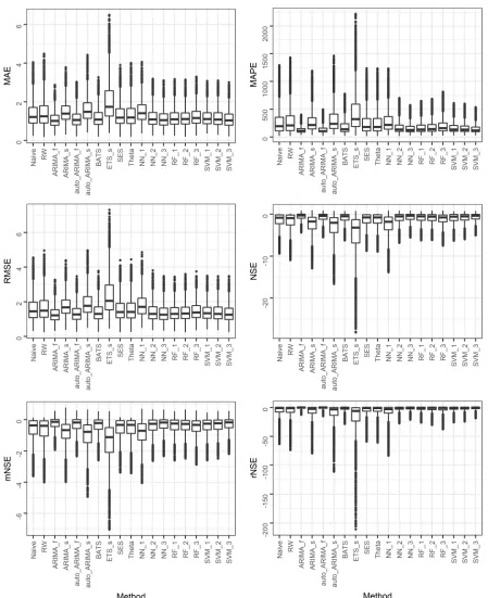
In Figures 3-5 we present the side-by-side boxplots of the metric values computed within the SE_1a simulation experiment. These figures can provide a rough outline of the
forecasting methods and the utility of the metrics within this study. By their examination,
we observe that the ARIMA_f and auto_ARIMA_f benchmarks are the best performing with respect to Type 1 accuracy, as assumed in Section 2.5, while BATS exhibits a very close to
these methods performance, perhaps because it uses information from an ARMA model.
We also note that the total of the ML methods except for NN_1 are competitive with BATS and with each other, while they are also better than the stochastic SES and Theta. The
latter forecasting methods share a quite similar performance, a fact also applying to Naïve and RW. These simple benchmarks are better than NN_1 and the simulation models
(ARIMA_s, auto_ARIMA_s, ETS_s), amongst which ETS_s produces forecasts with the most
varying metric values and the worst median. Regarding the Type 2 accuracy, all the methods seem to have rather equally good average-case performance, since the
differences in the latter are small and not perceivable from these figures. However, the
metric values computed for ETS_s are the most scattered with respect to each other, while the opposite applies to the metric values computed for ARIMA_f, auto_ARIMA_f, BATS and
all the ML methods apart from NN_1. The metric values computed for the remaining
forecasting methods are scattered with respect to each other to an extent in between.
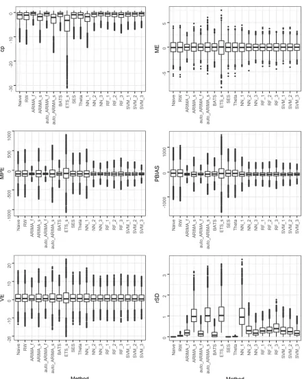
In terms of rSD, the image is rather reversed compared to the one produced by the
19
auto_ARIMA_f and ETS_s is good. Nevertheless, the rSD values for these four forecasting methods can vary significantly from the one forecasting attempt to the other, more than
the rSD values computed for the remaining forecasting methods, a fact also applying to the rest of the metrics. Regarding the average-case performance with respect to
correlation, ARIMA_f, auto_ARIMA_f and BATS are the best, followed by NN_3. With
respect to Type 1 accuracy and capture of the variance, ARIMA_f, auto_ARIMA_f, BATS and
all the ML methods apart from NN_1 are clearly better than the simple benchmarks and competitive with each other. SES and Theta, on the other hand, exhibit a very close
performance to the one of Naïve and RW. Finally, in terms of KGE, the best performing
methods are the same three stochastic and eight ML ones. NN_1, ARIMA_f and auto_ARIMA_f are better than Theta, which is competitive with RW. Overall, we observe
that for the SE_1a simulation experiment the metrics (even the corresponding to the same criterion) provide different aspects of the same information to an extent larger or smaller,
while these 18 different aspects may also be conflicting to each other.
Subsequently, we state the main observations obtained from the total of the simulation
experiments. To base these observations, in Figure 6 we present the heatmaps of the
average-case performance of the forecasting methods within the SE_1a, SE_1b, SE_2a and SE_2b simulation experiments, while in Figures 7-9 we present the heatmaps formed
using the medians of the total of the RMSE, rSD and d metric values respectively. In these
figures the scaling is performed in the row direction and the darker the colour the better the forecasts. A clustering analysis on the forecasting methods based on their
performance is also applied. Some observations obtained from SE_1a apply to the rest of
the simulation experiments as well. These are the following (see, for example, Figures 6-9): (a) forecasting methods from both the stochastic and ML categories are amongst the
best performing and the worst performing ones, (b) the metrics can provide significantly different, even conflicting, image regarding the performance of the forecasting methods,
(c) the ARIMA_f, auto_ARIMA_f and auto_ARFIMA benchmarks are the best performing in
terms of Type 1 accuracy, while ETS_s, and the ARIMA_f and auto_ARIMA_f benchmarks exhibit a good average-case performance in terms of rSD, (d) the image produced by rSD
is reversed with respect to the one produced by the Type 1 accuracy metrics, i.e. the well
performing with respect to the latter criterion are bad performing with respect to the capture of the variance of the time series, (e) BATS is very close to the ARIMA_f,
20
Theta, exhibit similar performance with each other. Nevertheless, the Pr, r2 and KGE values computed for Naïve and SES are infinite. Finally, by the examination of the
side-by-side boxplots produced for each and every of the simulation experiments we note that (g) the ARIMA_s, auto_ARIMA_s, ETS_s and NN_1 forecasting methods seem to share a form
of instability, i.e. their metric values vary more with each other than the metric values of
other forecasting methods. The latter concerns the results obtained from all the metrics
21
22
23
24
(a) (b)
(c) (d)
25
26
27
Figure 9. Heatmaps for the comparative assessment of the forecasting methods according to the median values of the d metric and the condition stated on Table 6.
By the examination of Figure 6 (or Figures S.1-S.6) we observe that the image provided
by the metrics and the resulted clustering of the forecasting methods can also vary from the one simulation experiment to the other, while by the examination of Figures 7-9 (or
28
provided by specific metrics or due to specific forecasting methods. In fact, the heatmaps formed for the MAE, MAPE, RMSE, NSE, mNSE, rNSE, cp and KGE are smoother than those
formed for the remaining metrics. In particular, the pictures obtained from the ME, MPE, VE, r2, d and md metrics are the most dispersed. On the other hand, the Naïve, RW,
ARIMA_s, auto_ARIMA_s, ETS_s, SES, Theta and NN_1 forecasting methods are more likely
to have a varying performance. For example, we observe that Naïve and RW exhibit rather
the best average-case performance in terms of d (see Figure 9) and md (see Figure S.22), while they have either bad, moderate or good average-case performance in terms of MAE,
MAPE, PBIAS and VE depending on the simulation experiment (see Figures S.7, S.8, S.16
and S.17 respectively). The same applies to SES and Theta in terms of d, etc. We also note that forecasting methods resulting from the implementation of the same algorithm can
exhibit a far distant or always close performance depending on the algorithm. For instance, NN_1 and NN_2 (or NN_3) may differ with each other to a great extent, a fact also
applying to ARIMA_s and ARIMA_f, but not to the RF and SVM forecasting methods.
Regarding NN_1, we observe that length of the time series largely affects its performance in a systematic way, while the performance of the rest forecasting methods is less or even
slightly affected. The latter effect depends on the forecasting method, as well as on the
simulated process. In detail, the NN_1 forecasting method exhibits a bad performance with respect to Type 1 accuracy (and a good one in terms of rSD; see Figure 8), when
applied to the time series of 100 values, while its performance becomes good with respect
to Type 1 accuracy (and bad in terms of rSD), when applied to the time series of 300 values. The latter observation might apply to a small extent to some of the remaining ML
methods.
Finally, we summarize some important information about the best performing
forecasting methods in terms of Type 1 accuracy. A good performance with respect to this criterion is a major pursuance in most of the forecasting applications. In terms of MAE
(see Figure S.7) BATS is very close to the ARIMA_f, auto_ARIMA_f and auto_ARFIMA
benchmarks, while SES, Theta and all the ML methods except for NN_1 have always a good or moderate performance. With respect to the MAPE metric (see Figure S.8) SVM_3 and
BATS are mostly close to ARIMA_f, auto_ARIMA_f and auto_ARFIMA, and NN_2, NN_3,
RF_1, RF_2, RF_3, SVM_1, SVM_2, SVM_3, SES and Theta are well performing for the greatest part of the simulation experiments. The same observations apply with respect to
29
benchmarks as well. Regarding the NSE, mNSE, rNSE and cp values (see Figures S.10, S.11, S.12 and S.13 respectively), most of the stochastic and ML methods are competitive to
each other and to the good benchmarks. The only ones that are not competitive are the simulation models, the simple benchmarks and NN_1, the latter when applied to time
series of 100 values.
3.2
Real-world experiment
In full correspondence to the simulation experiments, the results of the real-word
experiment are presented in both quantitative and qualitative forms. In Figure 10 we present the side-by-side boxplots of the MAPE, NSE, cp, MPE, d and KGE values.
Additionally, in Table 9 we present the median values of the dimensionless metrics, while
in Figure 11 the average-case rankings of the forecasting methods. Here as well, we observe small differences between most of the methods, especially with respect to specific
metrics (e.g. MAPE, cp, MPE, d). For example, the median values of MAPE computed for
auto_ARFIMA, BATS, SES, Theta, NN_3, RF_1, SVM_1, SVM_2 and SVM_3 are very close to each other. The same applies to the median values of NSE computed for the same methods,
although the differences in the respective side-by-side boxplots seem to be larger in the
latter case than in the former. Because of the small differences in the performance of the forecasting methods, the median metric values of Table 9 (e.g. the median MAPE values)
may result to a different ranking of the forecasting methods than the average-case ranking
presented in Figure 11. We note that values of NSE, most of which are lower than 0 (see Table 9 and Figure 10), should not be surprising, since the examined problem differs from
the traditional rainfall-runoff problem. In the latter exogenous variables are incorporated
with significant increase in the available information (see also the discussion in Section 4).
Furthermore, while the average-case rankings with respect to accuracy mostly favour
stochastic methods (SES, Theta, auto_ARFIMA and BATS), SVM_1 is also ranked amongst
the best performing methods. In more detail, SES is ranked first according to MAE, RMSE, NSE, mNSE, cp, ME, MPE, PBIAS and VE, but it is worse than SVM_1 and SVM_2, and SVM_1,
SVM_2 and SVM_3 according to MAPE and rNSE respectively. With respect to the latter
metrics, the best performing method is BATS. This method has a rather moderate overall performance in terms of accuracy. The less accurate methods, on the other hand, are
30
respect to the remaining criteria, SES is clearly the worst performing method, while Theta, Naïve, BATS, SVM_1, NN_3 and auto_ARFIMA are also ranked behind the remaining ML
methods, amongst which NN_1 is mostly ranked first.
31
Table 9. Median values of the dimensionless metrics computed within the real-word experiment. N aï ve R W au to _A R F IM A B A T S E T S_ s SE S T h et a N N _1 N N _2 N N _3 R F _1 R F _2 R F _3 SV M _1 SV M _2 SV M _3
MAPE 29.21 29.83 22.04 22.04 33.54 22.02 22.83 32.30 24.05 22.95 22.80 25.39 25.17 22.06 22.46 22.15 NSE -0.72 -0.84 -0.20 -0.19 -1.53 -0.17 -0.18 -1.26 -0.33 -0.22 -0.26 -0.46 -0.48 -0.22 -0.25 -0.26 mNSE -0.27 -0.31 -0.07 -0.07 -0.59 -0.06 -0.07 -0.51 -0.14 -0.09 -0.12 -0.21 -0.22 -0.07 -0.10 -0.11 rNSE -0.81 -0.90 -0.35 -0.39 -2.18 -0.35 -0.45 -1.83 -0.59 -0.45 -0.45 -0.84 -0.82 -0.37 -0.39 -0.38 cp 0.09 0.03 0.39 0.38 -0.33 0.39 0.38 -0.16 0.30 0.36 0.37 0.27 0.24 0.38 0.32 0.33 MPE 2.83 1.47 2.99 2.20 4.54 3.32 5.07 2.94 4.61 3.36 4.34 3.81 3.61 2.51 1.25 0.41 PBIAS -6.34 -6.34 -3.14 -4.25 -2.78 -2.86 -1.67 -3.05 -2.09 -2.41 -1.27 -2.50 -3.04 -3.89 -5.41 -5.88 VE 0.71 0.71 0.78 0.78 0.68 0.78 0.78 0.69 0.76 0.78 0.78 0.75 0.76 0.78 0.77 0.78 rSD 0.00 0.03 0.05 0.00 1.00 0.00 0.01 0.94 0.21 0.05 0.24 0.44 0.41 0.00 0.13 0.08 Pr ∞ -0.05 0.06 0.04 0.00 ∞ -0.04 0.08 0.08 0.02 0.07 0.07 -0.01 0.10 0.04 0.05 r2 ∞ 0.07 0.06 0.05 0.06 ∞ 0.07 0.05 0.06 0.06 0.06 0.07 0.06 0.07 0.07 0.07 d 0.41 0.41 0.39 0.36 0.38 0.36 0.36 0.40 0.39 0.37 0.39 0.39 0.38 0.39 0.39 0.39 md 0.31 0.31 0.28 0.28 0.29 0.27 0.26 0.30 0.29 0.28 0.28 0.30 0.30 0.29 0.30 0.29 rd 0.29 0.30 0.25 0.26 0.29 0.22 0.18 0.33 0.28 0.22 0.28 0.29 0.32 0.29 0.34 0.36 KGE ∞ -0.47 -0.35 -0.34 -0.16 ∞ -0.46 -0.12 -0.24 -0.35 -0.23 -0.17 -0.20 -0.32 -0.29 -0.32
32
4.
Discussion
4.1
Contribution in hydrology and beyond
The present study contributes by developing a detailed framework for assessing
forecasting techniques in hydrology. Furthermore, its findings can provide new insights
into the nature of short hydrological time series forecasting, while they concern all natural processes that could be modelled by stationary processes and all possible time scales. A
first view of the results suggests that the differences in the performance of the forecasting methods are mostly small (insignificant for hydrometeorological applications), while the
stochastic and ML methods can share a quite similar performance when forecasting
hydrological time series of small length. In fact, methods from both these categories are found to perform better or worse mainly depending on the metric, but on the experiment
as well. Regarding the Type 1 accuracy, in the simulation experiments BATS is always
close to the ARIMA_f, auto_ARIMA_f and auto_ARFIMA benchmarks, probably because it uses information from an ARMA model, while most of the ML methods (e.g. NN_3 and
SVM_3) are amongst the best performing and often better than SES and Theta.
Nevertheless, in the real-world experiment SES is mostly ranked first, followed by auto_ARFIMA, BATS, SVM_1 and Theta, while NN_3, RF_1, SVM_2, and SVM_3 are also close
to the latter methods. This outcome might mean that for a different sample of river
discharge time series, the average-case rankings would differ as well, and that there might be no particular reason to choose some methods over others for this specific process.
Given the claims that in linear situations (e.g. the simulation experiments of this study)
the ML methods are more likely to be inferior to the stochastic ones, while in non-linear situations, as it could apply to river discharge processes, the ML methods are more likely
to outperform, the algorithmically obtained results of the present study are even more
interesting. Noteworthy is also the fact that our results differ from the results of Makridakis et al. (2018), which favour the stochastic methods, probably due to the
different experimental settings.
In this view, we would like to emphasize that the ML algorithms are accurate enough,
while a worth-mentioning particularity of theirs is perhaps related to the concomitant to the use of many lagged variables decrease of the fitting set (for more details, see Tyralis
and Papacharalampous (2017)) and is largely perceivable through the examination of the
33
100 values, NN_1 exhibits a bad performance in terms of Type 1 accuracy (a fact not applying to NN_2 and NN_3, which use less and very few lagged variables respectively).
On the contrary, for the simulation experiments using time series of 300 values, this method is amongst the most accurate ones. The same number of lagged variables is used
by RF_1 and SVM_1. Nevertheless, the performance of the RF and SVM algorithms seems
to be less affected by the length of the fitting set. In fact, (lagged) variable selection may
significantly affect the performance of a ML algorithm (see, for example, the regression case study of Anctil et al. (2009)); therefore, it is the objective of many studies (e.g. Kohavi
and John GH (1997), Tyralis and Papacharalampous (2017)).
While there are forecasting methods regularly better or worse than others with respect
to specific criteria, this does not apply to all the forecasting methods neither to all the criteria. For example, we observe that Theta can exhibit good, moderate or bad
average-case performance in terms of specific metrics depending on the simulation experiment.
Furthermore, sophisticated forecasting methods (such us the above mentioned ones) do not necessarily (but mostly) provide better forecasts than the simple Naïve and RW, as
also shown in previous studies (e.g. Makridakis and Hibon (2000), Cheng et al. (2017)).
These two methods perform almost identically in the experiments of the present study, but not for longer forecast horizons (see Papacharalampous et al. (2017b; 2018c)).
Another pair of similarly performing forecasting methods is SES and Theta, as proved in
Hyndman and Billah (2003).
In general, we cannot decide on a universally best or worst forecasting method (stochastic or ML), neither we can rank the forecasting methods based on the results of
the simulation experiments. Even the relative metrics, i.e. the corresponding to the same
criterion (see Table 6), provide measurements which lead us to different aspects of the same information to an extent larger or smaller depending on the pair of metrics
considered. Some of these 18 different aspects are also conflicting to each other. Any
ranking of the forecasting methods would require the a priori selection of an experiment and a criterion of interest, as well as the application of a simplification procedure (e.g. use
of the median values of the selected metric) and, thus, would not be general. However, the
classification of the forecasting methods is possible, though only to some extent. This classification could be based on the similar or contrasting performance of the forecasting
34
respect to the capture of the variance, while they are clearly the worst performing in terms of Type 1 accuracy. This happens, since these two criteria are contradictory. For
instance, the optimum forecast for an ARFIMA model is obtained when the innovations are set to be zero.
Our contribution in the field of hydrology also includes the implementation of several forecasting models barely used in hydrometeorological concepts, but commonly used in
the forecasting field (RW, BATS, ETS, SES and Theta) or for regression purposes (RF). This
innovation holds, especially if we could exclude from the hydrological literature the large-scale companions of this study, i.e. Papacharalampous et al. (2017b; 2018b,c) and Tyralis
and Papacharalampous (2017), while its practical value is indisputable. One could claim
that there may be an undiscovered forecasting method (stochastic or ML), which will be better than the existing ones. As regards the “myth of the best method” the reader is
referred to Hong and Fan (2016), who mention that the number of original techniques is
countable and has been exhausted, while the hybrid techniques, i.e. combinations of original techniques, cannot improve further the forecasting performance.
Another important contribution of the present study is related to the so-called “no free
lunch theorem” (Wolpert 1996). According to Wolpert (1996), in the space of all possible
problem instances, there is not a model, which will always perform better than the other models, in the absence of significant information for the problem at hand. The present
empirical study shows that even in the finite space of simple (simulated) and real-world
time series examined here there is not an optimal forecasting solution. Finding the best algorithm mostly depends on our knowledge of the system. For example, using ARFIMA
models for forecasting the ARFIMA simulated time series is obviously the best choice, due
to the prior known information about the system. The other methods are equivalent in performance since they cannot incorporate this knowledge. In the specific class of
hydrological processes forecasting finding information about the examined system could
be possible, e.g. with the application of principles of physics, such as the maximum entropy principle, incorporation of information from deterministic models (e.g. Tyralis
and Koutsoyiannis 2017), understanding the processes from a chaotic perspective
(Sivakumar 2004) and other approaches. Obviously, the knowledge of the system is not simply equivalent to the knowledge of its statistical properties, e.g. the mean, variance,
35
the literature of the hydrological science blind use of forecasting methods is not suggested.
Additionally, it seems that major advancements in the time series forecasting
performance of all methods can be achieved by incorporating appropriate exogenous
variables in the model, while the potential for improving their performance in univariate time series forecasting seems limited. The latter in our opinion is also due to the nature
of the problem, which is simple. Therefore, methods that are more complicated will not
necessarily yield better results. A similar example is for instance the difference in the games of tic-tac-toe and Go. The former game is simple and can be solved by simple
algorithms, therefore the choice of the method is not of relevance. On the other hand, the
best performance on the more complex game of Go was achieved by the use of complicated machine learning algorithms (e.g. Silver et al. (2016)).
Regarding the extent to which the conclusions could be generalizable for the
forecasting of short hydrological time series, we note that the stationarity assumption and
the reasoning concerning its appropriateness in the modelling of geophysical properties in Koutsoyiannis and Montanari (2015) is consistent with the no free lunch theorem. In
particular, if we cannot explain the behaviour of a geophysical process based on a
deterministic mechanism, then the most appropriate models are stationary. Even in cases of deterministic systems, stochastic approaches are appropriate (Koutsoyiannis 2010).
This is a frequently met case in modelling of geophysical processes (i.e. there is not an
adequate explanation for the behaviour of the geophysical process), proving that our conclusions could be generalizable. Finally, in practical terms the contribution of this
study can be summarized as follows. A forecasting problem should be approached with
more than one algorithmic solutions, i.e. using many forecasting methods (stochastic and ML), while the final judgment should always be provided by an expert.
4.2
On the methodological approach
The above section highlights the efficiency of our methodological approach in producing
large-scale and representative for the field of hydrology results. Moreover, the real-world experiment particularly accounts for the case of river discharge forecasting. Someone
who examines both the results of the simulation experiments and the real-world
experiment has a more complete picture of the underlying phenomena than whom
36
simulated processes combined with benchmarking has proved pivotal in achieving our aim under the stationarity assumption. Additionally, the use of an adequate number of
forecasting methods and metrics in the present study is also of crucial importance. Using fewer forecasting methods and fewer metrics would have led to a very different overall
picture, particularly if those fewer metrics corresponded to fewer criteria. Besides, the
comparison is rather the only available research method for any evaluation and,
consequently, the larger its scale the more generalized the derived results. For this specific reason, the novel (mainly with respect to hydrology) methodological approach of
the present study is considered appropriate for the assessment of forecasting methods in
hydrology. Furthermore, the qualitative form of the results facilitates their handy examination and, thus, eases the delivery of the large-scale findings. In fact, our
methodology enables the assessment of the failure risk or, alternatively worded, the available opportunities for success that accompany the use of a specific forecasting
method to a significant extent, while it also leads to the recognition of several
advantages/disadvantages characterizing the latter. This knowledge is fundamental to the forecasters and the users of the forecasts, since a specific forecasting method can be
both useful and useless, depending on the forecasting task.
5.
Conclusions
We conduct an extensive comparison between several stochastic and machine learning
methods for the multi-step ahead forecasting of hydrological processes by performing large-scale computational experiments based on simulations under the stationarity
assumption. The implemented stochastic methods include simple models, models from
the frequently used families of Autoregressive Moving Average and Autoregressive Fractionally Integrated Moving Average, as well as State Space and Exponential
Smoothing models, while the machine learning ones are Neural Networks, Random
Forests and Support Vector Machines. The aim is to provide large-scale results, while the respective comparisons in the literature are usually based on case studies. We also run a
real-world experiment on the largest river discharge dataset ever used for forecasting purposes. Despite this specific focus, the results concern all natural processes that could
be modelled by stationary processes and all possible time scales. The findings suggest that
stochastic and machine learning methods do not differ dramatically. In fact, methods from
37
forecasting. This is particularly important, because it reveals that the forecast quality is subject to certain limitations. It is also consistent with the no free lunch theorem, albeit
the theorem refers to an infinite space of problems instances, while here we examined a finite space of problems. The empirical investigation showed that in the given finite space,
formed by simulated and annual river discharge time series, it is still satisfied. The
practical conclusion drawn from this paper is that, unless there is relevant theoretical
knowledge, a forecasting problem should be algorithmically approached using many forecasting methods (stochastic and machine learning), while the final judgment should
be made by an expert.
Acknowledgements: Part of the Discussion section (in particular the comments on the no free lunch theorem and the use of exogenous variables) has been inspired by the
“Energy Forecasting” blog (http://blog.drhongtao.com/).
Funding: This research did not receive any specific grant from funding agencies in the public, commercial, or not-for-profit sectors.
Declarations of interest: none
Author contributions: HT conceived the idea of comparing stochastic vs machine learning methods in hydrological univariate time series forecasting using large datasets.
GP designed the experiments, performed the computations and wrote the manuscript under the supervision of HT during her MSc thesis. All authors have discussed the results
and edited the manuscript.
Appendix A Statistical software and supplementary material
The analyses and visualizations have been performed in R Programming Language (R
Core Team 2017). We have used the contributed R packages cgwtools (Witthoft 2015),
devtools (Wickham and Chang 2017), EnvStats (Millard 2013), forecast (Hyndman and Khandakar 2008; Hyndman et al. 2017), fracdiff(Fraley et al. 2012), gdata (Warnes et al.
2017), ggplot2 (Wickham 2016), HKprocess (Tyralis 2016), kernlab (Karatzoglou et al.
2004), knitr (Xie 2014, 2015, 2017), nnet (Venables and Ripley 2002), randomForest (Liaw and Wiener 2002), readr (Wickham et al. 2017), rminer (Cortez 2010, 2016) and
38
The supplementary material is available in Papacharalampous et al. (2018a). We provide the fully reproducible reports together with their codes. We also provide the
reports entitled “Definition of the stochastic processes’’, “Definition of the metrics’’, “Selected figures for the qualitative comparison of the forecasting methods’’, which we
suggest to be read alongside with Sections 2.1, 2.4 and 3.1 respectively.
References
Abrahart RJ, Anctil F, Coulibaly P, Dawson CW, Mount NJ, See LM, Shamseldin AY, Solomatine DP, Toth E, Wilby RL (2012) Two decades of anarchy? Emerging themes and outstanding challenges for neural network river forecasting. Progress in Physical Geography 36(4):480–513. doi:10.1177/0309133312444943
Abudu S, Cui C, King JP, Abudukadeer K (2010) Comparison of performance of statistical models in forecasting monthly streamflow of Kizil River, China. Water Science and Engineering 3(3):269–281. doi:10.3882/j.issn.1674-2370.2010.03.003
Ahmed NK, Atiya AF, GayarAn NE, El-Shishiny H (2010) An empirical comparison of machine learning models for time series forecasting. Econometric Reviews 29(5– 6):594–621. doi:10.1080/07474938.2010.481556
Alpaydin E (2010) Introduction to Machine Learning, second edition. MIT Press
Anctil F, Filion M, Tournebize J (2009) A neural network experiment on the simulation of daily nitrate-nitrogen and suspended sediment fluxes from a small agricultural
catchment. Ecological Modelling 220(6):879–887.
doi:10.1016/j.ecolmodel.2008.12.021
Assimakopoulos V, Nikolopoulos K (2000) The theta model: a decomposition approach to forecasting. International Journal of Forecasting 16(4):521–530. doi:10.1016/S0169-2070(00)00066-2
Atiya AF, El-Shoura SM, Shaheen SI, El-Sherif MS (1999) A comparison between neural-network forecasting techniques-case study: river flow forecasting. IEEE Transactions on Neural Networks 10(2):402–409. doi:10.1109/72.750569
Ballini R, Soares S, Andrade MG (2001) Multi-step-ahead monthly streamflow forecasting by a neurofuzzy network model. IFSA World Congress and 20th NAFIPS International Conference:992–997. doi:10.1109/NAFIPS.2001.944740
Bontempi G (2013) Machine Learning Strategies for Time Series Prediction. European Business Intelligence Summer School, Hammamet, Lecture. 2013. Available online: https://pdfs.semanticscholar.org/f8ad/a97c142b0a2b1bfe20d8317ef58527ee329 a.pdf (accessed on 14 October 2017)
Box GEP, Jenkins GM (1968) Some recent advances in forecasting and control. Journal of the Royal Statistical Society. Series C (Applied Statistics) 17(2):91–109. doi:10.2307/2985674
Breiman L (2001a) Random Forests. Machine Learning 45(1):5–32.
doi:10.1023/A:1010933404324
Breiman L (2001b) Statistical modeling: The two cultures (with comments and a rejoinder by the author). Statistical Science 16(3):199–231