Extended evolutionary structural optimization method for multi-storey buildings

(1)

(2)

DECLARATION

D E C L A R A T I O N

I, Dang Quang NGUYEN, hereby declare that the materials embodied in this

thesis have not been submitted in part or full to any other university or institute

for award of any degree.

__2.

(3)

(4)

SUMMARY

SUMMARY

This study extends the Evolutionary Structural Optimization (ESO) method for application to multi-storey buildings. T h e objective is to find the optimal topologies of multi-storey buildings subject to overall stiffness or displacement constraints. It emphasizes the derivation of a methodology to help the structural designers to choose the optimal topology a m o n g m a n y topologies that are generated during the evolutionary optimization process. Other problems of the E S O method such as the termination condition, sharp change in structural m e a n compliance or constrained displacements are also investigated.

The new added features provide the ESO method with the capability of dealing with structures containing different types of finite elements. For the structure being considered, only continuum elements are allowed to be removed during the optimization process while b e a m elements are assumed to be fixed and are referred to as a non-design domain. B y having all the topologies with the same weight as the initial structure, the performance of these topologies can be evaluated b y comparing the m e a n compliance or constrained displacements. The results of this study show the extended ESO method can effectively find

(5)

A C K N O W L E D G E M E N T S

I would like to thank Professor Mike Xie for providing inspiration and guidance throughout the project. His endless effort, encouragement and enthusiasm have been instrumental in helping me overcome the many

challenges faced during this research. Without his valuable guidance this thesis would not have been possible.

I would like to thank my Mum and Dad who have always been there when

needed, as well as being fantastic and loving parents. Special thanks to my uncles Khanh NGUYEN, Kha NGUYEN and their families for their

encouragement and hospitality during the time I have been in Melbourne,

Australia. I am also greatly in debt to my uncle Lap and his family for their invaluable advice and English correction.

I would also like to take this opportunity to express my thanks to:

• School of the Built Environment, Victoria University of Technology, which provided facilities for this research.

(6)

A CKNO WLEDGEMENTS

(7)

C O N T E N T S

Declaration i

Summary ii

Acknowledgements iii

Contents v

CHAPTER 1: INTRODUCTION

1.1 Structural Optimization 1

1.2 A i m s of Research 4

1.3 Significance of the Research 5

1.4 Layout of Thesis 5

CHAPTER 2: LITERATURE REVIEW

2.1 Definitions 8

2.2 Classical Methods in Structural Optimization 11

2.3 Modern Methods in Structural Optimization 13

2.3.1. Mathematical Programming Methods ( M P methods) 13

2.3.2. OptimalitvCriteria Methods ( O C methods) 16

2.3.3. Genetic Algorithm Method ( G A method) 20

2.3.4. Homogenization Method 23

2.3.5. Evolutionary Structural Optimization Method ( E S O method) 26

2.4 C o m m e n t s on Current Research and Applications 31

CHAPTER 3: THE EXTENDED ESO METHOD FOR OVERALL

STIFFNESS CONSTRAINT

3.1 Introduction 33

3.2 Optimization Problem Statement 33

3.3 Element Removal Criteria Based on Strain Energy Density 35

(8)

CONTENTS

3.5 Uniformly Changing the Thickness of Continuum Elements 38

3.6 Termination Conditions 43

3.7 Handling Sharp Change in the M e a n Compliance Values 44

3.8 Design Procedure 47

3.9 Examples 51

3.9.1. A Plane Stress Structure (Two-bar Frame) 51

3.9.2. A Plate in Bending 55

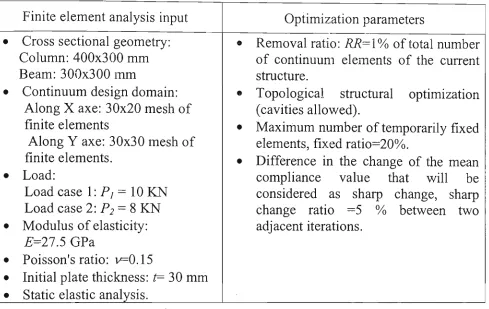
3.9.3. A 3 D Structure Containing B earn and Continuum Elements 59

3.10 S u m m a r y 66

CHAPTER 4: THE EXTENDED ESO METHOD FOR MULTI-STOREY

BUILDINGS SUBJECT TO OVERALL STIFFNESS CONSTRAINT

4.1 Introduction 68

4.2 Structural Optimization Problem 70

4.3 Optimization Procedure 71

4.4 Example 76

4.5 S u m m a r y 84

CHAPTER 5: THE EXTENDED ESO METHOD FOR DISPLACEMENT

CONSTRAINTS

5.1 Introduction 86

5.2 Optimization Problem Statement 87

5.3 Element Removal Criterion Based on Virtual Strain Energy Density.. 88

5.4 Structures Under Multiple Load Cases 90

5.5 Uniformly Changing the Thickness of Continuum Elements 91

5.6 Termination Conditions 92

5.7 Handling Sharp Change in the Constrained Displacement(s) 92

5.8 Design Procedure 93

5.9 Examples 97

5.9.1. A Plane Stress Structure 97

(9)

CHAPTER 6: THE EXTENDED ESO METHOD FOR MULTI-STOREY

FRAME BUILDINGS SUBJECT TO TOP DEFLECTION

CONSTRAINTS

6.1 Introduction 114

6.2 Optimization Procedure 115

6.3 2D Plane Stress Multi-Storey Steel Frame 119

6.4 Summary 125

CHAPTER 7: CONCLUSIONS AND RECOMMENDATIONS

7.1 Conclusions 126

7.2 Limitations of This Research 127

7.3 Recommendations for Further Research 129

(10)

CHAPTER /• INTRODUCTION

C H A P T E R 1: INTRODUCTION

1.1 STRUCTURAL OPTIMIZATION

Structural optimization aims to find the best design for a loaded structure which

has the minimum weight or cost, while satisfying the requirements of strength,

stiffness, stability and functionality. It is motivated by the growing realization

of the scarcity of natural resources. In general, it is desirable that every design

should be optimized. For example, a car must be designed such that minimum

fuel consumption is achieved while maintaining the highest performance, an

aeroplane is designed in such a way that it costs the least for material or capital

while it maintains good in-flight performance during its lifetime. Structural

optimization can be divided into three main categories, namely, size, shape and

topological optimization. Among them, topological structural optimization is

considered the most challenging because the topology and shape of the

structure are both changed during the optimization process. Topological

structural optimization will seek the pattern or the configuration of structural

components which form an optimal structure.

In the building industry, the task of integrating structural optimization into a

building design is an issue of significant concern. A typical building structure

contains columns, beams and shear-walls. The sizes and locations of these

elements need to be determined during the design process. Because of the

(11)

The evolutionary structural optimization (ESO) method introduced by Xie and Steven (1997) effectively bridges the gap between Finite Element Analysis ( F E A ) and structural optimization. In the E S O method, the structural optimization is carried out in an iterative manner based o n the simple idea of systematically removing inefficient elements, with the result that the residual structure evolves toward an optimum. Currently, the E S O method has been developed to solve those structural optimization problems which are subject to overall stiffness, displacement, frequency and buckling constraints.

(12)

CHAPTER I- INTRODUCTION

carrying mechanism of two-dimensional (2D) structures. The applicability of this method, however, is limited to 2D structures because of the basic

assumption that the global stiffness matrix is a linear function of the design variables.

The purpose of this thesis is to extend the ESO method for applications to multi-storey building structures. Weaknesses in the ESO method such as the termination conditions, the sharp changes in the constrained function values and maintenance of structural symmetry are examined. A review of current

literature identifies a lack of application of structural optimization to practical building structures, particularly to three-dimensional (3D) structures.

(13)

1.2 AIMS OF RESEARCH

The aim of the thesis is to extend the ESO method to multi-storey buildings

with stiffness and displacement constraints. The model of the building contains

a combination of beams and continuum elements under multiple cases of lateral

loading.

In order to achieve this general aim, the following specific aims are considered:

• Review the existing methods of structural optimization, their advantages,

disadvantages and difficulties when applied to solve practical problems.

Study topological optimization in detail. Particular attention will be paid to

the Evolutionary Structural Optimization (ESO) method.

• Derive an algorithm to determine the optimal topology among the whole

series of topologies generated during the evolutionary optimization process.

Based on the algorithm the termination condition of the procedure will be

derived.

• Derive an algorithm to handle sharp changes in constrained function values.

• Develop a program to carry out the structural optimization automatically.

This program will use the output data of the finite element analysis package

(14)

• Test the program on several simple topological structural optimization

problems and compare optimal topologies with previous results in the

literature.

• Apply the topological structural optimization technique to multi-storey

buildings and determine the optimal topologies subject to overall stiffness

or displacement constraints under multiple load cases.

1.3 SIGNIFICANCE OF THE RESEARCH

In this research, the ESO method is extended and is applied to multi-storey

buildings subject to overall stiffness or displacement constraints. This

extension has not been satisfactorily investigated in the discipline of structural

optimization. The outcome of this research will make a contribution to building

structural design in particular and the application of structural optimization in

general.

1.4 LAYOUT OF THESIS

This thesis consists of seven chapters:

• Chapter 2: Literature review. A review of the development and application

of structural optimization methods will be presented. Topological

(15)

Chapter 3: The extended ESO method for overall stiffness constraint. An

extended ESO method for continuum topology optimization subject to

overall stiffness constraint is developed. Concepts and definitions of the proposed method will be introduced. The issues related to the extended ESO method such as the termination condition, choosing optimal topology and sharp change in constrained function values will be addressed and handled. Several numerical examples including a 3D structure will also be presented to demonstrate the effectiveness of the method.

Chapter 4: The extended ESO method for multi-storey frame buildings

subject to overall stiffness constraint. The proposed method will be applied to a multi-storey steel frame subject to overall stiffness constraint. The structural optimization problem is to determine an efficient bracing system for the frame under multiple lateral load cases. The issue of maintaining structural symmetry will be also considered.

Chapter 5: The extended ESO method for displacement constraints. The

theoretical basis of the extended ESO method for displacement constraints will be developed. Several numerical examples will be given at the end of the chapter to verify the method.

Chapter 6: The extended ESO method for multi-storey buildings subject to

(16)

bracing system for the steel frame subject to constraint on the deflection at the top under multiple lateral load cases.

• Chapter 7: Conclusions and recommendations. Conclusions and

(17)

C H A P T E R 2: LITERATURE R E V I E W

In this chapter, a review on the development and applications of structural

optimization methods will be presented. Although this thesis focuses on

topological structural optimization, sizing and shape structural optimization

methods are also reviewed in this chapter.

2.1 DEFINITIONS

• Design variables

A structural system can be described by a set of quantities. Based on practical

experience, some quantities are chosen before the optimization process. Those

quantities are considered as pre-defined variables and they are fixed during the

optimization process. Other quantities, which are allowed to vary for

optimization purposes, are considered as design variables. From a physical

point of view, design variables can be divided into the following categories:

> Material properties: Material properties of structural elements such as

modulus of elasticity E and material density p are design variables.

> Structural topology: The patterns of connections as well as the number of

elements in the structure are design variables.

(18)

CHAPTER 2: LITERATURE REVIEW

the width of the bay in a frame building or the cross sectional dimensions of structural elements.

Depending on specific problems, design variables may be treated as discrete or continuous.

• Constraints

Every structural system has to satisfy the design requirements.

These requirements may be given by the design practice code, the availability of material, the feasibility of construction, the behaviour or other

considerations. Sets of design variables that meet all the requirements are called a feasible design. Restrictions on the design variables or the structural response are called constraints. There are two types of constraints:

> Side constraints: These constraints are imposed upon the design variables in explicit or implicit forms. Constraints such as minimum height of the beam for electrical conduit placement or minimum thickness of the plate are typical examples of side constraints.

> Behavioural constraints: These constraints are derived from the behavioural requirements of the structure. Limitations on the maximum stresses, displacements or buckling are typical examples of behavioural constraints.

(19)

D <D <D (Displacement constraints) (2.2)

where:

cr. the stress of structural members.

(j1, <ru: the lower bound and upper bound of the stress respectively.

D: the displacement of the structure.

DL, Du: the lower bound and upper bound of displacement respectively. Along with the number of design variables, the number of constraints in optimization problems has a significant impact on the time and effort of solution process. Therefore, the simplification of constraints needs to be carefully considered in order to reduce the solution effort.

Optimization problems, which have no constraints, are called unconstrained optimizations or considered as constrained optimizations otherwise.

• Objective functions

In order to evaluate the efficiency of designs, objective functions are defined and minimized during the optimization process. Objective functions may be the functions that represent the weight or the cost of the structures. The weight of the structure is the most commonly used due to the fact that it is readily

(20)

f{X) = f

d

W

l

(2-3)

/=!

where:

f(X): objective function.

W(. the weight of the i

th

element of the structures.

n: the number of total elements.

2.2 CLASSICAL METHODS IN STRUCTURAL OPTIMIZATION

The development of mathematical optimization started with the introduction of

calculus by Newton and Leibniz during the latter part of the 17 century. Given

a continuously differentiable objective function/^, the necessary condition

for the minimization off(X) atX is:

Vf = 0 (2.4)

where:

Vf: the vector of the first derivatives, or the gradient vector of the

objective function calculated atX.

F

/^(,.,./l (2.5)

\dx

x

dx

2

dx

n

\

X: the vector of the design variables.

n: the number of design variables. -„ .,, •

The sufficient condition for a local minimum of f(X) at X involves the

calculation of the matrix of the second derivatives H.

(21)

where:

AX: the vector of changes in the design variables:

AX = X-X

(2.7)

H: the matrix of the second derivatives or the Hessian matrix defined as:

H

d

2

f d

2

f d

2

f

dX

x

dX

x

8X

X

8X

2

dX

x

8X

n

d

2

f d

2

f d

2

f

[dx

n

dx

x

dx

n

dx

2

dx

n

dx

n

(2.8)

Equation (2.6) requires that the Hessian matrix H is a positive definite matrix.

A n extension of the simple differential calculus is the introduction of the

Lagrangian function, which consists of both an objective function, and a

constrained function, with additional variables called Lagrange multipliers. The

Lagrangian function is defined as:

j=i

where: h/X) = 0 (j=l...nrf: the equality constraints.

A j: Lagrange multipliers.

(2.9)

A t the optimum, the differential change in the Lagrangian junction L(X)

Y

'm

(22)

U i = 1,2, ...,n

dX

i

dL

(2

-

10)

— 0 j = l2,.,n

h

For general optimization problems, where there are equality and inequality

equations in the constraints, the Kuhn-Tucker condition can be used to test for

relative minimum at a given point. The Kuhn-Tucker condition is simply

expressed as:

J

vy+yA.vg.=o

£ " (2.n)

A

y

. >0

where:

gj(X) < 0: the inequality constraints.

J: the number of active constraint gj that are evaluated at the point being

tested.

2.3 MODERN METHODS IN STRUCTURAL OPTIMIZATION

2.3.1 MATHEMATICAL PROGRAMMING METHODS (MP

METHODS)

(23)

Having obtained the value of the objective function, the current design is compared with all of the preceding designs. Finally, a rational way to select a new design is presented and the whole process is repeated.

The development of numerical search techniques has attracted particular attention to the linear programming methods (LP methods) proposed by Dantzig (1963). In LP methods, the objective functions and all of the constraints are linear functions of design variables. LP methods have significant advantages and were reviewed by Kirsch (1993):

« Within a finite number of steps, the exact global optimum is reached.

• Good reliability and efficiency in computational programming.

• Some non-linear problems can be approximated by a linear formulation and solved by LP algorithms.

Although LP algorithms are reliable and efficient, their applications to practical design problems reveal many difficulties. As the number of design variables

increases, the computational effort involved in the solution process becomes prohibitively high and is the main drawback of these algorithms. In addition, the dependence of the optimal result on the initial design is one of the numerical uncertainties in the procedure. In practical design problems,

(24)

CHAPTER 2: LITEM TURE REVIEW

easing computational effort, many transformation and approximation techniques have been proposed. One of the commonly used transformation

techniques is the dual and primal problem. The solutions of the two problems are identical. If one of the two problems is solved, we can find the solution of the other. Since the computational effort in solving LP problems is a function of the number of constraints, it is desirable to reduce this number. The number of constraints in the dual problem equals the number of design variables in the primal problem, thus we can solve the problem with a smaller number of

constraints.

The development of non-linear programming methods is motivated by the fact that most practical design problems are formulated as non-linear functions in terms of design variables. In general, no single non-linear programming

method can solve efficiently all optimization problems. Generality, simplicity, and easy adaptability to computers are the compelling features of linear and non-linear programming methods. Schmit (1960) integrated non-linear

(25)

2.3.2 OPTIMALITY CRITERIA M E T H O D S (OC METHODS)

The Optimality Criteria methods were first introduced by Prager and his co-workers in the 1960s (Prager et. al. 1967, 1974, 1977 and 1978). Optimality Criteria methods and Mathematical Programming methods are basically similar

in concept to objective functions and constraints, but they differ in the redesign step. In MP methods, the objective function is optimized directly until a

convergent condition is satisfied by several numerical search techniques, whereas in OC methods a priori criterion is derived before the optimization process and the optimal result is reached when that criterion is satisfied. According to the derivation of the priori criterion, OC methods can be divided into two main categories:

• Intuitive OC methods, where a priori criterion is defined based on the intuition and experience of the designers. The recurrence relations of the design variables are formulated explicitly based on approximations of the constraints. Initially, the methods are applied to problems with stressed constraints, for example Schmit (1960) and Reinschmidt (1975) and were later extended for displacement constrained problems by Berke (1970) and Venkayya and Berke (1973).

(26)

conditions naturally lead to the definition of the Lagrangian function and Lagrange multipliers, which need to be computed.

For a general optimization problem subject to several constraints, the mathematical formulation can be expressed as follows:

Minimize f(x) (2.14)

Subject to: gj(x)>0 j = l,2,...,n (2.15) The Kuhn-Tucker conditions are:

X.'jgj(x') = 0 j = U2,...,ng (2.16)

Aj-O j = \,2,..,ng (2.17)

I^-Z

A

;^-°

i = W,.,n (2.18)

dx, j=l dxi Equation (2.18) can be re-written as:

£V*=1 / = l,2,...,n (2.19)

where : ea = ^-/-^ / = l,2,..,n j = 1,2,...,«, (2.20)

dXj dxt

(27)

the term e.tj as virtual strain density of the m e m b e r , which equals unity in the case a of single constraint. Based on these findings, several derivations of recurrence formulation for design valuables have been proposed. The most commonly used recurrence formulation was presented by Venkayya (1973) which employs the over-relaxation v greater than unity to improve the convergence.

x

r=xf

_w

=1 (2.21)

where k denotes iteration cycles.

A special form of intuitive optimality criteria method is the fully stressed

design method. It has been traditionally used as the optimality criteria for the optimal design for skeletal structures; see Schmit (1960), Reinschmidt, Cornell and Brotchie (1966) and Razani (1965). Since the optimal criterion is imposed on stress, the method is applicable to structures that are subject only to stress constraints. The basic concept of the fully stressed design (FSD) method can be simply stated as:

At the minimum weight design, each member of the structure sustains its

allowable stress a "'under at least one loading condition.

(28)

*r = A -jr (2-22)

< > • , •

The underlying assumption in the concept of the FSD method is that the

primary effect of adding or removing material from a structural member is to change the stresses only in that member. This assumption is true for statically determinate structures. However, for statically indeterminate structures, where changes in a member will affect the stresses in other members, fully stress design procedure may not lead to minimum-weight designs as pointed out by Razani (1965). In this case, fully stress design procedure has to be applied repeatedly until convergence to any desired tolerance is achieved. Due to it's simplicity and fast convergence, the fully stress design method has been

extensively used as a starting point for other structural optimization methods. Stroud (1982) considered another intuitively optimality criteria method based on the simultaneous failure mode approach, which assumed that the lightest design is obtained when two or more modes of failure occur simultaneously. It is also assumed that the failure modes that are active at the optimum design are known in advance. Later on, Xie and Steven (1993) presented an evolutionary structural optimization method which utilizes the fully stress design and element elimination concept based, on the Von Mises stress. Baumgartner et al. (1992) proposed a topology optimization method by changing,.Young's,

(29)

Compared to MP methods, OC methods are more efficient and most suitable

for large-scale structures. OC methods usually have a good convergence rate in structures with low order of indeterminacy. The convergence of the MP

methods may be stable but usually slower near the optimum. Furthermore, the iteration number and computational effort required in MP methods may be prohibitively high when solving practical problems with multiple types of constraints and a large number of design variables. However, MP methods are more general and rigorous than OC methods. To overcome the shortcomings of each method, many approximation concepts have been proposed based on their positive features to establish better solution methods. While the efficiency of MP methods has been increased significantly by using approximation concepts (Kirsch, 1981, 1982), OC methods have been extended to more general

problems and more rigorous optimality criteria. Different approximation formulation problems have been reviewed by Fleury (1978).

2.3.3 GENETIC ALGORITHM METHOD (GA METHOD)

(30)

combination of sizing optimization and structural layout optimization problems.

In the GA search procedure, at the beginning, an initial population of designs is randomly created by the design variables represented by strings of digital bits. Each bit in the design variables has a physical meaning that can be interpreted when the optimum is reached. After generating the initial population of

designs, the GA search then establishes the fitness of each design by evaluating the fitness function. The definition of a fitness function requires that the objective and constraint functions be represented as a single composite

function. Hajela et. al. (1993) defines the fitness function by using the usual neon 2

exterior penalty function form Pt = ^(gj) i = 1,2,...,M

fs if g ^ 0

where (g.) = \ J J are the 'ncori constraints on

* J' [0 otherwise j = 1,2,...,neon

kinetic stability.

By conducting structural sensitivity analysis and adopting a first-order Taylor series expansion to approximate the magnitude of the displacements, Grierson and Pak (1993) proposed the fitness function as.

F = F -YA.L,

* x

max / i i I

0 ,ifu'r<ur

c(ulr-uj ,ifu'r<ur

(2.23)

(31)

F

max: A" arbitrarily large positive value that ensures fitness F never becomes negative.

A., Li: Member cross-section area and length, respectively.

c: a multiplier which is selected so as to heavily penalize a serious constraint violation while penalizing a minor violation more lightly.

ur, u'r: Displacement and first-order Taylor series expansion

approximation of displacement of the structure.

A typical GA search procedure contains three basic operators, namely

reproduction, crossover and mutation. The GA search procedure starts with a reproduction stage, in which the fittest members of the current population are simply allowed to contribute to a larger extent to the progeny population. In the crossover operation, design characteristics of mating members are exchanged

to produce the next generation based on a probability number. Eventually, the mutation operator is carried out with a low probability and at a randomly selected site on the chromosomal string of the chosen design to prevent the premature loss of some genetic information from the population.

Recently, the applications of the GA method have been developed for

combined sizing and layout structural optimization of truss structures. Grierson and Pak (1993) used the method for combined size and geometry optimization

(32)

distinguishing between good and poor designs from the population. Using the ground structure approach, sizing and topological optimization of the truss

structure is solved successively subject to stress and displacement constraints. Koumousis and Arsenis (1994) applied the GA method to the optimal detailed

design of reinforced concrete members of multi-storey buildings. The method decides the detailed design on the basis of a multi-criterion objective that represents a compromise between a minimum weight design, a maximum

uniformity and the minimum number of bars for a group of members. Due to the large design space, a method is adopted to search for near optimum

solution. It is worth knowing that most of the applications of the GA method

relate to truss or detailed structural members. This is because of the difficulties involved in the solution process of the method, especially the re-analysis task to evaluate the objective functions and the constraints. In other words, GA methods are generally not as efficient as classical MP and OC methods.

2.3.4 HOMOGENIZATION METHOD

The homogenization method was first introduced by Bendsoe and Kikuchi

(1988). The main idea for solving a class of optimization problems involving topology is to introduce an 'infinite' number of micro-scale voids to form a porous medium. This is because it is difficult to define a structural topology optimization problem by using a finite number of parameters according to

(33)

the design variables, which are represented by the geometry parameters of these voids. Three common ways to construct microstructure and voids are rectangular micro-scale voids, ranked layer material cells and artificial materials.

• Rectangular micro-scale voids: Figure 2.1 illustrates a square cell with a rectangular cavity.

where a, b are the design variables.

a = b = 0, solid

0<a<ll

> porous

0<6<lj

F

a - b = 1 void

x2

Xl

Figure 2.1

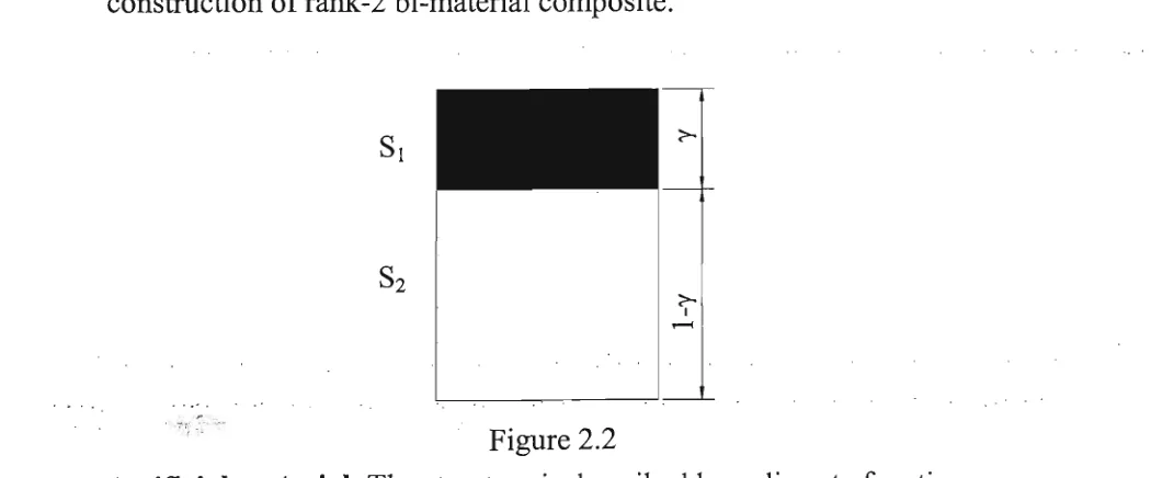
R a n k e d layered material cells: Each cell of this type of microstructure is

constructed from layers of different material. Figure 2.2 illustrates the construction of rank-2 bi-material composite.

Figure 2.2

Artificial material: T h e structure is described by a discrete function as

Z(x)

(34)

where Q is the design domain.

The solution of the optimization problem involves the determination of

effective (homogenized) material properties of micro structures. There are two methods for finding the effective material properties of microstructures and they can be expressed as follows:

• Numerical approach: In this approach, finite element models for the microstructure are constructed and appropriate boundary conditions for the periodicity are applied. A series of finite element analyses are carried out for voids of different sizes. In order to obtain a continuous variation of the homogenized material properties with respect to the void sizes, an

interpolation process can be applied to the "discrete" results from the finite element analyses.

• Analytical approach: In this approach, explicit expressions for the effective elastic tensor can be obtained by establishing the optimal upper and lower bounds for the complementary elastic energy density of the

perforated material. These microstructures are known as "external"

(35)

Once the effective material properties of the microstructure are determined,

they will be used as input data for the normal finite element analysis of the

structure, which is to be optimized. The unknowns in this problem are an array

of densities (and orientations of the holes for some types of microstructures). In

the optimization module, considering the geometrical parameters of the

presumed material model in finite elements as design variables, the total

potential energy is adopted as the objective function. The volume of material is

considered as the global constraint that has to be active. Using the optimality

criteria method, an updating scheme is constructed.

2.3.5 EVOLUTIONARY STRUCTURAL OPTIMIZATION METHOD

(ESO METHOD)

(36)

behaviour due to element removal. Xie and Steven (1994b, 1996, and 1997) also used the ESO method to optimize structural frequencies and buckling loads. The frequency of a structure can be shifted in a desired direction by removing material from the design domain based on a sensitivity analysis. A typical ESO method procedure is given as follows:

• Step 1; Model the structure using finite elements. Assign material properties, applied loads and boundary conditions. The design and non-design domains are defined.

• Step 2: Carry out finite element analysis (FEA) for the structure to obtain the structural behaviour i.e. element stresses, mean compliance or

constrained displacements.

• Step 3: Compute the sensitivity number for each element. The sensitivity number is a number representing the change in structural behaviour due to element removal.

• Step 4: Remove elements that have the lowest sensitivity numbers.

• Step 5: Repeat Steps 2 to 4 until one of the constraints is violated.

(37)

single iteration in order to maintain the smooth change between two successive iterations. Although the ESO method proves to be a reliable and efficient tool, there are drawbacks in the procedure that need to be improved. The

deficiencies of the ESO method are listed below:

• Because of the assumption that the global stiffness matrix of the structure does not change significantly in a single iteration, only a small number of elements can be removed at each iteration.

• There is no rationale to determine the removal ratio for a specific problem. The removal ratio is the number of elements removed in each iteration

over the number of all elements in the initial design or the number of all elements in the current design. So far, this number has been assigned based on the experience of the ESO users.

• There is no method for deciding which topology generated in the

evolutionary process is the optimum. Previous studies decide the optimum topology when the prescribed number of iterations is reached or the specified amount of material that is allowed to be removed from the design is reached. These assumptions are quite arbitrary.

(38)

the fact that different types of elements in the model cause it to become highly non-linear.

Yang (1999) developed the so-called bi-directional evolutionary structural optimization method (BESO method). In the BESO method, elements can be removed from as well as added to the model to obtain the optimum. Although BESO method starts with the simplest initial design connecting the load and supports, the maximum design domain in which the structure is allowed to

occupy must also be defined. In other words, these elements are still stored in

the data file but they do not physically exist as part of the structure in the initial design. By adding and removing elements simultaneously in the optimization

procedure, the BESO method has many advantages according to Yang (1999).

• As the BESO method starts from the simplest initial design, the degree of dependency of the optimal result on the initial design may be less than the ESO method which starts from an over-sized full design.

• By starting from the simplest initial design, the computational time and cost needed to carry out the finite element analysis for the model in the BESO method is dramatically less than that in the ESO method, which

(39)

enough, it m a y lead to computational times in the B E S O procedure greater than times for the ESO method.

• In the BESO method, elements that are removed prematurely can be recovered. This makes the method more reliable than ESO method. The BESO method also has some disadvantages:

• In some cases, the designer may only need a better design rather than a theoretically optimal solution. On one hand, this may be satisfied with the ESO method that starts from a feasible design. On the other hand, the

BESO method starts from an infeasible design and all the intermediate solutions lie in an infeasible region.

• Compared with the ESO method, the BESO procedure requires more parameters that have to be specified by the users.

Compared with other methods, the ESO method is likely to be the most

efficient method with acceptable reliability. Liang (1999a, 1999b, and 2000) proposes a method called the performance-based optimization method for

structural topology and shape design. It employs the ESO method in the

element elimination procedure and uses a scaling technique at the end of each iteration to monitor and determine the optimal topology (Liang, 2000). This method has proved reliable for 2D continuum structures in which the global

(40)

for structures with a combination of discrete and continuum elements, Liang's

performance index is no longer valid.

2.4 COMMENTS ON CURRENT RESEARCHES AND

APPLICATIONS

Despite significant effort directed towards the study of structural optimization

in the past, most studies have been restricted to the area of sizing or

geometrical optimization problems. Much less effort has been spent on

topological optimization that could result in most significant material savings.

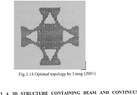
Furthermore, as stated by Liang (2001), structural optimization techniques

could become more attractive to civil engineers if they are developed not only

for saving materials but also for simplifying the designer's task by automating

the major design process.

For building structures, the appropriate method for structural optimization

needs to have the following features:

• Capable of dealing with large-scale structures. For example, buildings

with more than 50 storeys and multiple bays. The data entry and output

handling tasks need to be automated.

(41)

• Capable of solving structures with combination of discrete and continuum

elements. For example, shear wall-frame building where beams and

columns are modelled by beam elements and shear walls are considered as plate elements.

• Capable of dealing with both 2D and 3D models.

• Capable of dealing with multiple load cases.

• Capable of dealing with multiple support environments.

• Capable of dealing with multiple material environments.

Most of the commercial FEA packages available satisfy most of the items

shown above. In this thesis, the ESO method will be extended for dealing with structures containing both beam and continuum elements. The method

(42)

CHAPTER 3: THE EXTENDED ESO METHOD FOR OVERALL STIFFNESS CONSTRAINT

CHAPTER 3: THE EXTENDED ESO METHOD FOR

O V E R A L L S T I F F N E S S C O N S T R A I N T S

3.1 INTRODUCTION

A review on the development and applications of structural optimization methods

has been presented in Chapter 2. In this chapter, the extended E S O method for

continuum topology optimization subject to overall stiffness constraints will be

developed. Firstly, the topological structural optimization problem is stated for

seeking the optimal topology of a structure subject to overall stiffness constraints.

T h e optimal topology will be the one which has the same weight as the initial

structure, but has the m a x i m u m stiffness compared with all other topologies that

are generated during the optimization process. Secondly, sensitivity analysis will

-be carried out to derive the element removal criteria. Thirdly, termination criteria

and techniques to overcome sharp change in the m e a n compliance value of the

structure will also be discussed in order to complement the method. Finally, three

examples representing different types of finite element models will be presented to

demonstrate the validity and effectiveness of the extended E S O method.

3.2 OPTIMIZATION PROBLEM STATEMENT

u

**In the ESO method*'for overall stiffness constraints, the task of the designer is to ra^**

(43)

expressed as: C-C* <0 where C and C*are the mean compliance value and its

prescribed limit for the structure, respectively. Flowever, in practice, the mean compliance limit of the structure is usually unknown in advance.

By removing inefficient elements at each iteration, there will be a number of topologies generated during the optimization process. In order to determine the topology which has the maximum stiffness, it is natural to scale the topologies so that they all have the same weight and then their stiffnesses can be compared with each other. The topological structural optimization problem for overall stiffness constraint can be stated as:

Starting from an initial structure, the topological structural optimization problem

for overall stiffness constraint is to find the structural topology which has the same

weight as that of the initial structure and has the minimum mean compliance

value.

(44)

3.3 ELEMENT REMOVAL CRITERIA BASED ON STRAIN ENERGY

DENSITY

Before developing the strain energy density formulation, it is useful to present some definitions and theoretical concepts used in the ESO method.

The variable X;: As defined by Yang (1999), in the ESO method for topological

design of structure, the design variable is a non-dimensional quantity. For beam

A.

elements, it is defined as x, = — - where zL and A, are the sectional area of the

A

bar before and after being removed respectively. This means that _t. only receives value 0 (after elimination) or A0i (before elimination). Therefore, xt only receives value 0 or 1. Similarly, for continuum elements, xt is defined as x{ = — where tQi

hi

and t, are the thicknesses of the continuum elements before and after being removed, respectively.

In finite element analysis (FEA), the static behaviour of a structure is represented by the following equilibrium equation:

Ku = P (3-1)

where K is the global stiffness matrix, wis the displacement vector and P is the

external load vector.

(45)

C = -Pru (3.2) is c o m m o n l y used as the inverse measure of the overall stiffness of the structure. C is also known as the mean compliance of the structure.

Differentiating equation (3.1) with respect to the ith design variable, the result is:

8K „ du . -u + K— = 0

dx, 3X;

(3.3)

du

dx,

AdK

-K~

v

—u

8X:

(3-4)

F r o m equations (3.2) and (3.4) w e have:

dx; 2

f -K \ _,dK dx, i y (3.5)

Because the global stiffness matrix K is a symmetrical matrix, thus

8C 1 TdK

= — u u

dXi 2 dxt

Using the first term of a Taylor series expansion, w e obtain

(3.6)

dc

AC = C'-C = S^Ax,=-VS^Ax,

1=1 dx

8K

M 9x;

u (3.7)

where C i s the m e a n compliance of the structure after element removal and m is the total number of elements removed in the iteration.

Because the ESO process is a. 0-1 decision scheme, elements are gradually removed from the structure. Thus

1 T

AC = ~-uT

2

dK

IfMO-1)

1

T

2

f

2>, «^£«/

r

*/"/=£

c

* (3.8)

(46)

where

ut is the displacement vector of the i th

element.

C,. = —ufKiUi is the strain energy of the ith element.

In the ESO method the continuum design domain is usually divided into a finite element mesh of identical elements, and all the elements have the same volume. Therefore the element strain energy above can be successfully used as a driving force for the optimization process. However, for a model with finite elements of different shapes or sizes, the strain energy density of the ith element is defined as 1 T

—u, K,u,

r\ I It

^ = 2 (3.9)

w,

where wt is the weigh of the i th

element.

In the ESO process for continuum topology design with stiffness constraint, the elements with the lowest strain energy densities will be automatically removed at each iteration. To ensure a smooth change between two consecutive iterations, only a small number of elements are removed from the model.

3.4 STRUCTURE UNDER MULTIPLE LOAD CASES

In the case of multiple load cases, the procedure of deriving the strain energy

(47)

T

«-=^ ~ ~ (3.10)

_u

w.

where u

i}

is the displacement vector of the i

th

element due to they'* load case.

The element strain energy density under multiple load cases is defined as the sum

of the strain energy density due to each load case.

j

«,=2X (3.H)

/=i

where J is the number of load cases.

3.5 UNIFORMLY CHANGING THE THICKNESS OF CONTINUUM

ELEMENTS

Uniformly changing the thickness of continuum elements is often referred to as

scaling the structure. Scaling technique has been proposed by many researchers

(Kirsch, 1993; Morris, 1982 and Liang, 2000). As stated by Kirsch, the great

advantage of the scaling technique is that it can convert an infeasible design into a

feasible one. For example, in topological continuum optimization, by uniformly

changing the thickness of the continuum elements, the topology of the structure

unchanged, the designer can change the stiffness or displacements of a model from

an unaccepted value to an acceptable one.

(48)

(

P = ~ (3.12)

X

where x and x' are the vector of design variable before and after scaling,

respectively.

If the global stiffness matrix of the model is a linear function of the z

th

order of the

design variable, i.e.

K = C (3.13)*

where C is a constant, then the global stiffness matrix of the model after scaling

:.K =Cx'

z

= C{cpx)

z

=cp

z

Cx

2

= cp

z

K (3.14)

From equations (3.1) and (3.14) and assuming the scaling does not affect the

applied load, we have

K~x 1

u

>=K'-l

P = P = — u (3.15)

cp

z

(p

z

The mean compliance of the structure after scaling becomes

v

l

..iTzr.. if U }(„,„{

U

1_ 1

l

..T~ 1

C=-u" K'u

v) H

u

T

Ku = — C (3.17)

<p

z

2 (p

z l i\(p ) \cp )

For truss elements: The element stiffness matrix is a linear function of the

width of cross-sectional area. Thus z=l

C=-C (3.18)

For plane stress finite elements: The element stiffness matrix is a linear

(49)

design variable instead of the cross-sectional area of the truss member.

• For plate bending elements: The element stiffness matrix is a linear function of the 3rd order of the thickness of the plate. Thus z=3

C=\c (3.19)

9

• For general plate and shell elements: They have both in-plane and flexural

action. For small deflections, these two actions are independent. Therefore, it is assumed that flexural deflections and rotations of the element are only related to the forces normal to the plane and the in-plane displacements are only related to the in-plane forces. The element stiffness matrix consists of two parts, namely in-plane behaviour term and bending behaviour term.

K = KP+Kb (3.19)

where p denotes in-plane behaviour and b denotes bending normal to the plane. From equations (3.14) and (3.19)

K*=(pKP+(p'Kb (3.20)

For this type of elements, the problem becomes non-linear and the scaling

(50)

Liang (2000) proposed a method to monitor and select the optimal topology by calculating the performance index of each design that is generated in the ESO process. He defined a performance index

c w

PI = ^!Z!L (3.2i)

c

iwi

where PI: performance index of the current structure.

C0, Q: mean compliance the initial structure (ground structure) and

the current structure, respectively.

W0, W{. the weigh of the initial structure and the current structure,

respectively.

According to Liang (2000), the optimal topology is the one which has the highest PI value. However, this method is based on the assumption that the global stiffness matrix of the structure is a linear function of the zth order of the design variables. As shown in equation (3.20), this method is invalid when applied to structures

containing general plate and shell elements, as of 3D structures or structures containing different types of finite elements.

In order to solve the above problem, this thesis proposes a new procedure for comparing the structural performance of general 2D and 3D topologies. In each

iteration,.after removing inefficient elements, the thickness of the plate elements will be uniformly changed ("scaled") to make the weight of the current structure

(51)

thickness of the current structure and of the initial structure can be expressed as

pAt0n0=pAtknk (3.22)

•'•hno=tknk (3-23)

where p : the weight density of the material used.

A: the area of one continuum element, which is the same for all

elements.

t0,tk: the thickness of the continuum elements of the initial structure

and the current structure at kth iteration, respectively.

n0,nk: The total number of continuum elements of the initial

structure and the current structure at k*h iteration, respectively.

From equation (3.23), it can be shown that tk can be calculated from the element thickness of the previous iteration, i.e.

h ~ h-\

n k-\

n_k

(3-24)

After changing the thickness of the elements, a n e w finite element analysis will be

carried out to compute the mean compliance of the current design. This value will be saved into a database. At the end of the optimization process, based on the mean compliance history, the optimal topology will be picked from among many

(52)

3.6 TERMINATION CONDITIONS

In the ESO method, several criteria for stopping the optimization process have been proposed before. Xie and Steven (1994), in the original ESO method,

proposes to stop the process when the volume of the current structure reaches a prescribed value, says 50% of the initial structure. This criterion is arbitrary because it does not guarantee that the optimal topology is included in the

optimization process. The performance-based topological optimization method proposed by Liang (2000) states that the optimization process is terminated when the performance index of the current structure is greater than that of the initial structure. This termination condition is rigorous as it means the performance of the current structure, at that iteration, is even worse than the performance of the initial structure and hence the optimization process should be terminated.

However, Liang's termination condition may not be applied to general 3D structures or structures with a combination of beam and plate elements.

In this thesis, the optimization process is terminated when there is no more

decrease in the mean compliance of the equally weighted topologies. In the

(53)

3.7 HANDLING SHARP CHANGE IN THE MEAN COMPLIANCE

VALUES

The basic assumption of the ESO method for continuum topology optimization is

that the global stiffness matrix of the structure is not changed significantly within an iteration. It means that a smooth change in the topology of the structure must be kept between consecutive iterations. If this requirement is violated, the values of the mean compliance will change sharply and the structure may become a

mechanism (thus unstable). To keep the changes of the mean compliance between

consecutive iterations to be small, it is necessary to restrict the number of elements removed in each iteration by specifying a removal ratio. The removal ratio is

defined as the ratio of the number of elements to be removed to the total number of

elements of the initial or current structure. If the removal ratio is based on the

initial structure, the number of removed elements in each iteration is kept constant during the whole optimization process. If the removal ratio is based on the current structure, the number of removed elements in each iteration is gradually decreased during the optimization process and hence the computational cost is increased. However, it is worth using a removal ratio based on the current structure as the accuracy of solution is improved.

(54)

each iteration is small. Consider two consecutive iterations i and i+1 where there is a sharp change in the mean compliance values between them, the elements removed in the ith iteration must have played an important role in foiming the

global stiffness matrix of the structure. Therefore, to correct this problem, we can go back to the ith iteration and force the optimization process to remove other

elements instead. In the computer code, the elements removed in the /' iteration, which have caused the sharp change, will be recovered temporarily and fixed and the program will look for other elements to remove. It is noted that, after

temporarily recovering and fixing the elements, because the weight of the current structure has been increased, the thickness of the continuum elements needs to be uniformly reduced to keep the weight the same as the initial structure.

The technique of handling sharp changes in the mean compliance values can be illustrated in Figure 3.1.

Recover the elements remove in iteration n-1 and temporarily fix Sharp change occurs these_elements

Iteration n-1 Iteration n Iteration n+1

Decrease the current thickness t„ to the thickness of iteration n-1 (t„.,)

Fig.3.1 Technique of handling sharp change in the m e a n compliance values

(55)

temporarily fixed elements be released only if the optimization process finds other elements to remove without causing the sharp change in the mean compliance

value. The temporarily fixed elements can only be released when one of the conditions listed below is met.

• The number of temporarily fixed elements reaches a fixed ratio Is

defined by the ratio of the number of the temporarily fixed elements to the number of total elements of the current structure.

• After a successful iteration involving element removal. A successful iteration involving element removal is defined as an iteration in which elements are removed without causing sharp change in the mean compliance

value. This means that the optimization process is successful in finding a new way of removing elements for evolution. The temporarily fixed elements now can be released and allowed to participate in the future evolution.

(56)

Temporarily fix elements removed at the previous iteration

N u m b e r of the fixed elements greater than fixed ratio

Release all the temporarily fixed elements Iteration n- _{Iteration n}

Iteration n+1

Fig.3.2 Releasing temporarily fixed elements w h e n the number of temporarily fixed

elements is greater than fixed ratio

Sharp change does not occurs at this iteration

Successfully remove low strain energy density elements

Iteration n-1 Iteration n

Release all the temporarily fixed elements

• Iteration n+1

Fig.3.3 Releasing temporarily fixed elements after an iteration involving element removal

3.8 DESIGN PROCEDURE

The design procedure for topological structural optimization for overall stiffness

constraint is outlined as follows

Step 1; The structure is modelled using finite elements. The beam elements are

considered as a non-design domain. Their sizes and shapes are not changed

during the optimization process. Only continuum elements are considered as the

design domain and allowed to be removed during the optimization process. This

model is called an initial structure.

Step 2: Carry out the finite element analysis to compute the mean compliance of

(57)

equation (3.10).

Step 4: If there is a sharp change in the mean compliance value, temporarily fix

those elements removed at the previous iteration. Return the thickness of

continuum elements to the thickness value of the previous iteration. Repeat from Step 2.

Step 5: If the number of temporarily fixed elements is greater than or equal to the

fixed ratio, release all the temporarily fixed elements. Repeat from Step 2.

Step 6: Remove elements which have the lowest strain energy density from the

structure. The number of removed elements is equal to the removal ratio (RR) multiplied by the number of elements of the current structure.

Step 7: If there is no sharp change in the mean compliance value at the previous

iteration, release all the temporarily fixed elements.

Step 8: Uniformly increase the thickness of continuum elements in the design

domain by using equation (3.24).

Step 9: Save the current structure.

Step 10: Repeat from Step 2 to Step 9 until the termination condition in Section

(58)

Step 11: Plot the m e a n compliance history and select the optimal topology.

(59)

( Start)

jr.

Discretize the initial structure using finite elements.

Carry out finite element analysis for the current structure. ^

I

Calculate the strain energy density of each continuum element in the design domain by using equation (3.10).

Y

N

Release all the temporarily fixed elements.

Save the current structure

Return the thickness of continuum elements to the thickness value of the previous iteration.

Temporarily fix elements that have been removed at the previous iteration.

R e m o v e R R | ( % ) elements with the lowest strain energy density.

Release all the temporarily fixed elements.

Uniformly increase the thickness of continuum elements by equation (3.24)

N

Plot the m e a n compliance value history and select the optimal topology. • End

(60)

3.9 EXAMPLES

In this section, three examples are provided to demonstrate the effectiveness of the proposed method. Firstly, topological optimization for overall stiffness for a plane stress problem is solved. Secondly, a structure with plate elements (bending only) is considered. Finally, the topological optimization problem of a 3D structure containing both continuum and beam elements is solved.

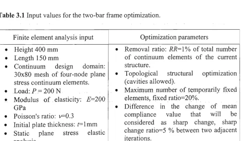
3.9.1 A PLANE STRESS STRUCTURE (TWO-BAR FRAME)

The efficiency and reliability of the proposed method is first examined by solving the well-known two-bar frame problem shown in Figure 3.5. The structural

optimization problem is to determine the optimal geometry of the frame under a point load P subject to overall stiffness constraint. This problem has been analytically solved by Rozvany (1976). If the frame structure is assumed to be a truss for the minimum-weight design, its optimal height H is obtained as H = 2L. Later, Suzuki and Kikuchi (1991) obtained the same result by using the

homogenization method.

Figure 3.6 shows the initial design for the optimization process. In order to achieve the optimal solution, it is necessary to have the initial design domain larger than the resultant two-bar frame structure. The continuum design domain is divided

(61)

Poisson's ratio is 0.3. The initial value of the thickness of continuum elements is lmm. The finite element analysis input and optimization parameters are listed in Table 3.1.

/

Design domain divided into 30x80 finite elements

400

150

200N

Fig.3.5 Optimal geometry of

the two-bar frame structure.

Fig.3.6 Initial design of the

optimization process.

Table 3.1 Input values for the two-bar frame optimization.

Finite element analysis input • Height 400 m m

• Length 150 m m

• Continuum design domain: 30x80 m e s h of four-node plane stress continuum elements. • Load: P = 200 N

• Modulus of elasticity: E=20Q G P a

• Poisson's ratio: v=0.3

• Initial plate thickness: £ = l m m • Static plane stress elastic

analysis.

Optimization parameters

• Removal ratio: RR=l% of total number of continuum elements of the current structure.

• Topological structural optimization (cavities allowed).

• M a x i m u m number of temporarily fixed elements, fixed ratio=20%.

(62)

The m e a n compliance history of the two-bar frame structural optimization subject

to overall stiffness constraint is given in Figure 3.7. It is seen from Figure 3.7 that the mean compliance of the structure gradually decreases during the process. In

other words, the overall stiffness of the structure is increasing during the

optimization process. The straight line AB indicates that the optimization program cannot remove any more elements without causing the structure to collapse.

Therefore, there is no improvement obtained during those iterations. The minimum mean compliance value was 0.167, which was obtained at iteration 93, and the corresponding topology is the optimal topology, as shown in Figure 3.8 (c). It is observed that the optimal topology also results in H=2L, which agrees well with the results of other researchers.

4.50E-01 -i ; — « 4.00E-01 -—

« 3.50E-01 - ^ v " 8 3.00E-01 ^

| 2.50E-01 ^ * > ^ ^

£ 2.00E-01 ^ ^ ^ ^ ^ A B 8 1.50E-01

| 1.00E-01 5 5.00E-02

0.00E+00 -I 1 ~< ' ' ' ' 0 20 40 60 80 100 120 140

Iterations

(63)

(a) Topology at (b) Topology at (c) Optimal topology iteration 30. iteration 50. at iteration 93.

Mc=0.316 Mc=0.239 Mc=0.167

Fig.3.8 Optimal topologies and m e a n compliance.

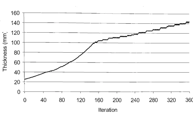
The thickness of the continuum design domain increases during the iterative

optimization process to ensure the topologies generated have the same weight as

that of the initial structure (see Figure 3.9). The zig-zag section AB indicates that

the optimization program is only fixing and releasing elements during those

(64)

0 20 40 60 80 100 120 140

Iterations

Fig.3.9 History of element thickness

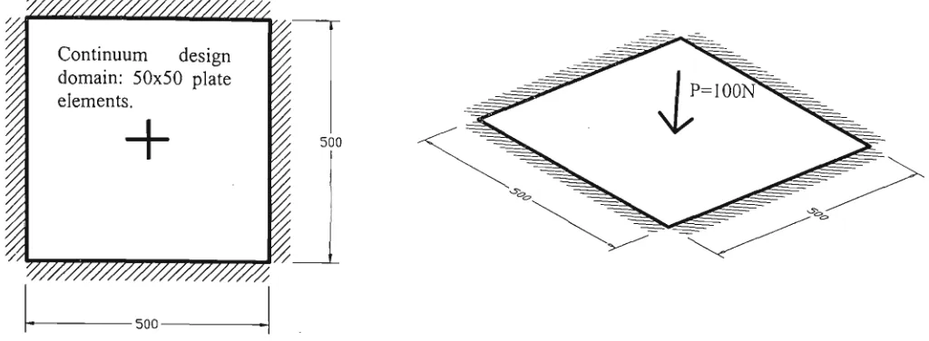
3.9.2 A PLATE IN BENDING

T h e extended E S O method is further examined b y solving a plate in bending

problem. A plate is fully fixed along its four edges and is loaded at the centre by a point load P=100N. Figure 3.10 shows the geometry of the plate under the