Article 1
A theoretical study and numerical simulation of a
2quasi-distributed sensor based on the low-finesse
3Fabry-Perot interferometer: Frequency-division
4multiplexing
5José Trinidad Guillen-Bonilla1,2, Alex Guillen Bonilla3, Verónica M. Rodríguez Betancourtt4, 6
Héctor Guillen Bonilla4, Antonio Casillas Zamora1 7
1 Computing and Electronic Departments, Centro Universitario de Ciencias Exactas e Ingenierías (CUCEI), 8
University of Guadalajara, Blvd. M. García Barragán 1421, Guadalajara, Jalisco 44410, México; e-mail:
9
[email protected]; [email protected];
10
2 Mathematic Department, Centro Universitario de Ciencias Exactas e Ingenierías (CUCEI), University of 11
Guadalajara, Blvd. M. García Barragán 1421, Guadalajara, Jalisco 44410, México; e-mail:
12
3 Departamento de Ciencias Computacionales, Centro Universitario de los Valles, Universidad de 13
Guadalajara, Ameca Km 45.5, C.P. 46600, Ameca, Jalisco, México. Ameca, Jalisco, México. e-mail: 14
15
4 Materials Science Graduate School, Centro Universitario de Ciencias Exactas e Ingenierías (CUCEI), 16
University of Guadalajara, Blvd. M. GarcíaBarragán 1421, Guadalajara, Jalisco 44410, México. E-Mails: 17
veró[email protected]; [email protected]
18 19
* Correspondence: [email protected] Tel.: 01 (33) 13 78 59 00 ext. 27655 20
21 22
Abstract: The application of the sensors optical fiber in the areas of scientific instrumentation and 23
industrial instrumentation is very attractive due to its numerous advantages. In the industry of civil 24
engineering for example, quasi-distributed sensors made with optical fiber are used for reliable 25
strain and temperature measurements. Here, a quasi-distributed sensor in the frequency domain is 26
discussed. The sensor consists of a series of low-finesse Fabry-Perot interferometers where each 27
Fabry-Perot interferometer acts as a local sensor. Fabry-Perot interferometers are formed by pairs of 28
identical low reflective Bragg gratings imprinted in a single mode fiber. All interferometer sensors 29
have different cavity length, provoking the frequency-domain multiplexing. The optical signal 30
represents the superposition of all interference patterns which can be decomposed using the Fourier 31
transform. The frequency spectrum is analyzed and sensor´s properties were defined. Following, a 32
quasi-distributed sensor was numerically simulated. Our sensor simulation considers sensor 33
properties, signal processing, noise system and instrumentation. The numerical results show the 34
behavior of resolution vs. signal-to-noise ratio. From our results, the Fabry-Perot sensor has high 35
resolution and low resolutions. Both resolutions are conceivable because the FDPA algorithm 36
elaborates two evaluations of Bragg wavelength shift. 37
Keywords: Quasi-distributed sensor; Low-finesse Fabry-Perot interferometer; Sensor simulation; 38
Frequency-domain multiplexing and resolution vs. signal-to-noise ratio. 39
40
1. Introduction 41
Bragg grating has a very particular peak in its reflection spectrum, that one is centered at the 42
Bragg wavelength = 2 Λ [1]: Λ is the grating pitch and is the effective fiber refraction index. 43
The operational principle of fiber Brag grating sensor is based on the spectral shift of the central Bragg 44
change on the grating. The monitoring system needs to detect the wavelength shift with very high 46
resolution, permitting its correct evaluation. This shift is evaluated from optical measurements, for 47
example: a dual-OFC FBG interrogation system [2], tunable Fabry-Perot filter with a piezoelectric 48
actuator [3] and direct spectroscopic detection [4]. 49
Bragg gratings play an important role in the fiber-optic sensor technology. Such sensors are very 50
attractive for quasi-distributed sensing employing only one optical fiber with many gratings printed 51
along a fiber length. The conventional Bragg grating sensors use a broadband light source and a direct 52
spectrometric detection technique. Its principal problem concerns to the detection of relatively small 53
shifts in resonant wavelength of gratings array exposed to the strain or slow temperature changes. 54
An additional application of Bragg gratings in sensor technology is to build interferometers within 55
the single path fiber. In this case, Bragg gratings act as selective mirrors. The positions of gratings 56
along the fiber length define the optical path difference. Frequency-division multiplexing, 57
wavelength-division multiplexing and time-division multiplexing can be implemented [5-12]. 58
The twin-grating fiber optic sensor was used for the temperature measurement. The optical 59
sensor acts as a low-finesse Fabry-Perot interferometer and it consists of two identical Bragg gratings 60
separated by a short distance. The Fourier Domain Phase Analysis (FDPA) algorithm was used for 61
its signal demodulation. The FDPA algorithm evaluates the Bragg wavelength shift at the frequency 62
domain. The algorithm is based on the evaluation of the phase of the interference pattern produced 63
by light reflected from both gratings and on the determination of the Bragg wavelength shift. The 64
wavelength shift sensitivity was measured to 0.00985nm/oC [13]. This fiber sensor was also used for
65
the measurement of static strain. Resolution of 0.2 µm/m was reported [14]. 66
In reference [15], a quasi-distributed sensor was experimentally proposed. Twin-grating sensors 67
were applied as local sensors. Frequency-division multiplexing was implemented. Following, in 68
reference [16] this quasi-distributed sensor was described. The authors gave the next description: 69
Frequency-division multiplexing was applied. A tunable external cavity diode laser was used for the 70
sensor interrogation. The sensing systems consisted of a serial array of 14 twin grating sensors. All 71
Bragg gratings had the same length of 0.5 mm and reflectivity of 0.8%. The Bragg wavelength of all 72
gratings was 1550.6nm. The cavities were into the interval of 2 mm to 34 mm. The optical spectrum 73
was acquired. Their frequency components were separated applying the fast Fourier transform (FFT) 74
algorithm. There were 14 channels. Each channel was generated from each Fabry-Perot sensor. 75
Another quasi-distributed fiber optic sensors can be found in references [17-22]. 76
Under our knowledge, the quasi-distributed sensor described in Ref. [16] does not have an 77
analytic analysis. Therefore, local sensor limitations are not known. Here, a theoretical analysis and 78
numerical simulation is elaborated for the quasi-distributed sensor described in reference [16]. A 79
broadband light source, direct spectrometric detection technique and frequency-domain 80
multiplexing are considered in our study. Knowing its operation principle, the optical spectrum was 81
represented mathematically. We analyzed the optical signal and then the quasi-distributed sensor´s 82
properties were defined, for example: minimum and maximum cavities, number of samples, spatial 83
resolution and multiplexing capability of a twin-grating fiber sensor. All parameters are expressed in 84
terms of physical parameters and instrumentation characteristics. Following, the quasi-distributed 85
sensor was numerically simulated (in operation) and we obtain the graph of Demodulation errors vs. 86
signal-to-noise ratio. From our numerical results, the cavity length augments the resolution, all Fabry-87
Perot sensors have two resolutions: a high resolution and low resolution. The cavity length, low 88
resolution and noise system define the transition between both resolutions. In general, our theoretical 89
analysis and numerical simulation permit its optimal implementation and its design. 90
2. Optical signal 91
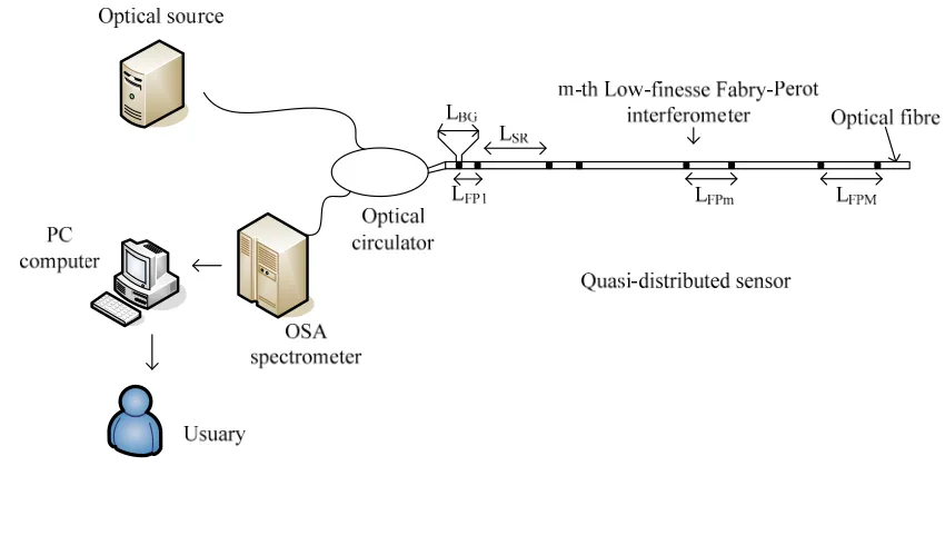
Fig. 1 shows our optical sensing system schematically. The optical system consists of a 92
broadband source, an optical circular 50/50, an optical analyzer spectrometer (OSA spectrometer), a 93
personal computer and a quasi-distributed sensor. The quasi-distributed sensor can be implemented 94
by using a serial array of low-finesse Fabry-Perot interferometers [15,16]. The local sensors are formed 95
interferometer has a unique optical path length, obtaining the frequency-division multiplexing 97
(FDM). The Bragg gratings have approximately the same length and typical reflectivity of 0.1%. Thus, 98
wavelength-division multiplexing was eliminated for our optical sensor. 99
Figure 1. Sensing system 100
2.1. ( ) and ( ) spectrums 101
When the quasi-distributed sensor does not have external perturbations, the optical signal ( ) 102
will be the superposition of all interference patterns, 103
( ) = ( ) = ( ) + ( ) + ( ) + ⋯ + ( ) (1)
( ) is the optical signal detected by the OSA spectrometer and ( ), ( ), ( ) … ( ) are
104
interference patterns generated by all interferometer sensors. Considering the physical parameters, 105
the optical signal can be re-written as [13] 106
( ) = 2 2 ( − ) 1 + 4 ( − ) (2)
where is the wavelength, are amplitude factors, is the amplitude of the effective refractive 107
index modulation of the gratings, is the length of gratings, is Bragg wavelength, is the
108
effective index of the core, is the ℎ cavity length and is the number of low-finesse Fabry-109
Perot interferometers (local sensors). Analyzing the optical signal (2), all interference patterns have a 110
similar enveloped function, the enveloped is the reflection spectrum of the gratings, the width Δ 111
is defined as the spectral distance between its +1 and -1 zeros, 112
Δ = (3)
Each interference pattern has its own frequency component. There are M modulate functions where 113
the frequency component will be
114
=2 (4)
( ) = ℱ ( ) = ( ) (5)
( ) is the frequency spectrum, ℱ is the Fourier operator and is the frequency. Substituting 116
Equs. (2), (3) and (4) into Equ. (5), the frequency spectrum is 117
( ) = 2 −
Δ 1 + 2 ( − ) (6)
Invoking the convolution properties and Fourier operator, we have 118
( ) = ℱ −
Δ ⊗ ℱ 2 1 + 2 ( − ) (7)
the symbol ⊗ indicates the convolution. Using the identities: ( ) = 1 + (2 ) , ( ) =
119
, ∑ = ∑ and solving, the frequency spectrum ( ) is
120
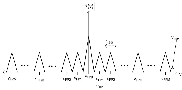
( ) = ( ) = − (8)
( ) spectrum is a set of triangle functions where are amplitude factors, is the bandwidth 121
=4 (9)
and are the center position of each triangle function. Here, all frequency components were
122
separated as Fig 2 illustrates 123
124 125
Figure 2. ( ) frequency spectrum 126
2.2. ( , ) and ( , ) spectrums 127
When the quasi-distributed sensor has external perturbations, the measured (temperature or 128
string) affects the gating period Λ, the refraction index , the length of gratings and cavity 129
length [13]. In turn, interference patterns has a small shift in response to a measured variation, 130
the optical signal detected by the OSA spectrometer is 131
( , ) = 133
2 2 ( − − ) 1 + 4 ( − − ) (10)
134
The optical spectrum ( , ) can be expressed as 135
( , ) = ( − ) = ( − ) + ( − ) + ⋯ + ( − ) (11)
where ( , ) is the optical signal due to external perturbations and is Bragg wavelength
136
shift due to measured change. Now, we estimate their frequency components through 137
( , ) = ℱ ( , ) = ( − ) (12)
Invoking the shift property and solving, the Fourier transform is 138
( , ) = ( ) (13)
Observing the Equ. (13), the frequency spectrum ( , ) is the multiplication between ( ) (Ecq. 139
8) and a set of phases. Those phases contain the information about the perturbations. 140
3. Cavity length 141
For all quasi-distributed sensors based on interferometers (optical fibre), the cavity length is a 142
very important parameter since it defines the sensor characteristics. Their limits depend of 143
instrumentation, local sensor characteristics and signal demodulation. Following, we determine 144
minimum and maximum cavities where the low-finesse Fabry-Perot interferometer can be applied. 145
3.1. Minimum cavity length 146
The Fourier Domain Phase Analysis (FDPA) algorithm was developed for the twin-grating fiber 147
optic sensor [13]. This algorithm does not accept additional information and does not accept the loss 148
information, therefore, good signal detection and good frequency component identification are 149
necessary. From Fig. 2, first frequency components can be defined by 150
= (14)
The condition (14) eliminates the overlapping between components, and . Using the Equs.
151
(4) and (9), we have 152
2
=4 (15)
As ≈ , the minimum cavity length will be
153
= 2 (16)
It´s not possible smaller cavities because the FDPA algorithm can not demodulate the optical signal. 154
3.2. Maximum cavity length 155
The optical sensing system applies the direct spectroscopic detection [4]. This technique uses an 156
optical spectrometer analyzer which defines the maximum cavity length . The OSA
157
spectrometer has a limit for the optical signal detection. The limit is the Full-With Half-Maximum 158
(FWHM). Considering the sampling theorem, the OSA spectrometer can detect the signal if and only 159
if next condition is true, 160
where Δλ is the minimum period detectable (FWHM) and Δλ is its spectrometer resolution. 161
Then, the maximum frequency component can be expressed as 162
= 1
Δλ (18)
From Fig. 2 and Equ. (4), last frequency component can be determined by
163
=2 (19)
Combining Equs. (17), (18) and (19), the maximum cavity length is 164
=
4 Δλ (20)
Equ. (20) indicates the maximum cavity length where OSA spectrometer can detect the optical signal. 165
It´s not possible bigger cavities because the instrumentation can not detect the optical signal. Using 166
Equs. (16) and (20), the cavity length can be into the interval of 167
2 ≤ ≤
4 Δλ (21)
4. Capacity of frequency-division multiplexing 168
In the quasi-distributed sensor, each low-finesse Fabry-Perot interferometer generates an 169
interference pattern and then each pattern produces a channel in the frequency domain. The 170
enveloped function produces the bandwidth and the modulate function provokes the frequency
171
components: − , and . The term contains information from all Fabry-Perot
172
interferometers while − and contain similar information from the mth Fabry-Perot
173
sensor. From Fig. 2, we have the next condition 174
= (22)
In other words, the capacity of frequency-division multiplexing is given by the relation
175
between last and first frequency components. Substituting the Equs. (14), (15) and (17) into (22), the 176
capacity can be re-written as 177
= (23)
Finally, substituting the Equs. (16) and (20) into Equ. (22), we have 178
=
8 Δλ (24)
This expression gives the limit for the multiplexing capacity within one wavelength channel. 179
4. Number of samples 180
When the optical spectrometer analyzer instrument acquires the optical signal, the reflection 181
spectrum is recorded as a series of digital samples. If a minimum and maximum wavelengths within 182
a working interval = − : is the maximum wavelength, is the minimum
183
wavelength and δ is the wavelength step. The signal samples ( ) are taken wavelengths =
184
+ where = 0,1,2, … , − 1, is the number of samples. The representation of such a
185
signal in Fourier domain is also discrete. Therefore, we obtain next condition from Fig. 2 186
≥ 2 = 2 +
2 (25)
where is the maximum frequency, is the sampling frequency and Nyquist theorem was
187
≥ 4 ( + 2 ) (26)
Since = , we have
189
δ ≤
4 ( + 2 ) (27)
Finally, the number of sample is 190
N = δ =
4 ( + 2 )
(28)
The number of samples depends of optical system parameters. 191
5. Digital demodulation 192
The demodulation is the complete signal processing algorithm developed for quasi-distributed 193
sensor based on the low-finesse Fabry-Perot interferometers. The complete processing algorithm 194
combines the Fourier Domain Phase Analysis (FDPA) algorithm and a bank of M filters. The FDPA 195
algorithm was described in Ref. [13] while the bank of filters is 196
F( ) = ⨂ ( − ) (29)
where the symbol ⨂ indicates the convolution operation, the rect function has next definition 197
rect( ) = 1 | | < 2 0 | | >
2
(30)
and is the Dirac delta. Invoking the Diract delta properties, the bank of M filters is 198
F( ) = − (31)
The bank filter of M filters is a series of rect function: is the central position and is its 199
bandwidth. 200
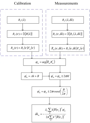
The digital demodulation consists of two phases: calibration and measurements. In the 201
calibration, there are four steps: 1) ( ) is acquired, 2) ( ) is computed, 3) ( ) is filtered 202
( ) = ( ) ( ) and 4) we calculate its complex conjugate ∗( ) where * indicates complex 203
conjugate. In the measurement, there are seven steps: 1) ( , ) is acquired, 2) ( , ) is
204
computed, 3) ( , ) is filtered ( , ) = ( , ) ( ), 4) the relative phase is calculated,
205
5) the ambiguity 2 is eliminated and then absolute phase is calculated and 6), 7) the Bragg 206
wavelength shift is computed, a digital adaptive filter is applied [23]. 207
Due to the presence of the noise in the original signal, the calculated phased will be fluctuating. 208
To minimize the noise influence and provide the best estimate, the absolute phase is multiplied with 209
a set of coefficients. Those coefficient act as an adaptive filter. The Fig. 3 illustrates the digital 210
demodulation schematically. 211
)
(
λ
T
R
( )
{
λ
}
ν
R
R
T(
)
=
ℑ
( ) ( )
ν
ν
ν
T mm
R
F
R
(
)
=
)
,
(
λ
δλ
T
R
(
)
{
λ
δλ
}
δλ
ν
,
)
,
(
TT
R
R
=
ℑ
(
ν
δλ
) ( )
ν
δλ
ν
T mm
R
F
R
~
(
,
)
=
,
(
~
*)
arg
m mm
=
R
R
ϕ
B
Ak
m
=
+
'
ϕ
ϕ
m'=
ϕ
m±
2
π
M
±
=
π
π
ϕ
ϕ
2
2
'
round
B
m m
( )
( )
−
=
k k
kj
m k w
m
R
k
R
k
2 2
' 2
~
2
~
ν
π
ϕ
ν
λ
δλ
Calibration
Meassurements
Figure 3. Digital demodulation represented schematically 213
6. Numerical simulation and discussion 214
6.1. Parameters and Results 215
To test and compare our theoretical analysis, we performed a numerical simulation of quasi-216
distributed sensor based on low-finesse Fabry-Perot interferometers. Three Fabry-Perot sensors were 217
simulated. Their physical parameters can be observed on Table 1. Discrete spectrums were simulated 218
using the physical parameters. Noise was simulated by adding, to those samples, pseudorandom 219
numbers with Gaussian distribution, the interval was from √ = 10 to √ = 10 . Typical of
220
Bragg gratings with rectangular profile at refractive index modulation was used. In most of our 221
numerical experiments, the number of samples was equal to 1024 (Fast Fourier transform algorithm 222
was considered). For each local sensor, the reference spectrum and 50 measurements were simulated. 223
The measurements were into the interval of, S10 to 0.2 nm, S20 to 0.4 nm and S30 to 0.7nm. 224
results: Demodulation errors vs SNR1/2. A Laptop Toshiba 45C was used, their properties were 512 of
226
RAM memory and velocity of 1.7 GHz. 227
Table 1. Quasi-distributed sensor parameters 228
Sensor number Sensor parameters Signal values
Low-finesse Fabry-Perot interferometer 1
(S1)
LFP1=4 [mm]
Δλ = 3.22[nm] (Equ. 3) = 4.95[Ciclos/nm] (Equ. 4) = 1.23[Ciclos/nm] (Equ. 9) LBG=0.5 [mm]
n=1.46
= 1532.5 [nm]
Low-finesse Fabry-Perot interferometer 2
(S2)
LFP2=8 [mm]
Δλ = 3.22[nm] (Equ. 3) = 9.91[Ciclos/nm] (Equ. 4) = 1.23[Ciclos/nm] (Equ. 9) LBG=0.5 [mm]
n=1.46
= 1532.5 [nm]
Low-finesse Fabry-Perot interferometer 3
(S3)
LFP3=16 [mm]
Δλ = 3.22[nm] (Equ. 3) = 19.82[Ciclos/nm] (Equ. 4) = 1.23[Ciclos/nm] (Equ. 9) LBG=0.5 [mm]
n=1.46
= 1532.5 [nm] 229
230
Figure 4. Optical signal ( ) 231
232 233 234 235
1532
1534
1536
1538
1540
0
0.1
0.2
0.3
0.4
0.5
0.6
0.7
0.8
0.9
1
λ [nm]
R
T(
λ
) [A
rb
itra
ry
U
n
its
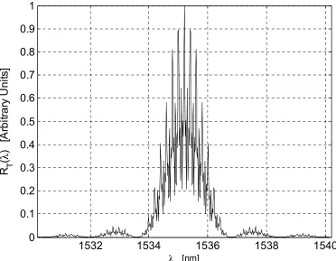
Figure 5. Optical signal ( ) 236
237 238
Figure 6. Numerical results 239
-20
-15
-10
-5
0
5
10
15
20
0
0.2
0.4
0.6
0.8
1
ν
[cycles/nm]
|R
T(
ν
)|
ν
FP1ν
FP2ν
FP3Filters F(
ν
)
100 101 102 103 104
10-7 10-6 10-5 10-4 10-3 10-2 10-1 100
Signal-to-noise ratio ,
SNR
1/2D
e
mo
d
u
la
tio
n
e
rro
rs
,
δλ
'
BGCavity Length: L'FP=4 mm L'FP=8 mm L'FP=16 mm Low resolution
240
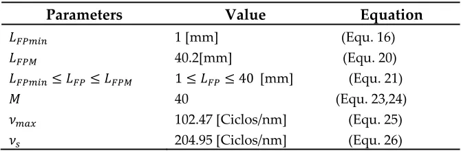
If the OSA spectrometer has Δ = 10 (typical value), the quasi-distributed sensor will have their 241
limits as Table 2 illustrates. 242
243
Table 2. Quasi-distribuido sensor limits (Δ = 10 ) 244
Parameters Value Equation
1 [mm] (Equ. 16) 40.2[mm] (Equ. 20)
≤ ≤ 1 ≤ ≤ 40 [mm] (Equ. 21)
40 (Equ. 23,24) 102.47 [Ciclos/nm] (Equ. 25) 204.95 [Ciclos/nm] (Equ. 26) 245
From Tables 1 and 2, the simulated quasi-distributed sensor satisfies the instrumentation and 246
signal requirements. Observing Table 1 and Figures 4, 5, numerical results are in concordance with 247
the theory. Thus, we confirm our theoretical analysis. Our numerical results can be observed at Fig. 248
6. 249
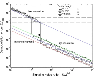
Fig. 6 shows the behavior Demodulation errors vs signal-to-noise rate SNR1/2. If the
250
demodulation error is denominated resolution then low-finesse Fabry-Perot has two resolutions: low 251
resolution and high resolution. Two resolutions are possible because the FDPA algorithm dose two 252
evaluations of Bragg wavelength shift [13,23]. All Fabry-Perot sensors have similar low resolution 253
however each local sensor has its own high resolution. The high resolution depends of cavity length. 254
If the cavity length is bigger then Fabry-Perot sensor will have better resolution. 255
6.2. Discussion 256
Based on our theoretical analysis and numerical simulation, the quasi-distributed sensor would 257
be built on the low-finesse Fabry-Perot interferometer. Our theoretical analysis optimizes its 258
implementation. Instrumentation, local sensor properties, noise (Gaussian distribution) and signal 259
processing were considered. The quasi-distributed sensor has good sensitivity and excellent 260
resolution. All Fabry-Perot sensors have two resolutions: low resolution and high resolution (See Fig. 261
6). Low resolution was obtained when Bragg wavelength shift was evaluated with enveloped 262
function. High resolution was obtained when Bragg wavelength shift was evaluated combining the 263
enveloped and modulate functions [13,23]. 264
When the noise is big, signal-to-noise ratio (SNR) is small. In this case, the FDPA algorithm can 265
not evaluate Bragg wavelength shift, causing the transition from high resolution until low resolution. 266
That one can be observed at Fig. 6. As the signal is (necessary) into the interval of – to and based 267
on the signal detection theory, the thresholding value is 268
3 <Δ
2 (32)
where is the low resolution (resolution by enveloped function) and Δ = is the period
269
of our frequency component. The threshold divides between low and high resolutions. Substituting 270
Equ. (4) into Equ. (32), we have 271
<
12 (33)
From Equ. (33), each low-finesse Fabry-Perot interferometer has its own thresholding value. This 272
one depends on the cavity length, Bragg wavelength and refraction index. For example: our Fabry-273
Perot sensors have next thresholding values, S10.033nm, S20.016nm and S30.008nm. The
274
In the quasi-distributed sensor, ghost interferometers are eliminated if the separation between 276
any two interferometers satisfy the expression > where is the spatial resolution. If
277
Fabry-Perot interferometers are formed by uniform unapodized gratings with equal length , the
278
bandwidth of each peak is given by Equ. (9). To be separated in the frequency domain, two peaks 279
should not overlap. This condition imposes the following constrains: the minimum distance between 280
centers of gratings for the shortest interferometers is 2 and the difference in the cavity lengths of 281
any two Fabry-Perot interferometers must exceed 2 .
282
Our future research work has the next directions: Wavelength-division multiplexing (WDM) can 283
be implemented based on the low-finesses Fabry-Perot interferometers. The theoretical resolution is 284
another direction. Technical applications are possible, for example: temperature, strain, humidity, 285
force measurement and oil detection. 286
7. Conclusions 287
The quasi-distributed optical fibre sensor based on the low-finesse Fabry-Perot interferometer, 288
was studied theoretically and simulated numerically. Theory and simulation are in concordance. Our 289
study considers quasi-distributed sensor properties, local sensor properties, signal processing, noise 290
source, frequency-division multiplexing and instrumentation. Our numerical results showed that all 291
Fabry-Perot sensors have two resolutions: low resolution and high resolution. Low resolution is 292
similar for all sensors however each Fabry-Perot sensor has its own high resolution. The thresholding 293
value (from high resolution to low resolution) was defined in terms of low resolution and physical 294
parameters. 295
The quasi-distributed sensor has potential industrial applications, for example: structure 296
monitoring, security system, humidity sensing and level sensing. 297
Acknowledgments: José Trinidad Guillen Bonilla thanks to CONACyT of Mexico by the scholarship. He also 298
expresses your acknowledgments to S. V. Miridonov for your counseling and comments. This work was began 299
at the CICESE and finished at the Guadalajara University. 300
Author Contributions: José Trinidad Guillen Bonilla performed the theoretical analysis and numerical 301
simulation. A. Guillen corroborated the numerical simulation. All authors wrote the paper. All authors read and 302
approved the final manuscript. 303
Conflicts of Interest: The authors declare no conflict of interest. 304
References 305
1. Kashyap R. Photosensitive Optical Fibers: Device and Applications. Optical Fiber Technology, 1994, 1, 17-306
34. doi: 10.1006/ofte.1994.1003 307
2. Posada-Roman J. E.; Garcia-Souto J. A.; Poiana D. A. and Acedo P. Fast Interrogation of Fiber Bragg Gratins 308
with Electro-Optical Dual Optical Frequency Combs. Sensors, 2016, 16,2007. doi:10.3390/s16122007
309
3. Di Sante R. Fibre Optic Sensors for Structural Healt Monitoring of Aircraft Composite Structures: Recent 310
Advances and Applications. Sensors, 2015, 15, 18666-18713; doi:10.3390/s150818666 311
4. Miridonov S. V.; Shlyagin M. G.; and Spirin V. V. Resolution limits and efficient signal processing for fiber 312
optic Bragg grating sensors with direct spectroscopic detection. Processing of Optical Measurements 313
Systems for Industrial Inspection III, Vol. 5144, Munich, Germany, 23-26 June 2003, Osten W.; Creath K.; 314
Kujawiska M. 315
5. Ben Zaken B. B.; Zanzury T. and Maka D. An 8-Channel Wavelength MMI Demodultiplexer in Slot 316
Waveguide Structures. Materials, 2016, 9,881; doi:10.3390/ma9110881 317
6. Huang J.; Zhou Z.; Zhang L.; Chen J.; Ji C. and Pham T. Strain _Modal Analysis of Small and Light Pipes 318
Using Distributed Fibre Bragg Grating Sensors. Sensors, 2016, 16, 1583; doi:10.3390/s16101583 319
7. Weng Y.; Ip E.; Pan Z. and Wang T. Advances Spatial-Division Multiplex Measurement Systems 320
Propositions-From Telecommunication to Sensing Applications: A Review. Sensors, 2016, 16, 1387; 321
doi:10.3390/s16091387 322
8. Ali T. A.; Shehata M. I. and Mohamed N. A. Design and performance investigation of a highly accurate 323
apodized fiber Bragg grating-based strain sensors in single and quasi-distributed systems. Applied Optics, 324
9. Cibula E. and Donlagic D. In-line short cavity Fabry-Perot strain sensor for quasi distributed measurements 326
utilizing standard OTDR. Optic Express, 2007, Vol. 15, No. 14, 8719-8730; 327
https://doi.org/10.1364/OE.15.008719 328
10. Kežmah M. and Ðonlagic. Multimode All-fiber quasi-distributed refractometer sensor array and cross-talk 329
mitigation. Applied Optics, 2007, Vol. 46, Issue 19, 4081-4091; htpps://doi.org/10.1364/AO.46.004081 330
11. Werzinger S.; Bergdolt S.; Engelbrecht R.; Torsten T. and Schmauss B. Quasi-Distributed Fiber Bragg Graint 331
Sensing Using Steppen Incoherent Optical Frequency Domain Reflectometry. Journal of Lightwave 332
Technology, 2016, Vol. 34, Issue 22, 5270-5277; 333
12. Yu Z.; Yang J.; Yuan Y.; Li C.; Liang S.; Hou L.; Peng F.; Wu B.; Zhang J.; Liu Z. and Yuan L. Quasi-334
distributed birefringence dispersion measurement for polarization maintain device with hihj accuracy 335
based on white light interferometry. Optic Express, 2016, Vol. 24, No. 2, 1587-1597; 336
DOI:10.1364/OE.24.001587 337
13. Miridonov S. V.; Shlyaing M. G. and Tentori D. Twin-grating fiber optic sensor demodulation. Optics 338
Communications, 2001, 191, 253-262. 339
14. Shlyagin M. G.; Swart P. L.; Miridonov S. V.; Chtcherbakov A. A.; Márquez Borbon I. and Spirin V. V. Static 340
strain measurement with sub-micro-strain resolution and large dynamic range using a twin-Bragg.grating 341
Fabry-Perot sensor. Optical Engineering, 2002, 41(8), 1809-1814; doi:10.1117/1.1489048 342
15. Shlyagin M. G.; Miridonov S. V. and Tentori D. Frequency multiplexing of in-fiber Bragg grating sensors 343
using tunable laser. Processing of Micro-optical for Measurement, Sensors, and Microsystems II and 344
Optical Fiber Sensor Technologies and Applications, Vol. 3099, Munich, Germany, September 24, 1997, 348; 345
doi:10.1117/12.281246 346
16. Shlyagin M. G.; Miridonov S. V.; Márquez-Borbón I.; Spirin V. V.; Swart P. L. and Chtcherbakov A. A. 347
Multiplexed twin Bragg grating interferometer sensor. Proceeding of Optical Fiber Sensors Conference 348
Technical Digest, OFS 2002, 10 May 2002, 191-194; doi:101109/OFS.2002.1000534 349
17. Trontz A.; Cheng B.; Zeng S.; Xiao H. and Dong J. Development of Metal-Ceramic Coaxial Cable Fabry-350
Perot Interferometer Sensors for High Temperature Monitoring. Sensors, 2015, 15, 24914-24925; 351
doi:10.3390/s151024914 352
18. Li X.; Sun Q.; Liu D.; Liang R.; Zhang J.; Wo J.; Shum P. P. and Liu D. Simultaneous wavelength and 353
frequency encoded microstructure based quasi-distributed temperature sensor. Optics Express, 2012, Vol. 354
20, No. 11, 12076-12084 355
19. Tao Y. J.; Ran Z. L. and Zhou C. X. Fiber-optic Fabry-Perot sensors based on a combination of spatial-356
frequency division multiplexing and wavelength division multiplexing formed by chirped fiber Bragg 357
grating pairs. Applied Optics, 2006, Vol. 45, Issue 23, 5815-5818; htpps:doi.org/AO.45.005815 358
20. Rao Y. J.; Henderson P. J.; Jackson D. A.; Zhang L. and Bennion I. Simultaneous strain, temperature and 359
vibration measuremen using a multiplexed in-fibre-Bragg-grating/fibre-Fabry-Perot sensor system. 360
Electronics Letter, 1997, Vol. 33, No. 24, 2063-2064; doi:10.1049/el:19971409 361
21. Martinez-Manuel R.; Shlyagin M. G.; Miridonov S. V. and Meyer J. Vibration Disturbance Localization 362
Using a Serial Array of identical Low-Finesse Fiber Fabry-Perot Interferometers. IEEE Sensors, 2012, Vol. 363
12, Issue 1, 124-127; doi:10.1109/JSEN.2011.2119479 364
22. Viet Nguyen L.; Vasiliev M. and Alameh K. Three-wave Fiber Fabry-Perot Interferometer for Simultaneous 365
Measurement of Temperature and Water Salinity of Seawater. IEEE Photonics Technology Letters, 2011, 366
Vol. 23, Issue 7, 450-452; doi: 10.1109/LTP.2011.2109057 367
23. Miridonov S. V.; Shlyaing M. G. and Tentori D. Digital demodulation of twin-grating fiber-optic sensor. 368
Proceeding of Conference on Fiber Optic and Laser Sensor and Application, Vol. 3541, Boston, 369
Massachsetts, USA, 1998, 33-40. 370
© 2017 by the authors; licensee Preprints, Basel, Switzerland. This article is an open 371
access article distributed under the terms and conditions of the Creative Commons by 372