Abnormality Detection in Digital Mammogram
S Narasimha Murthy #1, Arun Kumar M N #2, H.S. Sheshadri *3 #1
Research Scholar, PET Research Center, Mandya, Karnataka
#2
Associate Professor, FISAT, Ernakulam, Kerala
*3
Professor, PET Research Center, Karnataka
Abstract— Breast cancer is one of the most common life
threatening types of cancer affecting woman. Mammography is an effective screening tool used by the radiologist for breast cancer detection. CAD system is like a spell checker and provides a second opinion for radiologists. The detection performance of the CAD can be improved by using appropriate techniques in digital image processing, machine learning and statistical analysis. The important features associated with cancers are microcalcification clusters, architectural distortions and masses. There are some issues such as poor image quality and shapes of masses leads to the classification of masses a difficult task. An efficient technique that deals with the detection of masses is proposed in this paper. Paper also proposes some new techniques that classify the detected masses to benign or malignant. The proposed techniques use the image datasets from MIAS research database. Proposed methods outperform other techniques in the detection and classification of masses.
Keywords— CAD System, architectural distortions,
Mammography, Masses
I. INTRODUCTION
Breast cancer is the most life threatening and the leading cause of cancer death in the women [1-3]. Breast abnormalities like masses, microcalcification and architectural detection can be detected using the mammography. Mammography [5-7, 14] is a transmission planar X-ray image formed by diverging X-ray beam. Radiologists visually analyse the mammograms to detect the abnormalities but it is difficult to interpret the classes of abnormalities detected. Due to the subtle nature and the poor image quality the detection and classification is a difficult task. Some issues like technical problems leads to the non detection of biopsy proven cancerous. Diagnosis errors form the foundation of the Computer Aided Diagnosis (CAD). [4, 8, 9, 10, 12, 13]. Computer Aided Diagnosis integrates image processing, computer science and machine learning technologies. Radiologist visually analyse the mammogram and output of the CAD is used as a “second opinion” in detecting and classifying abnormalities like masses, microcalcifications and architectural distortions and makes the diagnostic decisions with less errors. Computer Aided diagnosis techniques[4, 8, 9, 11] would decrease the possibility of false detection of abnormalities by a radiologist. Architectural distortions and masses are two most important signs associated with breast cancer. Masses detected in a digital mammogram may be a benign or a malignant one. In most cases the masses cannot easily be distinguished from the noises in the digital mammograms. For the masses detection a number of masse detection techniques are developed. Recent years witnessed
development of many techniques for the mass detection and classification.
Many real life applications come across with the issue of imbalanced data classification. Most of the predication techniques are developed by assuming the evenly distribution of underlying training dataset. When the dataset used for training is highly imbalanced in distribution most of the techniques are faced with severe bias problem. Imbalanced data cause the prediction techniques to perform poorly on the class which is minority in nature. Many prediction techniques misclassify the positive instances which are the minority classes due to the highly imbalanced nature of the datasets. Classification of masses is an example for class imbalance as the number of instances that belongs to the positive classes are far less than the number of instances that belongs to the negative classes.
The proposed methodology of the CAD system for the detection and classification of masses includes the pre-processing, segmentation, detection of masses and the classification of masses either to benign or malignant. Pre-processing removes the artefacts, noises, and the pectoral muscle. Suspicious regions in the digital mammogram are identified by a suitable detection algorithm and masses are detected in next step. Final step deals with feature selection and a prediction technique that classifies the detected masses into benign or malignant. Datasets available from MIAS are used for the experimental work.
The paper is organized as follows. Works related to the abnormality detection and classifications of masses in digital mammograms are explained in section 2. In Section 3 proposed techniques are explained. Experimental results of the proposed methods are discussed in Section 4. Final section draws the conclusion and future works.
II. PREVIOUS WORKS
Many approaches related to the detection and classifications of masses are developed. Most of the CAD techniques include various approaches to the task of isolating the breast region and/or pectoral muscle segmentation in mammograms.
filters to detect and classify abnormalities in a digital mammogram. DoG filter detects all available potential microcalcifications from the digital mammograms and use the selection methods to extracts the relevant details in the digital mammograms.
Many methods are developed for imbalanced data classification. The class imbalance problem raises issues that are either nonexistent or less severe compared to balanced class cases. The proposed method in [19] is based on SVM and backward pruning technique. The experimental results obtained on different data sets demonstrate the effectiveness of the new algorithm. SMOTE [20]+LLE is a novel approach to improving the conventional SMOTE algorithm by incorporating the locally linear embedding algorithm (LLE) and effectively address the issues in the classification of imbalanced data sets. In [21] two ways to deal with the imbalanced data classification problem using random forest is proposed. Alberto Fernández et.al. developed [22] a hierarchical fuzzy rule based classification systems with genetic rule selection for imbalanced data-sets. Nitesh V. Chawla [23] developed a decision tree C4.5 for the imbalanced data sets. and investigated the effect of sampling method. Mu-Chen et.al. an information granulation based [24] data mining approach for classifying imbalanced datasets and analyzed the performance with other methods developed. Their method outperformed other state of art methods. Piyasak Jeatrakul et.al. [25] developed methods for the classification of imbalanced dataset by combining the complementary neural network and SMOTE Algorithm.
III.PROPOSED METHODOLOGY
The methodology consists of preprocessing, segmentation, feature extraction and classification of detected masses. The method accurately detect and classifies the masses either into benign or malignant.
A. Preprocessing
Preprocessing step removes the artefacts and noises in the digitized mammogram, identify the pectoral muscle, and extract the breast contour to reduce the processing area. Morphological operations and Canny edge detector are used to extracts the breast contour. Pectoral muscle identification uses wavelet decomposition [9].
B. Segmentation of masses
Segmentation of masses is based on entropy thresholding. Mammogram is filtered with top hat filter for enhancing the visibility and detectability of masses. Next step uses some of the top thresholds to identify the region of interest and masses are segmented.
Mass detection: It removes the background by a top hat filtering and uses the top optimal thresholds for segmenting the image and thus separates the masses. A top threshold means the grey level which gives the maximum entropy. Image entropy is calculated as follows.
Computing the Image entropy: The (i,j,k)th entry of the
3D co-occurrence matrix is denoted by T i,j,k can be computed as
T i,j,k = ∑m=1 to M ∑n=1 to N ∑g (m,n)
where g (m,n) =1 if f(m,n)=i, f(m,n+1)=j and f(m+1,n)=k and 0 otherwise.
Computing the probability matrix from the co-occurrence matrix:
Generally, P i,j,k = T i,j,k / ∑i=1 to L ∑j=1 to L ∑k=1 to L T i,j,k , where L is the maximum grey level.
For each t from 1 to L separate the background and foreground as
B = { (i,j,k) | 1<i<t, 1<j<t, 1<k<t}
O= {(i,j,k) | t+1<i<L, t+1<j<L, t+1<k<L}
Then calculate the probability matrix as
PB (t) = ∑ i=1 to t ∑ j=1 to t ∑ k=1 to t (P i,j,k )
PO (t) = ∑ i=t+1 to L ∑ j= t+1 to L ∑ k= t+1 to L (P
i,j,k)
Entropy of background and foreground is computed as HB (t)= -1/2 ∑ P i,j,k * log P i,j,k for i,j,k belongs to B
HO (t) = -1/2 ∑ P i,j,k * log P i,j,k for i,j,k belongs to O
Entropy is computed as H(t) = HB (t) + HO (t)
To identify the masses top 15 optimal thresholds are used to segment the image. When each of these thresholds is applied the newly obtained values are added and the repeated values are deleted. With truth information in MIAS database and with the support of radiologists these masses were classified as benign and malignant. From these masses segmented out only less percentage were malignant and others were benign. Percentages shows class imbalance problem. By using an effective methods we address this issue of class imbalance which uses a balanced learning. Proposed method accurately the masses into benign or malignant.
C ) Feature extraction and classification of masses
To classify the masses a set of features are extracted. Features are passed through a feature selection process and features that present high correlation with other features are
removed. Feature selection use CfsSubsetEval (WEKA
imbalanced domains it has been widely used. Also it has been considered as one of the top ten data mining algorithm.
1) Safe-Level SMOTE + C4.5
This method pre-processes the imbalanced data sets using Level SMOTE algorithm before C4.5 is trained. Safe-Level-Synthetic Minority Oversampling TEchnique assigns each positive instance its safe level before generating synthetic instances. Each synthetic instance is positioned closer to the largest safe level so all synthetic instances are generated only in safe regions. The instance is nearly noise if the safe level of an instance is close to 0. Safe-Level-SMOTE algorithm is showed in figure 1
Description of variables used in algorithm
p is an instance in the set of all original positive instances A. n is a selected nearest neighbours of p.
s is a synthetic instance. bln is safe level of p xy is safe level of n sl_ratio is safe level ratio.
NUMAT is the number of attributes.
DIFFERENCE is the difference between the values of n and p at the same attribute id.
gap is a random fraction of DIFFERENCE. |A| is the number of all positive instances in A
A' is a set of all synthetic instances returned when the algorithm terminates
Input: A set of all original positive instances A Output: A set of all synthetic positive instances A' 1. A' = ∅
2. for each positive instance p in A {
3. compute k nearest neighbours for p in A and
randomly select one from the k nearest neighbours, call it n 4. bln = the number of positive stances in k nearest neighbours for p in A
5. xy = the number of positive stances in k nearest neighbours for n in A
6. if (xy ≠ 0) { ; sl is safe level.
7. sl_ratio = bln / xy ; sl_ratio is safe level ratio. 8. }
9. else {
10. sl_ratio = ∞
11. }
12. if (sl_ratio = ∞ AND bln = 0) { ; the 1st case
13. does not generate positive synthetic instance 14. }
15. else {
16. for (atti = 1 to NUMAT) { ; NUMAT is the number of attributes.
17. if (sl_ratio = ∞ AND bln ≠ 0) { ; the 2nd case
18. gap = 0 19. }
20. else if (sl_ratio = 1) { ; the 3rd case
21. generate a random number between 0 and 1, call it gap 22. }
23. else if (sl_ratio > 1) { ; the 4th case
24. generate a random number between 0 and 1/sl_ratio, call it gap
25. }
26. else if (sl_ratio < 1) { ; the 5th case
27. generate a random number between 1-sl_ratio and 1, call it gap
28. }
29. DIFFERENCE = n[atti] - p[atti] 30. s[atti] = p[atti] + gap * DIFFERENCE 31. }
32. A' = A' ∪ {s}
33. } 34. } 35. return A'
Figure 1 Algorithm: Safe-Level-SMOTE
2) Borderline-SMOTE + C4.5
This method pre-processes the imbalanced data sets using Borderline SMOTE algorithm before C4.5 is trained. Borderline-SMOTE are different from many over-sampling methods in which all the minority examples or a random subset of the minority class are over-sampled. It is based on SMOTE (Synthetic Minority Over-sampling Technique). k Nearest Neighbours of the same class are calculated for every minority example and random selection of some examples are performed according to the over-sampling rate. Then along the line new synthetic examples are generated between its selected nearest neighbours and the minority example.
IV.EXPERIMENTAL RESULTS AND DISCUSSIONS
We implemented the proposed methodology and carried out the experimental analysis on 20 images of the MIAS [26] database. MIAS database provides appropriate details as follows.
1st column: MIAS database reference number. 2nd column:
Character of background tissue: F - Fatty G -
Fatty-glandular D - Dense-Fatty-glandular. 3rd column: Class of
abnormality present: CALC – Calcification. CIRC - Well-defined/circumscribed masses, SPIC - Speculated masses, MISC - Other, ill-defined masses, ARCH - Architectural
distortion, ASYM – Asymmetry, NORM – Normal. 4th
column: Severity of abnormality. B – Benign, M –
Malignant, 5th, 6th columns: x,y image-coordinates of
centre of abnormality. 7th column: Approximate radius (in
pixels) of a circle enclosing the abnormality. We have used the following images of MIAS for our experimental work and the appropriate details are as follows.
367 23, mdb253 D CALC M 733 564 28, mdb256 F CALC M 400 484 37,
We detected all the masses and classified masses with available truth information and with the support of radiologists. A dataset with high imbalance ratio is obtained as the number of instances belong to malignant class is much less than the number of instances belong to benign class. Safe-level SMOTE+C4.5 and Borderline SMOTE+C4.5 are used to address this class imbalance problem.
A) Parameter settings
Each classifier model described in the section 3 is associated with few model parameters. This parameters need to be fine-tuned for best performance.
For each classifier model the parameter specification is set as shown below.
Configuration parameters for Safe Level SMOTE+C4.5 Parameter settings for C4.5
o Prune = True
o Confidence level = 0.25
o Minimum number of item-sets per leaf = 2 o Confidence = Laplace smoothing
Safe Level SMOTE o Number of neighbors (k) =5
Configuration parameters for Borderline SMOTE+C4.5 Parameter settings for C4.5
o Prune = True
o Confidence level = 0.25
o Minimum number of item-sets per leaf = 2 o Confidence = Laplace smoothing
Borderline SMOTE
Number of neighbors (k) =5
B) ROC analysis
Quantitative evaluations are used to validate the effectiveness of proposed methods. In a two-class problem containing positive and negative samples it has been mentioned the true positive and true negative as correctly classified positive and negative samples, false positive and false negative for incorrectly classified positive and negative samples. For quantitative evaluations following metrics are determined as follows.
Recall (TPrate) = True Positive / (True Positive + False Negative) and
FPrate= False Positive / (False Positive +
True Negative)
For a given classifier an ROC curve is a plot of the classification sensitivity as the ordinate versus the specificity as the abscissa. In our work Az (Area Under ROC) is used as a measure for performance analysis.
C) Performance by different classifier models
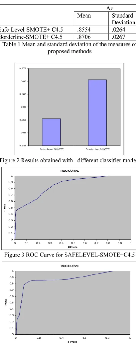
Before starting with the analysis, the results for the proposed methods in the experimental study are summarized in Table 1. Ten-fold cross-validation was performed and means and standard deviations of the metrics are reported. For more meaningful interpretation the classification results are summarized in the figure 2. Figure 3 and figure 4 show the ROC Curve for classifier models.
Two-tailed Student's t-tests at a level of significance of .05 were performed in order to compare the mean measure of two methods. A statistical comparison between the two methods yields a two-tailed p-value for rejecting / accepting the null hypothesis that their corresponding ROC curves have the same area under them. Statistical comparison between Safe-Level SMOTE+C4.5 and Borderline SMOTE + C4.5 yields a two-tailed p-value of 0.271 accepting the null hypothesis that their corresponding ROC curves have the same area under them.
Table 1 Mean and standard deviation of the measures of proposed methods
Figure 2 Results obtained with different classifier models
Figure 3 ROC Curve for SAFELEVEL-SMOTE+C4.5
Figure 4 ROC Curve for BORDERLINE-SMOTE+C4.5
0.845 0.85 0.855 0.86 0.865 0.87 0.875
Saf e- level SMOTE Bor der line SMOTE
ROC CURVE
0 0.1 0.2 0.3 0.4 0.5 0.6 0.7 0.8 0.9 1
0 0.1 0.2 0.3 0.4 0.5 0.6 0.7 0.8 0.9 1
FPrate
TP
ra
te
ROC CURVE
0 0.1 0.2 0.3 0.4 0.5 0.6 0.7 0.8 0.9 1
0 0.2 0.4 0.6 0.8 1
FPrate
TP
ra
te
Az Mean Standard
Deviation
Safe-Level-SMOTE+ C4.5 .8554 .0264
V
C
ONCLUSIONThe main focus of the paper is on improving the mass classification performance. It has been pointed out in the paper the major difficulties in the detection of masses. It has been highlighted why traditional classifiers are sensitive to the imbalanced data classification. Having identified the cause of problem with traditional classifiers some techniques have been proposed that can effectively handle the class imbalance problem for the classification of masses. Proposed method includes Safe-Level SMOTE + C4.5 and Borderline-SMOTE + C4.5. Quantitative evaluations are used to validate the effectiveness of proposed methods by ROC analysis. Two-tailed Student's t-tests at a level of significance of .05 were performed in order to compare the mean measure two methods. To evaluate proposed techniques, comparisons are carried out with many state of the art methods of mass detection and Borderline SMOTE + C4.5 outperforms other methods. Future works may focus on the integration of different classifier models
REFERENCES
[1] Wei D, Chan H.P, Helvie M.A, Shahiner B, Petrick N, and Alder
D.D, “Classification of Mass and Normal Breast Tissue on Digital Mammograms”, Med Physics, 22(9), 1501-13, Sept. 1995.
[2] Undrill P.E, Gupta R, and Henry S, “The Use of Texture Analysis
and Boundary Refinement to Delineate Suspicious Masses in Mammography”, SPIE, Medical Imaging: Image processing, SPIE 2710, 301-310, 1996.
[3] American Cancer Society, “Cancer Facts and Figures”, GA:
American Cancer Society, 2003.
[4] Mansees B S, “Evaluation of Breast Microcalcifications”, The
Radiologic Clinics of North America, Breast Imaging, Vol. 33, 6, 1109-1121, Jan 1995 .
[5] B.Surendiran, A.Vadivel, Henry Selvaraj, “A Soft-Decision
Approach for Microcalcification, Mass Identification from Digital Mammogram”, Proceedings of World Academy of Science, Engineering and Technology, volume 36 December, 2008.
[6] Roshan Dharshana Yapa and Koichi Harada, “Connected
Component Labeling Algorithms for Gray-Scale Images and Evaluation of Performance using Digital Mammograms”, IJCSNS International Journal of Computer Science and Network Security, Vol.8 No.6, June 2008.
[7] Grim, Petr Somol, Michal Haindl, and Jan Dane, “Computer-Aided
Evaluation of Screening Mammograms Based on Local Texture Models”, IEEE Transactions On Image Processing, Vol. 18, No. 4, April 2010.
[8] Jinshan Tang, Rangaraj M. Rangayyan, Jun Xu, Issam El Naqa, and
Yongyi Yang, ”Computer-Aided Detection and Diagnosis of Breast Cancer With Mammography: Recent Advances, IEEE Transaction On Information Technology In Biomedicine, Vol. 13, No. 2, March 2010.
[9] Arun Kumar M.N , and H.S. Sheshadri “Breast Contour Extraction
and Pectoral Muscle Segmentation in Digital Mammograms”, IJCSIS Vol. 9 No. 2, February 2011, (pp. 53-59).
[10] ICGST International Journal on Graphics, Vision and Image
Processing (GVIP) GVIP Special Issue on Mammograms, 2007
[11] Stelios Halkiotis, John Mantas & Taxiarchis Botsis. University of
Athens, Faculty of Nursing- Health Informatics Laboratory. “Computer-aided detection of clustered microcalcifications in digital mammograms”. 2000.
[12] B. Pataki, L. Lasztovicza “Extending Mammographic
Microcalcification Detection Method to Cluster Characterization”, Department of Measurement and Information Systems, Budapest University of Technology and Economics, Budapest, Hungary, 2008.
[13] Ranadhir Ghosh, Moumita Ghosh, John Yearwood, “A Modular
Framework for Multi category feature selection in Digital mammography”, ESANN'2004 proceedings - European Symposium on Artificial Neural Networks Bruges (Belgium), 28-30 April 2004. pp. 175-180.
[14] Sheshadri H.S, and Kandaswamy A, ―Detection of breast cancer
tumor based on morphological watershed algorithm‖, GVIP, 2005,
pp. 17-21.
[15] B. Verma, J. Zakos, “A computer-aided diagnosis system for digital
mammograms based on fuzzy-neural and feature extraction techniques”, IEEE Transaction on Biomedical. 5 (1) (2001) 46–54.
[16] I. El-Naqa, Y. Yang, M.N. Wernick, et al., “A support vector
machine approach for detection of microcalcifications”, IEEE Transaction on Medical Imaging 21 (12) (2002) 1552–1563.
[17] K.Thangavel and M.Karnan and R.Sivakumar and A. Kaja
Mohideen, "Ant Colony System for Segmentation and Classification of Microcalcification in Mammograms" GVIP Special Issue on Mammograms, 2007, pp.1-12
[18] S. Oporto-Dıaz, R. R. Hernandez-Cisneros and H. Terashima-Marn,
“Detection of microcalcification clusters in mammograms using a difference of optimized Gaussian filters”, in Proceedings of the Second International Conference on Image Analysis and Recognition, ICIAR 2005, Toronto, pp. 998–1005, 2005.
[19] Xue-wen Chen, Byron Gerlach, and David Casasent, “ Pruning
Support Vectors for Imbalanced Data Classification”, Proceedings of International Joint Conference on Neural Networks, Montreal, Canada, July 31 - August 4, 2005. 1
[20] Juanjuan Wang, Mantao Xu, Hui Wang, Jiwu Zhang,
“Classification of Imbalanced Data by Using the SMOTE Algorithm andLocally Linear Embedding”, ICSP2006 Proceedings. 2
[21] Xia Hong, “A Kernel-Based Two-Class Classifier for Imbalanced
Data Sets”, IEEE TRANSACTIONS ON NEURAL NETWORKS, VOL. 18, NO. 1, JANUARY 2007 8
[22] Alberto Fernández, María José del Jesus, Francisco Herrera,
“Hierarchical fuzzy rule based classification systems with genetic rule selection for imbalanced data-sets “,International Journal of Approximate Reasoning 50 (2009) 561–577. 16
[23] Nitesh V. Chawla, “C4.5 and Imbalanced Data sets: Investigating
the effect of sampling method, probabilistic estimate, and decision tree structure “, Workshop on Learning from Imbalanced Datasets II, ICML, Washington DC, 2003. 20
[24] Mu-Chen Chen a, Long-Sheng Chen, Chun-Chin Hsu, Wei-Rong
Zeng , “An information granulation based data mining approach for classifying imbalanced data “, Elsevier, Information Sciences 178 (2008) 3214–3227. 21
[25] Piyasak Jeatrakul, Kok Wai Wong, and Chun Che Fung, “ “,
“Classification of Imbalanced Data by Combining the Complementary Neural Network and SMOTE Algorithm”,
http://researchrepository.murdoch.edu.au 27.
[26] The mini-MIAS database of mammograms,