1
Temporal limits of visual motion processing: psychophysics
1and neurophysiology
23
Bart G. Borghuis1,5,*, Duje Tadin2,4, Martin J.M. Lankheet3,5, Joseph S. Lappin4,5, Wim A. van de 4
Grind5 5
6
1Department Anatomical Sciences and Neurobiology, University of Louisville School of Medicine,
7
Louisville, KY, USA.
8
2Brain and Cognitive Sciences, Center for Visual Science, Neuroscience, and Ophthalmology; University
9
of Rochester, Rochester, NY, USA
10
3Department of Animal Sciences, Wageningen University, Wageningen, Gelderland, The Netherlands
11
4Vanderbilt Vision Research Center, Vanderbilt University, Nashville, TN, USA
12
5Helmholtz Institute and Department of Functional Neurobiology, Utrecht University, Utrecht, The
13
Netherlands
14 15
*Corresponding author: [email protected]. 16
17
18 19
Abstract: Under optimal conditions, just 3-6 ms of visual stimulation suffices for humans to see motion.
20
Motion perception on this time scale implies that the visual system under these conditions reliably encodes,
21
transmits, and processes neural signals with near-millisecond precision. Motivated by in vitro evidence for
22
high temporal precision of motion signals in the primate retina, we investigated how neuronal and
23
perceptual limits of motion encoding relate. Specifically, we examined the correspondence between the
24
time scale at which cat retinal ganglion cells in vivo represent motion information and temporal thresholds
25
for human motion discrimination. The time scale for motion encoding by ganglion cells ranged from
4.6-26
91 ms, depended nonlinearly on temporal frequency but not on contrast. Human psychophysics revealed
27
that minimal stimulus durations required for perceiving motion direction were similarly brief, 5.6-65 ms,
28
similarly depended on temporal frequency but, above ~10%, not on contrast. Notably, physiological and
29
psychophysical measurements corresponded closely throughout (r = 0.99), despite more than a 20-fold
30
variation in both human thresholds and optimal time scales for motion encoding in the retina. These results
31
demonstrate that neural circuits for motion vision in cortex can maintain and make use of the high temporal
32
fidelity of the retinal output signals.
33 34 35
Keywords: human psychophysics; apparent motion; temporal integration; cat; retina; neural coding;
36
Hassenstein-Reichardt detector; model analysis
37 38
2
1. Introduction
39 40
It has been long known that the mammalian visual system is highly sensitive to motion, even when
41
presented briefly. For example, Exner [1] reported that when humans view two sequentially flashed stimuli,
42
the threshold for temporal order detection could be as short as 15 ms. Subsequent studies showed that under
43
optimal conditions even 3 - 6 ms temporal-order asynchrony can be reliably discriminated [2-4]. Under
44
these circumstances, the two stimuli are not perceived separately but as a single moving object (‘apparent
45
motion’), indicating that the percept involves visual motion processing.
46
The middle temporal visual area (area MT, or V5) is a region of extrastriate visual cortex in primates
47
that has been demonstrated to be critical for motion vision [5]. Area MT has among the shortest response
48
latencies in extrastriate cortex [6], consistent with the observation that human reaction times are shorter for
49
moving compared with stationary objects [7]. A short response latency is functionally meaningful because
50
it enables a rapid response to stimulus onset, for example, during collision avoidance. But appropriate
51
behavioral responses in a dynamic visual environment also require information about the stimulus – such
52
as the direction of motion – to be resolved at a high temporal rate [8]. Thus, there is a benefit to encoding
53
stimulus information on the briefest possible time scale.
54
Visual encoding starts in the retina, where visual transduction and signal processing within retinal
55
neural circuits culminates in selective encoding of the visual input by the ganglion cells. Ganglion cells
56
transmit visual information as series of action potentials (spike trains) through the optic nerve, via the lateral
57
geniculate nucleus (LGN) of the thalamus, to the visual cortex. The majority of ganglion cells in the retina
58
of cats and primates signal spatio-temporal changes in luminance contrast but do not, by themselves,
59
provide information about motion direction. Instead, current working models suggest that motion vision
60
depends on the integration of signals from multiple ganglion cells with spatially offset visual receptive
61
fields [9-12]. This is supported by computational analysis of population macaque retinal parasol-type
62
ganglion cell responses to a moving bar recorded in vitro, which showed that motion direction could be
63
reconstructed from temporal correlations in the cells’ spike trains at a time scale of 10–50 ms [13, 14].
64
Thus, the time scale at which ganglion cell spike train ensembles represent visual motion approaches the
65
inter-spike interval. This suggests that noise variations (variability) in neuronal spike timing may limit the
66
temporal fidelity of visual motion encoding [15, 16], but to what extent they do so has remained unclear.
67
Variability in neuronal spike timing is apparent from trial-to-trial variations in the times at which a cell
68
fires action potentials in response to repeated presentations of the same stimulus. Spike timing variability
69
stems from noise in neuronal signal transduction and transmission, and its demonstrated underlying sources
70
include quantal fluctuations in photon absorption, fluctuations in cyclic nucleotides within the
71
photoreceptors, as well as noise in ion channels and synaptic vesicle release [17]. For several of these
72
factors, the noise amplitude depends on stimulus parameters such as stimulus temporal frequency and
73
luminance contrast [18-21]. Here, we postulate that if spike timing variability limits the encoding of visual
74
motion information, then the time scale for resolving visual motion at the perceptual level should similarly
75
depend on these stimulus parameters. In agreement with this idea, model analysis of retinal ganglion cells
76
responses obtained from primate retina in vitro showed that the optimal time scale for decoding retinal
77
motion signals decreases with temporal frequency and contrast [13]. While other studies have explored the
78
relation between encoding accuracy at the neuronal and behavioral level for chromatic [22] and orientation
79
discrimination tasks [23], how the time scale of population motion encoding in the retina relates to the
80
temporal limits of visual motion perception remains unclear.
81
To address this, we assessed the relation between the time scale of motion encoding in mammalian
82
retinal ganglion cells in vivo and the temporal limits of human motion perception. We first recorded cat X-
83
and Y-type ganglion cell spike responses to motion stimuli with a range of contrasts and temporal
84
frequencies. We then used model analysis to compute from these responses, for each stimulus condition,
85
the time scale at which they best represent motion information. The measured time scales approximated
86
those reported for macaque parasol cells, supporting the assumption that the temporal precision of the
87
retinal spike output for a subset of ganglion cell types is similar across mammals. We then measured for
88
matched stimuli in humans the minimum stimulus duration required for motion direction discrimination.
3
We found that across stimuli, the temporal limit for visual motion discrimination at the perceptual level
90
closely matched the time scale of motion encoding at the ganglion cell level. Thus, it appears that human
91
motion perception adheres to the temporal fidelity of visual encoding at the level of the retinal ganglion
92
cells. Based on these results we conclude that the visual cortex both maintains and makes use of the
93
stimulus-dependent temporal fidelity of the retinal output for resolving visual motion.
94 95
2. Results
96 97
2.1 Electrophysiology and modeling
98 99
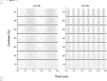
We recorded extracellular spike responses to repeated presentations of drifting sine wave gratings from 37
100
retinal ganglion cells (n = 33 X type, 4 Y type) from the optic tract and 20 visual relay cells (all X type)
101
from the lateral geniculate nucleus of anesthetized cats in vivo. Spatial frequency was optimized for each
102
cell, and temporal frequency and luminance contrast were varied (0.5 – 16 Hz; 10 - 70%). Increasing
103
contrast increased the modulation amplitude of a cell’s firing rate, as expected (Figure 1). We used the
104
recorded spike trains as input to a motion detector model to determine the time scale at which their temporal
105
structure represented motion information (see Methods for details).
106
The motion detector was modeled as a correlator in which input spike trains were first low-pass filtered
107
with a leaky integrator-type filter characterized by a time constant τ (Figure 2A) and then integrated. This
108
choice of filter was motivated by its simplicity and physiological relevance, as for a range of values of τ
109
the exponential tail can be interpreted as a first-order description of a receiving neuron's postsynaptic
110
potential [24]. Low-pass filtering transformed the spike train from a temporal point process with
time-111
varying rate into a continuous signal – a series of superimposed pulses with exponentially decaying tails.
112
Due to variability in spike timing, spikes in the two input spike trains rarely occurred within the same
113
0.5 ms spike acquisition time bin. Thus, for very small values of τ (<1 ms), cross-multiplication of the two
114
spike trains gave a near-zero output signal (Figure 2B). For large values of τ, on the other hand, the
115
correlator was largely insensitive to the timing of individual spikes, and its output reflected the mean
116
difference in firing rate [24], which was normalized in the model, so that for large τ, signal correlation
117
approached unity. Between these two extremes, correlation grew monotonically with the value of the time
118
constant (Figure 3).
119
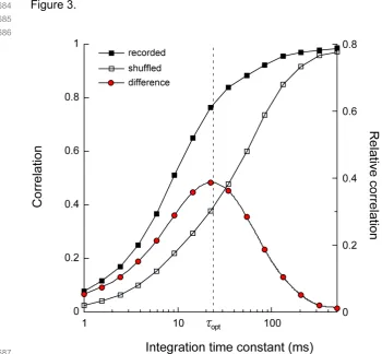
To determine how much motion information was carried by the temporal structure of the spike trains,
120
the procedure was repeated after randomly shuffling the inter-spike intervals in each spike train. This
121
eliminated temporal structure while preserving response statistics such as mean firing rate and the
inter-122
spike interval histogram. Again, correlation as a function of τ was a monotonic function (Figure 3).
123
However, shuffling shifted the curve towards larger τ, indicating that to obtain the same level of correlation
124
now required a longer integration time.
125
The shift shows that by discarding the temporal structure of the spike trains, motion information was
126
lost. Exactly how much information was lost is expressed by the difference between the original curve and
127
the shuffled response curve (Figure 3). This difference function peaked at an intermediate value of τ, about
128
23 ms in this example. At this integration time, the motion detector maximally extracts motion information
129
from the temporal structure of the input spike trains. We defined this value of τ as the optimal integration
130
time (τopt).
131
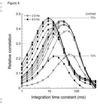
While temporal correlation between spike responses increased with increasing stimulus contrast, above
132
about 10%, contrast had very little effect on the optimal integration time (Figure 4). This was surprising,
133
considering the large apparent effect of contrast on spike timing variability (Figure 1). Instead, optimal
134
integration times depended strongly on temporal frequency: increasing temporal frequency caused
135
correlation curves to peak at shorter integration times. This effect was robust (~20-fold change across
136
presented frequency range) and was observed for all recorded cell types (retinal X, Y and LGN X-cells;
137
Figure 5).
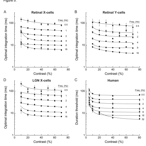
Retinal Y cells had the shortest optimal integration time, ranging from 79 ms at 0.5 Hz to 4.6 ms at 16
139
Hz (n = 4), indicating that these cells had the highest temporal fidelity. The optimal integration time for
140
retinal X cells was slightly longer, ranging from 91 ms at 0.5 Hz to 6.6 ms at 16 Hz (n = 33). The optimal
141
integration time for LGN X cells was slightly longer again, ranging from 113 ms at 0.5 Hz to 7.3 ms at 16
142
Hz. Optimal integration times for LGN X cell responses were on average 26.3 ± 13 % longer than those for
143
retinal X cells, suggesting some loss of temporal precision at the LGN-relay. Optimal integration times for
144
Y type retinal ganglion cells were on average 18.4 ± 7.8 ms shorter than for retinal X cell responses,
145
demonstrating greater temporal precision in Y-type cells.
146 147
2.2. Psychophysics
148 149
Across stimulus parameters, the time constant that maximized motion encoding in cat (above) approximated
150
values reported from primate retina [14], indicating that temporal fidelity may generalize across higher
151
mammals, including humans. If the optimal time constant for temporal integration reflects the time scale at
152
which retinal spike trains represent motion information, then presenting motion stimuli at shorter time
153
scales should impair cortical motion processing. Impaired cortical motion processing, in turn, should impair
154
psychophysical performance in a motion discrimination task. To test this, we next measured how human
155
motion discrimination depends on stimulus duration, and compared the minimum exposure duration
156
required for resolving motion direction at the perceptual level with the optimal integration times computed
157
from the output of the retina and LGN.
158
Duration thresholds [25] were measured for a direction discrimination task in which observers
159
discriminated motion (left vs. right) of a foveal Gabor stimulus. Stimulus size (0.33 deg at 2σ of the spatial
160
Gaussian envelope) approximated foveal V1 receptive field size (0.25 deg; [26], small enough to avoid
161
contrast dependent center-surround interactions reported for larger moving stimuli [27]. Spatial frequency
162
was optimized for the human fovea (3.0 c/deg; [28]. Contrast and temporal frequency - parameters known
163
to affect motion perception (e.g., [29-33] were systematically varied.
164
Psychophysical duration thresholds were very short, ranging from 5.6 ms at the highest temporal
165
frequency tested (32 Hz) to about 65 ms at 0.5 Hz. Across stimuli, duration thresholds closely matched the
166
optimal integration times computed from the responses of retinal X, Y and LGN cells (Figure 5A-D).
167
Optimal integration times computed from the electrophysiological data and human duration thresholds both
168
showed a robust dependence on temporal frequency that was largely independent of stimulus contrast.
169
Thresholds increased dramatically at combinations of low contrast (< ~10%) and high temporal frequency
170
(16 – 32 Hz). Because contrast sensitivity is known to decline strongly at high temporal frequencies [34]
171
these increased thresholds likely reflect impaired stimulus detection. To examine the correspondence
172
between the psychophysical and physiological results, we calculated asymptotic values of duration
173
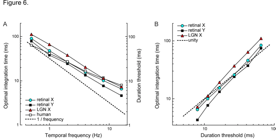
thresholds and τopt estimates at each temporal frequency (Figure 6). Asymptotic duration thresholds and τopt
174
estimates for different cell types were closely correlated (human vs. retinal X, r = 0.99; human vs. retinal
175
Y r =0.98; human vs. LGN X, r = 0.99; all p < 0.0001; Figure 7). Thus, duration thresholds and optimal
176
integration times show the same quantitative dependence on temporal frequency.
177
Finally, it is important to highlight that the observed dependency on temporal frequency cannot be
178
explained by the time it takes stimuli to cover a fixed proportion of its temporal cycle. This, arguably less
179
interesting explanation, would lead to proportionally shorter thresholds with increasing temporal frequency.
180
This was not the case. Expressed as a fraction of the stimulus cycle, human duration thresholds range from
181
1/5 of a cycle (4 arcmin) at 32 Hz to as little as 1/30 of a cycle (~ 0.7 arcmin) at 0.5Hz. This six-fold increase
182
in the threshold displacement rules out the hypothesis that threshold requires a fixed displacement of the
183
stimulus cycle. Analogously, if optimal integration times simply reflect the linear interaction between the
184
sine wave stimulus and the low pass filter of the detector model, we should expect a slope of 1 / frequency
185
(Figure 6A, dotted line). For all curves, the slope is significantly shallower (paired t-test; retinal X: p <
186
0.01; retinal Y: p = 0.087; LGN X: p = 0.016; human: p < 0.01) indicating that a proportionally smaller
187
stimulus period is required for direction discrimination at higher temporal frequencies. Thus, the
188
relationship between temporal frequency and both duration thresholds and τopt is non-linear. A likely
explanation is that at high temporal frequencies, temporal deviations in spike timing and unreliable spike
190
generation – where a cell may skip its spike response to a stimulus period – become predominant in the
191
response’s temporal structure, and disproportionately increase the optimal integration time compared with
192
lower temporal frequencies.
193 194
3. Discussion
195 196
For a range of stimulus parameters, we measured (1) the time scale at which a motion detector model
197
optimally detects motion from retinal ganglion cell responses and (2) the temporal threshold of human
198
motion perception. The time scales of motion encoding that we computed for cat closely match reported
199
values obtained from macaque retina, in vitro [14]. We found that across conditions, both the physiological
200
optimal integration time and the psychophysical temporal limit changed by more than 20-fold. This change
201
was non-linear with changes in temporal frequency and contrast. Importantly, over the entire range of
202
stimulus parameters, the two measurements were comparable: human duration thresholds and optimal
203
integration times showed a corresponding dependency on temporal frequency and contrast (Figures 5, 6).
204
This pattern of results is consistent with the hypothesis that spike timing variability, which affects the
205
optimal integration time, is an important factor limiting the temporal resolution of motion processing. Our
206
interpretation is that spike timing variability sets the shortest sequence of spikes that needs to be analyzed
207
by a motion detector to reliably signal motion, and that this temporal integration limits the minimum
208
stimulus exposure required for an observer to perceive motion direction. Note that the brief integration
209
times reported here are categorically different from the considerably longer temporal summation of motion
210
signal investigated elsewhere (e.g., Burr, 1981), which is thought to primarily reflect integration of neural
211
signals at stages downstream from motion detection. Our results show that the temporal limits of human
212
motion perception closely adhere to the time scale at which motion information is best extracted from
213
neuronal responses at the level of the retina and LGN, suggesting the high temporal fidelity of the retinal
214
input is maintained and utilized in visual cortex.
215 216
3.1. Comparison to other reports of motion acuity
217 218
Our lowest threshold (5.6 ms at 32 Hz) is comparable to the shortest temporal order judgments reported in
219
the literature, 3 – 6 ms [2-4]. It should be noted, however, that the stimuli used in previous studies
220
demonstrating hyperacuity for temporal order judgments were lines or circles, sequentially flashed at two
221
spatially separate locations. In each of these studies, total stimulus duration exceeded 10 ms. Our results
222
show that even briefer presentations suffice: drifting Gabor stimuli that are narrowband in both space and
223
time give similar temporal hyperacuity. Interestingly, psychophysical reports of temporal hyperacuity in
224
vision are generally restricted to stimuli with motion cues. When such cues are removed, temporal acuity
225
worsens to about 20-30ms [35, 36], which is comparable to the general temporal resolution of human vision
226
[37]. This suggests that the motion system has access to temporal fidelity that ius not available to other
227
visual sub-modalities.
228
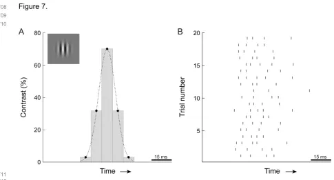
The brief psychophysical thresholds measured here and in earlier studies (less than 10 ms) imply that
229
motion direction can be computed from just a few spikes per cell. To illustrate this, Figure 7 shows
side-230
by-side the 16 Hz stimulus successfully discriminated by human observers (7.9 ms threshold; Figure 6) and
231
a retinal X cell’s response to one period of a drifting sine wave. A cell typically fired 3 to 4 spikes during
232
the time approximating the psychophysical stimulus presentation. For 32 Hz motion, which yielded the 5.6
233
ms psychophysical threshold, the number of spikes is even smaller. This suggests that for optimal stimuli,
234
motion direction can be computed from just a few spikes per retinal input. Such estimates, of course, are
235
likely to be noisy but can be improved by integrating responses from additional neurons [14]. This would
236
establish a trade-off between temporal acuity and spatial acuity.
237 238
3.2. Comparing electrophysiology to psychophysics
This study connects results derived from neurophysiological recordings in an in vivo animal model with
241
human psychophysical data – a link that should be treated with care [38]. To do so, it is important to consider
242
the underlying assumptions along with the experimental choices that were made, to determine the extent to
243
which the comparison of neurophysiological and psychophysical results was justified and meaningful.
244
First, we consider the assumptions behind neurophysiological recordings and accompanying modeling.
245
The relevance of these results depends on (1) the functional significance of the optimal integration times,
246
(2) the implications of mimicking pairs of cells with two responses from the same cell, and (3) the homology
247
of temporal limits in motion processing between cat and primates including humans.
248 249
3.3. Significance of the optimal integration time
250 251
Our model analysis of ganglion cell spike trains yields brief optimal integration times, and earlier work
252
showed feasibility of decoding spike trains on a similarly short time scale [13]. However, it not guaranteed
253
that the time scale over which the motion system integrates its inputs is, in fact, optimized for temporal
254
resolution. Indeed, a shorter-than-optimal integration time could result in attenuated, but nonetheless
255
significant detection (Figure 4), establishing a trade-off between signal-to-noise ratio, i.e. 'certainty', and
256
temporal resolution. Indeed, motion cortex may sacrifice signal-to-noise ratio to increase temporal
257
resolution: for example, longer, sub-optimal temporal integration could compensate for an apparent loss of
258
temporal resolution at the LGN X cell relay (Figure 6). Thus, while, τopt represents the time scale that would
259
enable a cell to maximize signal-to-noise ratio of the motion-evoked response, the actual parameters used
260
in cortical motion computation remain unclear – although our psychophysical results indicate they may be
261
similar. Finally, whether the time scale for encoding motion within a given neural circuit is fixed or whether
262
the same circuit can adapt its integration time depending on the task demands remains to be determined.
263 264
3.4. Use of single cells to model motion detector inputs
265 266
Spike train analysis was based on a common motion detector model, the bi-local correlator [39-41].
267
Essential to this, and most other motion-detection models, is the pair-wise correlation of signals from
268
spatially separate receptive fields after one input channel is delayed, typically through low-pass filtering
269
(Figure 2A). Here, we mimicked this mechanism by using two responses from the same cell, evoked by
270
repeated presentations of the same visual stimulus. This assumes that ganglion cells of the same type share
271
the same spatio-temporal response characteristics – an assumption that is supported by our experimental
272
results and those reported elsewhere [42, 43]. The benefit of using two responses from the same cell is that
273
this obviated the need to explicitly model a spatial separation and delay. Since the separation-delay
274
combination would be different for detectors tuned to different stimulus temporal frequencies (speeds), this
275
reduced the number of free parameters and simplified the model.
276
Hypothetical differences in the response characteristics of the cells that provide the correlator’s inputs
277
necessarily decrease the temporal correlation and, therefore, would require a longer integration time to
278
reach the same correlation coefficient. Because the response characteristics of cells in our model are
279
identical, the model gives an upper bound to the correlation coefficient and optimal integration time. With
280
increasingly dissimilar cells, this upper bound could still be approximated by pooling over a larger number
281
of inputs, and indeed, in macaque increasing the number of cells used in the computation of motion gives
282
a better overall performance [14].
283
Finally, our use of repeated responses from single cells assumes that ganglion cells have independent
284
noise, which is supported in the literature [44, 45]. While nearby retinal ganglion cells tend to fire correlated
285
spikes [46, 47], correlated neural activity only has a weak effect on the encoding of motion speed [14].
286
Together, these arguments should permit the use of single neuron recordings to approximate motion
287
encoding by two of more retinal inputs.
288 289
3.5. Species differences
We compared our results with those of Chichilnisky and Kalmar (2003), who employed an almost identical
292
bi-local detector model to compute optimal time scales for motion discrimination from ganglion cell
293
responses recorded in the macaque retina in vitro. For comparable stimuli, our estimates of optimal
294
integration times from cat X and Y-cells closely match the equivalent ‘optimal temporal filter widths’
295
reported for macaque parasol cells [13]. The optimal integration time for a cat retinal ganglion cell
296
responding to a sine wave drifting at 14 deg sec-1 is 12 ms. For macaque parasol cells responding to a bar
297
also moving at 14 deg sec-1, the optimal time scale reported by Chichilnisky and Kalmar (2003) is 13 ms.
298
This suggests that in terms of the time scale of motion encoding, cat X and Y and macaque parasol cells
299
are comparable.
300
The similarity between response temporal fidelity in cat and primate retina is perhaps not surprising
301
because variability in spike rate and spike timing is likely to be similar across these species. Response
302
variability at the level of the retina variability depends on four key factors: neural noise, contrast sensitivity,
303
refractory period, and peak firing rate. Because these are fundamental properties shared among equivalent
304
cell types (e.g., cat Y and primate parasol), one would not expect major differences between them, and none
305
have been reported. On the contrary, for a spatio-temporal white noise stimulus, cat and macaque retinal
306
responses appear to be highly similar (cat: [48-50]; macaque: [21, 42]. Thus, our measurements agree with
307
the established similarities of cat ganglion cell and macaque parasol cell responses. Because parasol cells
308
are thought to underlie motion vision in macaques and humans, the observed similarity also suggests that
309
measurements of responses in the front-end visual system in both cat and macaque can make valid
310
predictions for motion vision in humans.
311 312
3.6. Psychophysical assumptions
313 314
Finally, we considered the factors affecting psychophysical estimates of temporal limits in motion
315
perception. The results presented here are conditional on the definition of the stimulus duration and the
316
psychometric threshold. Moving stimuli were shown in a Gaussian temporal envelope, whose duration is,
317
in theory, infinite. In practice, duration is typically defined as 2σ of the temporal Gaussian (cf. [28], which
318
includes 68% of total stimulus contrast. Detection threshold was conservatively defined as 82% correct, a
319
commonly used optimal choice for a QUEST staircase [51]. Although our definition of the stimulus
320
duration and selection of the threshold level follow established conventions, they are arbitrary. When tested,
321
the use of other conventions resulted in small changes in duration threshold that did not affect our main
322
findings.
323
Psychophysical threshold can be affected by inadvertent slips of the subject’s attention, especially for
324
very brief stimuli. To prevent this, the delay between button press and stimulus onset was fixed and
325
therefore predictable for the subjects, who were experienced at the psychophysical task. The use of
326
adaptable staircases to measure thresholds further minimized any possible effects of inattention. The
327
remaining factors influencing psychophysical results are the task and the stimulus parameters. Here, the
328
task was the simplest possible discrimination task. Stimulus parameters were optimized for human motion
329
perception [28] and were designed to avoid known inhibitory effects of large moving stimuli [25].
330 331
Without direct physiological measurements of the neural correlate of the motion detector's integrator, we
332
can only infer the exact quantitative relationship between the temporal fidelity of the retina’s output and
333
the temporal limits of motion vision. Instead, we report here for closely matched stimulus conditions, strong
334
similarity and co-dependency on stimulus parameters between predicted optimal integration times and
335
human duration thresholds. Our findings support the hypothesis that the temporal limits of motion vision
336
approximate the limits set by motion encoding in the retina.
337 338
4. Methods
339 340
4.1. Electrophysiological preparation and recordings
Extracellular single unit recordings from retinal ganglion cells and LGN cells were obtained with tungsten
343
microelectrodes (TM33B20KT, World Precision Instruments, USA, typical impedance 2.0 MΩ at 1.0 kHz)
344
from 19 anesthetized adult cats of either sex (3 - 5 kg). Surgical procedures were standard and in accordance
345
with the guidelines of the Law on Animal Research of the Netherlands and of the Utrecht University's
346
Animal Care and Use Committee.
347
Anesthesia was induced by ketamine hydrochloride injection (Aescoket-plus, 20 mg kg-1, i.m.).
348
Following preparatory surgery, anesthesia was maintained by artificial ventilation with a mixture of 70%
349
N2O - 30% O2 and halothane (Halothaan, 0.4 - 0.7%). To minimize eye movements, muscle paralysis was
350
induced and maintained throughout the experiment by infusion of pancuronium bromide (Pavulon, 0.1 mg
351
kg-1 hr-1, i.v.). Oxygen-permeable contact lenses (+3.5 to +5 diopters, courtesy of NKL, Emmen, The
352
Netherlands) were used to both focus the visual stimulus on the retina and protect the corneae.
353
LGN and optic tract recordings were obtained at approximately 10 and 20 mm below the cortical
354
surface at Horsley-Clarke coordinates A8, L10 [52]. Action potentials from single cells were detected with
355
a window discriminator (BAK Electronics Inc.) and digitized at 2.0kHz (PCI 1200, National Instruments)
356
for on-line analysis and storage (Apple Macintosh G4 computer, custom-written software).
357 358
4.2. Visual stimulation
359 360
Stimuli for electrophysiology experiments were computer-generated (ATI rage graphics card, Macintosh
361
G4 computer, custom-written software), presented on a linearized 19", 100 Hz CRT monitor (Sony
362
Trinitron Multiscan 400PS) at 57 cm from the optic node and centered on the receptive field of the cell
363
under study. Mean luminance was 54 cd·m-2. For those cells (<15%) that showed significant response
364
modulation to the 100Hz refresh rate of the monitor [53], the frame rate was increased to 120Hz.
365
For each cell, spatial and temporal tuning curves were measured using drifting sinusoidal gratings
366
(spatial frequency 0.1 - 4.0 cycles deg-1, temporal frequency 0.5 – 50 Hz). Cells were classified as X or Y
367
on the basis of a null-test [54]. Responses to twenty repeats of a 3 second presentation of drifting sine wave
368
gratings were used for the model analysis. Sinusoidal gratings fully covered the receptive field and spatial
369
frequency was optimized for each cell (average 0.8 cycles deg-1). Temporal frequency and luminance
370
contrast were varied (0.5 – 16 Hz and from 10 - 70% Michelson contrast, respectively). A stimulus block
371
consisted of 6 temporal frequencies and 7 contrasts, resulting in 42 stimuli presented in a random order.
372
Data presented in this study were obtained from cells with receptive fields located within the central 15
373
degrees of the visual field. Only single unit recordings that were stable during at least 20 repeats of the
374
stimulus block and showed significant response modulation to the high contrast stimuli were accepted for
375 analysis. 376 377 4.3. Psychophysics 378 379
Stimuli for human psychophysics experiments were computer-generated using Matlab (The Mathworks;
380
Natick, MA), the Psychophysics Toolbox [55] and Video Toolbox [56], and shown on a linearized monitor
381
(800 x 600 pixels, 200 Hz). We used a bit stealing technique [57] to expand gray-scale resolution from 256
382
to 768 levels. To obtain a 200 Hz refresh rate, we used a high-speed PROCALIX monitor (Totoku, Irving,
383
TX) driven by a MP960 graphics card (VillageTronic, Berlin, Germany). Viewing was binocular at 83 cm
384
(yielding 2 x 2 arcmin per pixel). Luminance of the gray screen background was 41.1 cd/m2. Three
385
observers participated in the experiment (first and second authors and a naïve observer). All procedures
386
complied with institutionally reviewed guidelines for human subjects and all subjects provided written
387
informed content.
388
Stimuli were vertically oriented Gabor patches, comprising a drifting vertical sine grating windowed
389
by a stationary two-dimensional Gaussian envelope (2σ width = 20 arcmin, spatial frequency = 3
390
cycles/deg, starting phase randomized). Gabor contrast was modulated by a temporal Gaussian envelope.
391
Peak Gabor contrast and temporal frequency were varied in a 7 x 5 design (0.5 – 32 Hz and 5 – 80 %,
392
respectively). The observers’ task was to discriminate motion (left vs. right) of a briefly presented Gabor
patch. Duration thresholds [25, 58, 59] were estimated using two interleaved QUEST staircases [51], where
394
staircases adjusted the standard deviation of the temporal Gaussian envelope and converged to 82% correct.
395
Duration was defined as 2σ width of the Gaussian envelope. The entire set of 35 conditions was repeated
396
four times in random order. This yielded eight threshold estimates per condition, of which the first two
397
thresholds discarded as practice. Trials were self-paced. Each trial began with a key-press, followed by a
398
stimulus 350 ms later. Feedback was provided.
399
Given that we were expecting very brief motion direction thresholds (especially for high temporal
400
frequency conditions), we paid close attention to what is the lower limit of temporal stimulus duration that
401
we can accurately present and measure. Stimuli were displayed on a 200 Hz monitor by discrete sampling
402
of the temporal Gaussian waveform every 5 ms, while ensuring that the middle sample always contained
403
the peak of the Gaussian [59]. For example, a Gabor patch presented in a temporal Gaussian window with
404
2σ = 5.6 ms (our lowest threshold: 32 Hz motion, 80% peak contrast) would be shown in 3 video frames
405
displaying 20.1, 100, and 20.1% of the peak contrast (see Figure 7 for another example). To test for possible
406
floor effects at the highest stimulus temporal frequency (32 Hz) we measured duration thresholds for 8, 16,
407
and 32 Hz motion at 100 Hz and 200 Hz frame rates. Substantially lower thresholds for 8 and 16 Hz stimulus
408
presented at 200 Hz would indicate deleterious under-sampling of the Gaussian waveform at 100 Hz.
409
Respective thresholds for 8 and 16 Hz motion were 7.9% and 8.3% lower at 200 Hz than at 100 Hz frame
410
rate, likely indicating the effects of higher fidelity motion representation at 200Hz. In contrast, the threshold
411
for 32 Hz motion was 28% lower at 200 Hz, indicating a floor effect for 32 Hz motion at 100 Hz frame
412
rate. Based on these measurements, we can assert that our set up is adequate for measuring the 32 Hz
413
stimulus presented at a frame rate of 200 Hz.
414 415
4.4. Model analysis
416 417
Essential to most motion detection models is the integration of visual signals from spatially separated
418
receptive fields [39, 40]. Known as a bi-local motion detector (Figure 2A), the model’s output reflects the
419
time-varying correlation between the input signals, one of which is temporally delayed relative to the other
420
(Hassenstein and Reichardt, 1956). The delay causes sensitivity to the temporal sequence of stimulation of
421
the two receptive fields, and combined with a threshold nonlinearity renders its response selective for
422
motion direction. Because detector function is based on temporal correlations, motion detection depends
423
on temporal similarity of the input signals.
424
The input signals in our model are retinal spike trains. Their temporal correlation is determined by the
425
magnitude of noise variations (variability) in these spike patterns. If variability in the spike pattern is large
426
then the correlation between responses from the two cells will be small. Thus, variability in the cells’
427
temporal spike pattern should limit motion detection. The correlator can counter this variability, by
428
integrating the spike trains over a finite time window to increase temporal overlap. But temporal integration
429
comes at a cost of increasing the time scale at which motion may be resolved. To assess this trade-off, we
430
measured for the recorded ganglion cell responses how the integration time that optimizes correlation
431
detection varies with stimulus contrast and temporal frequency – parameters expected to affect ganglion
432
cell spike response variability.
433
The bi-local detector was modeled as a correlator unit whose two inputs signals were pairwise
434
combinations of spike trains recorded from a single ganglion cell, evoked by repeated presentation of the
435
same visual stimulus (minimum of 20 stimulus repeats; n = 33 retinal X cells, 4 retinal Y cells, and 20 LGN
436
X cells). Using responses on alternate trials obtained from a single cell simplifies the model, as it obviates
437
explicit modeling of spatial separation and time delay of the two input receptive fields, and maximizes
438
temporal correlations independent of temporal frequency. As such, the model represents a detector whose
439
input signals are spike responses from two cells with identical response characteristics and spatio-temporal
440
receptive fields, but subject to independent noise variations [44, 45]. Differences in response characteristics
441
and receptive fields between cells necessarily decrease temporal similarity of their spike responses –
442
resulting in poorer detection performance. Therefore, our model provides an upper limit to motion detector
443
performance given a ganglion cell’s spike response variability.
Input to the model was a set of recorded spike trains si(t), n ≥ 20,
445 446
(1) 𝑠 (𝑡) = ∑{ }𝛿(𝑡 − 𝑡 ); 𝑖 = 1, , , 𝑛.
447
448
Spike trains were passed through a first order filter with time constant τ, and normalized for τ, adding
449
an exponential tail with an integral of 1 to each spike,
450 451
(2) 𝑥 (𝑡, 𝜏) = 𝑠 (𝑡) ∗ 452
453
From this set, pairs of spike trains were multiplied, integrated and normalized to the integral of the first
454
spike train,
455 456
(3) 𝑦(𝜏) = ∙∑ ∑ ∙ ( , )∙ ( , )
( ) ∑ ∙ ( , )
457
458
This operation was performed for a series of τ ranging from 1 - 500 ms resulting in y(τ). Spike trains si(t)
459
were then shuffled by redistributing the inter-spike intervals in each spike train. This yields spike trains
460
si’(t) that have identical mean firing rates, yet lack all stimulus related temporal structure. Repeated for
461
shuffled spike trains si’(t), the same procedure results in y’(τ), which was used as a measure of chance-level
462
coincidence between spikes in the two the spike trains given the mean spike rate. The difference function
463
C(τ) describes the specific contribution of the temporal structure of the input spike trains to the coincidence
464
detected by the hypothetical correlator unit.
465 466
(4) 𝐶(𝜏) = 𝑦(𝜏) − 𝑦′(𝜏) 467
468
This simple motion model incorporates low-pass filtering (temporal integration) and correlation of
469
input signals — two essential components of established models of motion perception [39, 40, 60]. For
470
each cell and stimulus condition, all possible response pairs (180 minimum) were used in the simulations.
471
τopt was calculated by averaging the results from each spike train pair. Note that the actual procedure
472
followed was the closest possible numerical approximation (time base 0.5 ms) to the equations presented
473
here.
474 475 476
Acknowledgments: We thank Davis Glasser for help with manuscript preparation.
477 478
Author contributions: Conceptualization, B.G.B., D.T., M.J.M.L., J.S.L., and W.A.G.; Methodology,
479
B.G.B., D.T., and M.J.M.L.; Software, B.G.B., D.T., and M.J.M.L.; Validation, B.G.B., D.T., M.J.M.L.,
480
J.S.L., and W.A.G.; Formal Analysis, B.G.B. and D.T.; Investigation, B.G.B. and D.T.; Data Curation,
481
B.G.B. and D.T.; Resources, M.J.M.L., J.S.L., and W.A.G.; Writing—Original Draft Preparation, B.G.B.
482
and D.T.; Writing—Review & Editing, B.G.B., D.T., M.J.M.L., J.S.L., and W.A.G.; Visualization,
483
B.G.B. and D.T.; Supervision, M.J.M.L., J.S.L., and W.A.G.; Project Administration, J.S.L., and W.A.G.;
484
Funding Acquisition, M.J.M.L., J.S.L., and W.A.G.
485 486
Funding: This research was funded by NWO/ALW grant 805.04.134 (B.G.B, M.J.M.L.) and National
487
Institutes of Health grants EY028188 (B.G.B.).
488 489
Conflicts of Interest: The authors declare no conflict of interest.
References
493 494
1. Exner, S., Experimentelle Untersuchung der einfachsten psychischenProcesse: III. Abhandlung,
495
Der persönlichen Gleithung zweiter Teil. Pflügers Archiv für die gesamte Physiologie der
496
Menschen und der Thiere, 1875. 11: p. 403-432.
497
2. Sweet, A.L., Temporal discrimination by the human eye. American Journal of Psychology, 1953.
498
66: p. 185–198.
499
3. Wehrhahn, C. and D. Rapf, ON- and OFF-pathways form separate neural substrates for motion
500
perception: psychophysical evidence. J Neurosci, 1992. 12(6): p. 2247-2250.
501
4. Westheimer, G. and S.P. McKee, Perception of temporal order in adjacent visual stimuli. Vision
502
Res, 1977. 17(8): p. 887-92.
503
5. Born, R.T. and D.C. Bradley, Structure and function of visual area MT. Annu Rev Neurosci, 2005.
504
28: p. 157-189.
505
6. Schmolesky, M.T., et al., Signal timing across the macaque visual system. Child Abuse & Neglect,
506
1998. 22(6): p. 481-91.
507
7. Fairbank, B.A., Jr., Moving and nonmoving visual stimuli: a reaction time study. Percept Mot
508
Skills, 1969. 29(1): p. 79-82.
509
8. Buracas, G.T., et al., Efficient discrimination of temporal patterns by motion-sensitive neurons in
510
primate visual cortex. Neuron, 1998. 20(5): p. 959-69.
511
9. Elstrott, J. and M.B. Feller, Vision and the establishment of direction-selectivity: a tale of two
512
circuits. Curr Opin Neurobiol, 2009. 19(3): p. 293-7.
513
10. Lochmann, T., T.J. Blanche, and D.A. Butts, Construction of direction selectivity through local
514
energy computations in primary visual cortex. PLoS One, 2013. 8(3): p. e58666.
515
11. Peterson, M.R., B. Li, and R.D. Freeman, The derivation of direction selectivity in the striate cortex.
516
J Neurosci, 2004. 24(14): p. 3583-91.
517
12. Stanley, G.B., et al., Visual orientation and directional selectivity through thalamic synchrony. J
518
Neurosci, 2012. 32(26): p. 9073-88.
519
13. Chichilnisky, E.J. and R.S. Kalmar, Temporal resolution of ensemble visual motion signals in
520
primate retina. J Neurosci, 2003. 23: p. 6681-6689.
521
14. Frechette, E.S., et al., Fidelity of the ensemble code for visual motion in primate retina. J
522
Neurophysiol, 2005. 94: p. 119-135.
523
15. Borghuis, B.G., Spike timing precision in the visual front-end. 2003, Utrecht: Utrecht University
524
Library. 97-121.
525
16. Butts, D.A., et al., Temporal precision in the neural code and the timescales of natural vision.
526
Nature, 2007. 449(7158): p. 92-5.
527
17. Angueyra, J.M. and F. Rieke, Origin and effect of phototransduction noise in primate cone
528
photoreceptors. Nat Neurosci, 2013. 16(11): p. 1692-700.
529
18. Mainen, Z.F. and T.J. Sejnowski, Reliability of spike timing in neocortical neurons. Science, 1995.
530
268: p. 1503-1506.
531
19. Reid, R.C., J.D. Victor, and R.M. Shapley, The use of m-sequences in the analysis of visual
532
neurons: linear receptive field properties. Vis. Neurosci., 1997. 14(6): p. 1015-27.
533
20. Reinagel, P., Information theory in the brain. Curr Biol, 2000. 10: p. R542-R544.
534
21. Uzzell, V.J. and E.J. Chichilnisky, Precision of spike trains in primate retinal ganglion cells. J
535
Neurophysiol, 2004. 92(2): p. 780-9.
536
22. Hass, C.A., et al., Chromatic detection from cone photoreceptors to V1 neurons to behavior in
537
rhesus monkeys. J Vis, 2015. 15(15): p. 1.
538
23. Beaman, C.B., S.L. Eagleman, and V. Dragoi, Sensory coding accuracy and perceptual
539
performance are improved during the desynchronized cortical state. Nat Commun, 2017. 8(1): p.
540
1308.
541
24. van Rossum, M.C., A novel spike distance. Neural. Comput., 2001. 13(4): p. 751-63.
25. Tadin, D., et al., Perceptual consequences of center-surround antagonism in visual motion
543
processing. Nature, 2003. 424: p. 312-315.
544
26. Dow, B.M., et al., Magnification factor and receptive field size in foveal striate cortex of the
545
monkey. Exp. Brain Res., 1981. 44(2): p. 213-28.
546
27. Tadin, D., Suppressive mechanisms in visual motion processing: From perception to intelligence.
547
Vision Res, 2015. 115(Pt A): p. 58-70.
548
28. Watson, A.B. and K. Turano, The optimal motion stimulus. Vision Res., 1995. 35(3): p. 325-36.
549
29. Burr, D.C., Temporal summation of moving images by the human visual system. Proc. R. Soc. Lond.
550
B Biol. Sci., 1981. 211(1184): p. 321-39.
551
30. Burr, D.C. and B. Corsale, Dependency of reaction times to motion onset on luminance and
552
chromatic contrast. Vision Res., 2001. 41(8): p. 1039-48.
553
31. Edwards, M., D.R. Badcock, and S. Nishida, Contrast sensitivity of the motion system. Vision Res.,
554
1996. 36(16): p. 2411-21.
555
32. Nakayama, K. and G.H. Silverman, Detection and discrimination of sinusoidal grating
556
displacements. J. Opt. Soc. Am. A, 1985. 2(2): p. 267-74.
557
33. van de Grind, W.A., J.J. Koenderink, and A.J. van Doorn, Influence of contrast on foveal and
558
peripheral detection of coherent motion in moving random-dot patterns. J. Opt. Soc. Am. A, 1987.
559
4(8): p. 1643-52.
560
34. Burr, D.C. and J. Ross, Contrast sensitivity at high velocities. Vision Res, 1982. 22(4): p. 479-84.
561
35. Tadin, D., et al., High temporal precision for perceiving event offsets. Vision Res, 2010. 50(19): p.
562
1966-71.
563
36. Zanker, J.M. and J.P. Harris, On temporal hyperacuity in the human visual system. Vision Res,
564
2002. 42(22): p. 2499-508.
565
37. Kelly, D.H., Adaptation effects on spatio-temporal sine-wave thresholds. Vision Res, 1972. 12(1):
566
p. 89-101.
567
38. Teller, D.Y., Linking propositions. Vision Res, 1984. 24(10): p. 1233-46.
568
39. Barlow, H.B. and W.R. Levick, The mechanism of directionally selective units in rabbit's retina. J
569
Physiol, 1965. 178(3): p. 477-504.
570
40. Hassenstein, B. and W. Reichardt, Systemtheoretische Analyse der Zeit-, Reihenfolgen- und
571
Vorzeichenauswertung bei der Bewegungsperzeption des Russelkäfers Chlorophanus. Z.
572
Naturforsch., 1956. 11b: p. 513-525.
573
41. Reichardt, W., Autocorrelation, a principle for the evaluation of sensory information by the central
574
nervous system, in Sensory Communication, W.A. Rosenblith, Editor. 1961, MIT Press:
575
Cambridge, MA. p. 303-317.
576
42. Chichilnisky, E.J. and R.S. Kalmar, Functional asymmetries in ON and OFF ganglion cells of
577
primate retina. J Neurosci, 2002. 22(7): p. 2737-47.
578
43. Reinagel, P. and R.C. Reid, Precise firing events are conserved across neurons. J Neurosci, 2002.
579
22(16): p. 6837-41.
580
44. Croner, L.J., K. Purpura, and E. Kaplan, Response variability in retinal ganglion cells of primates.
581
Proc Natl Acad Sci U S A, 1993. 90: p. 8128-8130.
582
45. Ginsburg, K.S., J.A. Johnsen, and M.W. Levine, Common noise in the firing of neighbouring
583
ganglion cells in goldfish retina. J Physiol, 1984. 351: p. 433-450.
584
46. Mastronarde, D.N., Correlated firing of cat retinal ganglion cells. II. Responses of X- and Y-cells
585
to single quantal events. J Neurophysiol, 1983. 49(2): p. 325-49.
586
47. Mastronarde, D.N., Interactions between ganglion cells in cat retina. J Neurophysiol, 1983. 49(2):
587
p. 350-65.
588
48. Dan, Y., J.J. Atick, and R.C. Reid, Efficient coding of natural scenes in the lateral geniculate
589
nucleus: experimental test of a computational theory. J Neurosci, 1996. 16(10): p. 3351-62.
590
49. Keat, J., et al., Predicting every spike: a model for the responses of visual neurons. Neuron, 2001.
591
30(3): p. 803-17.
50. Reich, D.S., et al., Response variability and timing precision of neuronal spike trains in vivo. J
593
Neurophysiol, 1997. 77: p. 2836-2841.
594
51. Watson, A.B. and D.G. Pelli, QUEST: a Bayesian adaptive psychometric method. Percept.
595
Psychophys., 1983. 33(2): p. 113-20.
596
52. Reinoso-Suarez, F., Topographischer Hirnatlas der Katze. Translated edition by E. Merck AG,
597
Darmstad, Germany, 1961: p. T 24.
598
53. Eysel, U.T. and U. Burandt, Fluorescent tube light evokes flicker responses in visual neurons.
599
Vision Res, 1984. 24(9): p. 943-8.
600
54. Hochstein, S. and R.M. Shapley, Quantitative analysis of retinal ganglion cell classifications. J.
601
Physiol., 1976. 262(2): p. 237-64.
602
55. Brainard, D.H., The Psychophysics Toolbox. Spat. Vis., 1997. 10(4): p. 433-6.
603
56. Pelli, D.G., The VideoToolbox software for visual psychophysics: Transforming numbers into
604
movies. Spat. Vis., 1997. 10: p. 437-442.
605
57. Tyler, C.W., Colour bit-stealing to enhance the luminance resolution of digital displays on a single
606
pixel basis. Spat. Vis., 1997. 10(4): p. 369-77.
607
58. Murray, S.O., et al., Sex Differences in Visual Motion Processing. Curr Biol, 2018. 28(17): p.
2794-608
2799 e3.
609
59. Tadin, D., J.S. Lappin, and R. Blake, Fine temporal properties of center-surround interactions in
610
motion revealed by reverse correlation. J Neurosci, 2006. 26(10): p. 2614-22.
611
60. Adelson, E.H. and J.R. Bergen, Spatiotemporal energy models for the perception of motion. J. Opt.
612
Soc. Am. A, 1985. 2(2): p. 284-99.
Figure legends
615 616
Figure 1. Retinal ganglion cell responses to drifting sinusoidal grating stimuli. Raster plot of a 1 second
617
section of the response of a single retinal ganglion cell to drifting sinusoidal grating stimuli, varying in
618
contrast (10 - 70%) and temporal frequency (left 2.0; right 8.0 Hz). Each dot in the display represents a
619
spike. Each line represents the response to a single presentation of the stimulus. Stimuli were presented
620
randomly interleaved, and repeated a minimum of 20 times.
621 622
Figure 2. Temporal integration improves correlation detection. (A) Bilocal motion detector model.
623
Correlator unit X receives input from two units sampling the retinal image with spatially separated receptive
624
fields, RF1 and RF2. Through cross-multiplication of the input spike trains, the correlator's output is high
625
only when it receives positive input synchronously. The combination of spatial separation ∆x and temporal
626
delay ∆t in one of the input channels tunes the detector to stimulus motion with a velocity of ∆x/∆t. This
627
elementary model captures the essence of spatio-temporal correlation of the retinal input, a requirement for
628
any motion detection model. Because the correlator also responds to non-directional, uniform flicker,
di-629
rectional selectivity generally follows from a comparison of the output of two or more detectors, tuned to
630
opposite motion directions. (B) A short integration time (2 ms) gives little overlap between input signals 1
631
(top) and 2 (middle). Only highly coincident spikes (temporal deviation < ~4 ms) result in non-zero output
632
(bottom). (C) A long integration time (100 ms) gives substantial overlap between the two input signals and
633
results in a strong output signal (bottom).
634 635
Figure 3. Computing the optimal integration time. From the difference between the correlation curve
636
for the recorded (solid squares) and shuffled spike trains (open squares) we obtained a relative correlation
637
curve (red circles; see Model for details). We defined the optimal integration time (τopt) as the time constant
638
where the relative correlation curve peaks. At this integration time, the correlator best extracts motion
in-639
formation from the temporal structure of the input spike trains. Optimal integration times were computed
640
in Matlab, following cubic spline interpolation of the 15 data points.
641 642
Figure 4. Stimulus parameters set optimal integration time for correlation detection. Relative
corre-643
lation curves based on the data partially displayed in Figures 1 and 3. The optimal integration time
(inte-644
gration time at peak) decreases with increasing temporal frequency. Contrast (10 - 70%) determines total
645
correlation (peak height), but above about 10% has little effect on the optimal integration time.
646 647
Figure 5. Optimal integrations time and duration thresholds decrease with increasing temporal
fre-648
quency but change little with contrast. (A-C) Optimal integration times for all combinations of stimulus
649
temporal frequency and contrast for 33 retinal X cells, 4 retinal Y cells, and 20 LGN X cells. Optimal
650
integration time systematically decreased with increasing temporal frequency, but was largely independent
651
of contrast above about 10%. Error bars show mean ± SEM. (D) Minimal presentation duration required
652
for human observers to discriminate motion direction as a function of stimulus temporal frequency and
653
contrast. Duration threshold decreased with temporal frequency of the sinewave grating. Above about 10%,
654
duration threshold was largely independent of stimulus contrast. Error bars show mean ± SEM for four
655
subjects.
656 657
Figure 6. Optimal integration time closely matches duration threshold across stimulus conditions.
658
(A) Optimal integration times, averaged across responses to 40 - 70% contrast stimuli, decrease with
in-659
creasing temporal frequency. A similar decrease is observed for human duration thresholds. The slope of
660
each curve deviates systematically from 1/frequency (dotted line). Optimal integration time and duration
661
threshold do not simply reflect detection of a fixed stimulus displacement. (B) Optimal integration times
662
closely match duration thresholds, except at the highest temporal frequencies, where optimal integration
663
times for retinal Y cells are shorter than the duration threshold, i.e., their temporal fidelity exceeds
psycho-664
physical performance.
666
Figure 7. Direction discrimination apparently requires few spikes per cell. Human observers were
667
asked to discriminate motion direction of a drifting sine wave grating (16 Hz) in a spatial Gaussian envelope
668
(Gabor patch, top left). (A) Contrast of the Gabor patch was Gaussian modulated in time. Presented at 200
669
Hz, this paradigm allowed very brief presentations of stimulus motion. Example shows the discrete
sam-670
pling of contrast values (σ = 7.9 ms, 70% contrast). (B) To a drifting sine wave (16 Hz) of equivalent spatial
671
frequency and same contrast, a cat retinal ganglion cell fires ~4 spikes.
Figure 1.
674 675
Figure 2.
678 679 680
Figure 3.
684 685 686
Figure 4.
690 691 692
Figure 5.
696 697 698
Figure 6.
702 703 704
Figure 7.
708 709 710