Track reconstruction at LHC as a collaborative data challenge
use case with RAMP
SabrinaAmrouche1, Nils Braun2, Paolo Calafiura3, Steven Farrell3, Jochen Gemmler2, Cé-cile Germain4, Vladimir Vava Gligorov5, Tobias Golling1, Heather Gray3, Isabelle Guyon6, MikhailHushchyn7, VincenzoInnocente8, BalázsKégl9,10, SaraNeuhaus11, DavidRousseau9, AndreasSalzburger8, AndreiUstyuzhanin7,12, Jean-RochVlimant13, ChristianWessel14, and YetkinYilmaz9,10
1University of Geneva, Switzerland
2Karlsruhe Institute of Technology, Germany 3Lawrence Berkeley National Laboratory, CA, USA 4LAL and LRI, Orsay, France
5LPNHE, Paris, France
6LRI and Université Paris-Saclay, France
7Yandex School of Data Analysis (YSDA), Moscow, Russia 8CERN, Geneva, Switzerland
9LAL, Univ. Paris-Sud, CNRS/IN2P3, Université Paris-Saclay, Orsay, France 10Center for Data Science, Université Paris-Saclay, France
11Max Planck Institute for Physics, Munich, Germany 12Higher School of Economics (HSE), Moscow, Russia 13California Institute of Technology, CA, Germany 14University of Bonn, Germany
Abstract.Charged particle track reconstruction is a major component of data-processing in high-energy physics experiments such as those at the Large Hadron Collider (LHC), and is foreseen to become more and more challenging with higher collision rates. A simplified two-dimensional version of the track reconstruction problem is set up on a col-laborative platform, RAMP, in order for the developers to prototype and test new ideas. A small-scale competition was held during the Connecting The Dots/Intelligent Trackers 2017 (CTDWIT 2017) workshop. Despite the short time scale, a number of different ap-proaches have been developed and compared along a single score metric, which was kept generic enough to accommodate a summarized performance in terms of both efficiency and fake rates.
1 Data challenges and RAMP
Rapid Analytics and Model Prototyping (RAMP) [1] is an online data challenge platform, pri-marily motivated by the need to achieve a more systematic integration of the development. It aims to incorporate specific types of interactions between developers during the design process, and seeks insight into the evolution of the design. What distinguishes RAMP among various data challenge platforms is its focus on the progress rather than the result.
The RAMP includes many different types of data challenges, in addition to the track reconstruction challenge, to each of which any user can subscribe and submit several "solutions" for the formulated "problem". The problems can be of different types, such as classification, regression or clustering, in a variety of contexts such as chemistry, biology or climate research [1]. The distinguishing feature of RAMP is that the submission is the "code" to solve the problem, which runs remotely on a fully modularized workflow. For a given problem the users can implement methods for training and pre-dicting, with any level of intermediate processes, as long as the methods return the expected format for the prediction. A screenshot of the submission sandbox is shown in Figure 1. The submissions are written inpythonand can use common libraries such asnumpy[2],pandas[3],scikit-learn[4].
Figure 1. Screenshot of the RAMP sandbox window, with submission based on a basic DBSCAN clustering method [5]. Code submissions are made by either editing code on the page directly, or uploading the relevant files.
In order to test the code before submitting, the users are provided with a limited portion of the dataset that contains the relevant input and output columns, on which they can perform a quick cross-validation. The submitted code is then run in the backend to train and test on a larger dataset, and the results are displayed in an online table. Such modularization of the workflow allows the algorithms to be trained and tested on different datasets even after the data challenge, which will be the topic of the discussion in Section 6.
Taking into account the complexity of the track reconstruction problem and a short time period, the hackathon event during the CTDWIT 2017 workshop at LAL-Orsay started directly with the open phase in order to boost the first submission of the participants. This open phase also included a few test algorithms (without machine-learning techniques) as a guiding baseline.
2 Use case: Track reconstruction at the LHC experiments
Track reconstruction is one of the most important tasks in a high-energy physics experiment, as it provides high-precision position and momentum information of charged particles. Such informa-tion is crucial for a diverse variety of physics studies - from Standard Model tests to new particle searches - which require robust low-level information which can be further refined for a narrower and more specific physics context. Through the history of high-energy physics, there have been many different types of tracking detectors with very different design principles: from bubble chambers to time-projection chambers, from proportional counters to spark chambers, and more recently with sil-icon detectors... Although each of them have provided a different data topology, they all relied on the same principle: the small energy deposit of charged particles in well-defined locations, with particle trajectories being bent in an externally applied magnetic field. Future developments, like the High-Luminosity LHC [6, 7] which introduces a factor 10 increase in track multiplicity w.r.t. current LHC conditions, will make track finding very difficult.
A track reconstruction challenge [8] with a rather complete LHC detector simulation is being prepared by a number of co-authors and others. But for the limited time frame of this workshop, we propose a challenge where we reduce the track finding problem to two dimensions and emulate the topology of silicon detectors, such that there are few locations along the radius, and a very high precision along the azimuth. Such topology helps to simplify the track reconstruction problem to layer-by-layer azimuth determination, however, we hope to open room for further innovation as well.
3 Simulation
The challenge uses a simplified 2D detector model representative of an LHC detector with a toy model for particle generation and simulation, with sufficient complexity to make it non-trivial, with source code available in [9]. The detector consists of a plane with nine concentric circular layers with radii between 3.9 cm and 1 m, with a distribution typical of a full Silicon LHC detector. A homogeneous magnetic field of 2 Tesla perpendicular to the plane bends the charged particles so that a particle of momentumP (in MeV, with the conventionc = 1) has a circular trajectory of radiusR = 0P.3 (in millimeters). Layers have negligible thickness and each layer is segmented in azimuth with fine granularity. There are 2πR/pitchpixels in every layer, wherepitchis 0.025 mm for innermost layers 1-5 and 0.05 mm for outermost layers 6-9. Every "pixel" corresponds to the smallest detector unit defined by layer and azimuthal index.
A particle crossing a layer activates one pixel with a probability of 97%. The location of this activated pixel will be called ahitin the following. Since the detector has a very fine granularity in azimuth, the cases where two particles pass through a single pixel are rare (less than 0.2% probability). As a very simple simulation of hadronic interaction, a particle has a 1% probability to stop at each layer. Given all this, participants cannot assume a particle will leave a hit in each layer.
from a gaussian centered at zero and of widthσMS =13.6√x0/Pin radians. Thus trajectories devi-ate from perfect circular arcs. The energy loss is neglected, so that particles keep the same absolute momentum, hence the same local curvature, throughout the trajectory.
For each event, a Poisson distribution is sampled to determine the number of particles, with an average of 10 particles per event (3 orders of magnitude less than what is expected at HL-LHC). The particles are sampled uniformly in azimuth and momentum, with bounds on the momentum between 300 MeV and 10000 MeV. The lowest momentum is such that particles cannot loop in the detector. Each particle originates from a different vertex that is also randomly sampled from a normal distribution around the origin of width 0.667 mm, as a simple simulation of particles coming from B-hadrons orτ-leptons, so that particles cannot be assumed to come exactly from the origin. No additional random background hits have been simulated.
The data provided to the participant is one csv file with one line per hit corresponding to 10000 events, while a separate 10000 event file is kept private for the evaluation of the submissions by the RAMP platform. Hits are grouped per event in a random order. The following features are provided:
event number: arbitrary index, unique identifier of the event
particle number: arbitrary index, unique identifier of the ground truth particle having caused that hit. This number is hidden from the prediction method.
hit identifier: index of the hit in the event (implicit variable)
layer number: index of the layer where the hit occurs, from 1, the innermost layer, to 9, the outer-most layer
phi numberindex of the pixel corresponding to the hit, counting clockwise, from 0, atφ =0 to the maximum, which depend of the layer
x: horizontal coordinate of the hit
y: vertical coordinate of the hit
It should be noted that although one can easily translate layer and phi information into x and y (and vice versa), both are provided in order to help participants to gain time. The user code should return for each event of the test dataset a track number for each hit, the track number being an arbitrary unique (in the event) number corresponding to a cluster of hits.
4 Scoring
The programs of LHC experiments span a diverse range of physics topics, each with a different selec-tion and use of data. Although tracks are used in almost all analysis applicaselec-tions, they are employed in very different ways: sometimes as an important part of the signal, sometimes as an indicator of background. The overall goal of track reconstruction is to achieve the best correspondence between particles and tracks, where the term "particle" refers to the true particles and "track" refers to the in-formation deduced from the detector by the reconstruction algorithm. This correspondence is never perfect: Sometimes a particle is missed by the algorithm and this is referred to a lack ofefficiency, and sometimes a track is reconstructed out of a coincidental alignment of hits without corresponding to a genuine particle, which is referred to asfake.
best momentum resolution. Ultimately, the figure of merit is defined by the systematic uncertainty on the measured quantity which, as stated, varies for every study. It is therefore difficult to define in advance the perfect track reconstruction score that fits all.
Ultimately the score that was used in the hackathon was based on "fraction of hits that are correctly matched to a particle in a given event", and more precisely defined as follows:
1. Loop over particles to associate each particle to a set of tracks
2. Choose the track with the most hits in the particle, and associate it to the particle. The result will be many(track)-to-one(particle).
3. Loop over tracks and check which tracks are matched to the same particle.
4. In the case of multiple matching, remove all tracks (and their corresponding hits) from the list except the one with the most hits in the particle.
5. Count the number of remaining hits (that are all associated to tracks by construction), and divide it by the initial number of hits.
6. Assign the score of the event with the above, and average it over all the events.
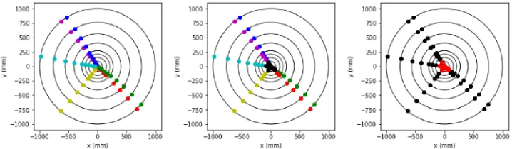
The code for the score function is provided to the participants as a part of the starting kit. Figure 2 illustrates the scoring procedure on a single event. Every event is scored separately, and the final result is averaged over events (all events having equal weight, regardless of number of hits).
Figure 2. Illustration of the scoring procedure. First plot shows the ground truth and the middle plot is the reconstructed output, after indices of tracks (represented by colors) are matched to the input. The black dots in the last plot shows the hits that are considered to be correctly assigned. For this particular event, the score is 0.81.
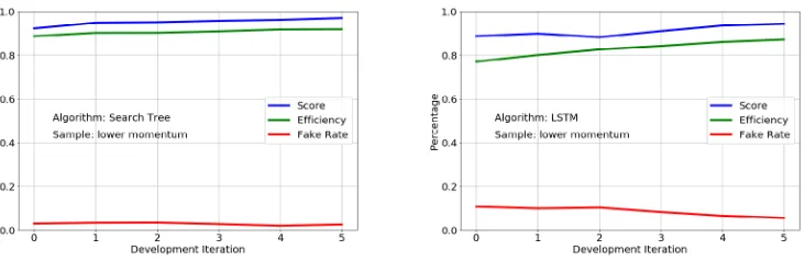
In Figure 3, several submissions for a specific algorithm are plotted, in which the participant only knows the score and tries to optimize that in every update. According to this study, an improvement in the score represents a monotonic improvement on both the efficiency and fake rate, therefore the score is reliable when upgrading the algorithms to achieve both better efficiency and less fakes. The robustness of the score function, in terms of efficiency and fake rate optimization in various samples, is further discussed in Section 6.
Figure 3. Illustration of the score as a performance indicator during the development process. Each panel corresponds to the submissions with a specific approach, incrementally being improved.
5 Example submissions
There were many interesting submissions during the hackathon, of which some with the highest scores are displayed in the leaderboard shown in Figure 4. At the end of the first day, the scores already started to approach towards a saturation around 97% as shown in Figure 5. Some of the approaches were totally independent, although some were a combination of existing baseline examples with im-proved features. We will now illustrate some of the example submissions which displayed interesting lines of development. The source code for these submissions can be accessed by signing up on the RAMP [1].
5.1 Untrained baseline examples
We started the hackathon with three baseline examples which we kept as simple as possible. These algorithms were not data-driven, therefore the training function was left blank.
Among these three, two algorithms were known to be only valid for the assumption that the cir-cular tracks have very small curvature and therefore can be approximated by straight lines. They all assumed the vertex position to be at the exact origin. In thelinear approximationalgorithm, the compatibility of hits with a straight line is tested and hits are clustered accordingly. In thenearest neighborsalgorithm, the hits at each next layer are matched to the closest hit in the previous layer.
Figure 4.Screenshot of the RAMP leaderboard, showing top 10 submissions as of March 9, 2017.
Figure 5. Development of algorithms during the hackathon. Although the submissions from the beta-testing period already had a high score, the participants were able to implement faster algorithms with even better scores.
Although the score of the Hough transform algorithm was one of the highest (0.97), it is slow (0.16s/event). The algorithms described below are faster, with similar scores.
5.2 TheΔφalgorithm
simple improvements allowed to increase the algorithm efficiency from 84% to 96% with small CPU performance degradation:
1. Allow tracks to have missing layers, including in the innermost and outermost layers;
2. Search for tracks bidirectionally: first outside-in, then inside-out;
3. Introduce a layer-dependent cut on direction vector alignment to take into account sensor pitch, and multiple scattering;
4. Follow the curvature of the track when comparing vector alignments, cutting on the difference between the currentCnand the running average<C>;
5. Allow hits to be shared among tracks, with a "sharing cost" tuned to limit fake tracks.
5.3 Inward search tree
The winning contribution (submitted ashyperbelle_tree) in the hackathon was inspired by a typical track reconstruction algorithm used in high energy physics, e.g. in the software currently developed for the Belle II experiment [10]. The implemented code is similar to a combinatoric Kalman filter and loosely based on the principles of a Monte Carlo Search Tree. To keep the implementation simple, the update step of the Kalman filter which, in real-world applications defines how well the algorithm works, was not implemented.
The algorithm starts with a random hit (the seed) on the outermost layer and builds up a tree using the hits on the next layer. A weight is calculated for each hit, which will be discussed below. Using only the hit with the maximal weight and those, which have a weight close to the maximal one, a new track candidate is built and the procedure is repeated until the innermost layer is processed.
The weight calculation is the crucial part in this algorithm. In this example implementation, the azimuthal angle difference between two successive hits is sampled on training data, where the truth information is known. From this histogrammed data, a probability for a given phi difference is extracted and used as a weight.
The tree search may produce multiple track candidates starting with the same seed hit, so only the candidate with the most consistency to a circle is stored. As there are no background hits, the tree search is continued until all hits of the event are assigned. To cope with hit inefficiencies, tracks which do not include hits of all layers are fitted together pairwise and tested for their fit quality. Good combinations are merged together.
As one part of the challenge was also to write fast algorithms, a runtime optimization of the imple-mentation was performed. Caching for the hits on each layer was implemented and heavy calculations and loops were realized usingnumpyfunctionality.
5.4 LSTM based algorithm
The LSTM submission [11] is based on a Long Short Term Memory neural network algorithm [12]. LSTMs can be powerful state estimators due to their effective usage of memory and non-linear mod-eling of sequence data. For this problem, the detector layers form the sequence of the model, and the predictions are classification scores of the hits for a given track candidate.
candidate at a time, so track "seeds" were identified using only the hits in the first detector layer. Each training sample input is prepared by using only the seed hit in the first layer plus all of the event’s hits in the remaining layers. The corresponding training sample target contains only the hits of the true track.
For each training sample, the LSTM model reads the input sequence and returns a prediction sequence for each corresponding detector layer. Each vector of the output sequence is fed through a fully connected neural network layer and a softmax activation function to give a set of "probability" scores over theφbins on that detector layer. For the bins that have hits in them, this score quantifies confidence that a hit belongs to the track candidate. The training objective, or cost function, is a categorical cross-entropy function.
Once trained, the model’s predictions can be used to assign labels to hits. Each event will contain a number of track candidates and thus each hit will have an associated score from the model predictions on each of those candidates. The assignment is made by choosing the candidate that gave the highest prediction score to the hit.
6 Tests with post-hackathon samples
As mentioned earlier, two of the baseline algorithms were only valid under the conditions of high average momentum and low detector occupancy. These algorithms are expected to fail if we test on a sample that moves out of these assumptions.
Some of the other algorithms, however, can learn the patterns and adapt to the conditions, if we also train on a sample that was prepared differently. This is how RAMP is set up, and here we illustrate the advantage of using the platform for the full analysis workflow rather than submitting a fixed solution.
In addition to the sample used in the hackathon (described in Section 3), we produced two alter-native samples which are more challenging in terms of the physics: lower momentum (more curved) tracks, and higher multiplicity (hence detector occupancy), summarized in Table 1.
Table 1.Parameters of the input samples.
sample multiplicity momentum range (MeV/c)
hackathon 10 [300,10000]
high-mult 20 [300,10000]
low-mom 10 [100,1000]
Since the linear approximation algorithm relies on the assumption that the tracks are almost straight lines, the algorithm starts to fail on a sample of tracks with more curvature. As shown in Figure 6, the test with high-multiplicity sample performs similarly to the hackathon sample, whereas the low-momentum sample displays a big degradation in the performance.
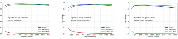
The Hough transform takes into account the curvature of the tracks, however it also displays (Figure 7) a slight degradation of performance in the high-multiplicity and low-momentum samples.
Performances of theΔφalgorithm (Figure 8) degrades slightly when going from the hackathon to the high-multiplicity sample, and significantly on the low-momentum sample due to difficulties accomodating the larger curvature of the tracks.
Figure 6.Performance of the linear approximation algorithm as a function of the angular window width, which is the only parameter of the algorithm. The left figure displays the performance in the nominal hackathon sample, the center and right figures display the performances in the modified "high-multiplicity" and "low-momentum" samples, respectively. The optimum window size highly depends on the momentum distribution.
Figure 7. Performance of the Hough transform algorithm as a function of the angular binning. The left figure displays the performance in the nominal hackathon sample, the center and right figures display the performances in the modified "high-multiplicity" and "low-momentum" samples, respectively. Although finer binning appears to almost monotonically increasing the efficiency, it may cause the loss of hits on the tracks, hence the score has slightly steeper dependence.
Figure 8. Performance of theΔφ algorithm as a function of the angular window width, which is the only parameter of the algorithm. The left figure displays the performance in the nominal hackathon sample, the center and right figures display the performances in the modified "high-multiplicity" and "low-momentum" samples, respectively. The optimum window size highly depends on the momentum distribution.
Figure 9.Performance of the inward search tree algorithm, as a function of the exponent of the cut applied on the weights. The left figure displays the performance in the nominal hackathon sample, the center and right figures display the performances in the modified "high-multiplicity" and "low-momentum" samples, respectively.
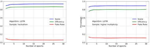
Figure 10.Performance of the LSTM algorithm as a function of number of epochs used in the training. The left figure displays the performance in the nominal hackathon sample and the right figure displays the performance in the modified "high-multiplicity" sample.
7 Conclusions and outlook
The problems for the CTDWIT 2017 hackathon were designed in a simplified way in 2D in order to allow the users to experiment on novel approaches, instead of being confined to regular methods of track reconstruction, within a 36 hours hackathon. In particular, the 2-dimensional setup simplified the visualisation of both the problem and solution, and the high average momentum and low multiplicity setup of the input samples made it easier to find a starting point for the development. With about 30 submissions in two days, the hackathon established a proof of principle for a wider scale data challenge for a more realistic experimental setup.
The post-hackathon test of the analysis in much more challenging physics conditions illustrated that it is possible to think ahead of the available data and implement robust solutions even if some features of the data are unknown. As expected, the algorithms that relied on the assumptions limited to the provided data failed, however a number of them maintained a high score. The experimental aspect of the hackathon was the observation of the contrasts of these approaches and their relative performances.
Acknowledgement
References
[1] Rapid analytics and model prototyping(2017),http://ramp.studio/
[2] S. van der Walt, S.C. Colbert, G. Varoquaux,The numpy array: A structure for efficient numeri-cal computation, computing in science&engineering(2011),http://www.numpy.org/
[3] W. McKinney, pandas : powerful python data analysis toolkit (2011),
http://pandas.sourceforge.net/
[4] F. Pedregosa, G. Varoquaux, A. Gramfort, V. Michel, B. Thirion, O. Grisel, M. Blondel, P. Pret-tenhofer, R. Weiss, V. Dubourg et al., Journal of Machine Learning Research12, 2825 (2011) [5] M. Ester, H.P. Kriegel, J. Sander, X. Xu,A density-based algorithm for discovering clusters in
large spatial databases with noise(AAAI Press, 1996), pp. 226–231
[6] The ATLAS Collaboration,CERN-LHCC-2015-020,"ATLAS Phase-II Upgrade Scoping Docu-ment"(2015)
[7] The CMS Collaboration, CERN-LHCC-2015-019,"CMS Phase-II Upgrade Scoping Document" (2015)
[8] The Tracking Machine Learning Challenge(2017),https://github.com/trackml
[9] TrackMLRamp Simulation (2017), https://github.com/ramp-kits/HEP_tracking/ tree/ramp_ctd_2017/simulation
[10] T. Abe et al. (Belle-II) (2010),arXiv:1011.0352
[11] S. Farrell,The HEP.TrkX Project: deep neural networks for HL-LHC online and offline tracking, inConnecting The Dots/Intelligent Trackers(2017)
![Figure 1. Screenshot of the RAMP sandbox window, with submission based on a basic DBSCAN clusteringmethod [5]](https://thumb-us.123doks.com/thumbv2/123dok_us/8134533.1355761/2.482.70.409.271.452/figure-screenshot-ramp-sandbox-window-submission-dbscan-clusteringmethod.webp)