Template Attacks on Different Devices

(1)

Template Attacks on Different Devices

Omar Choudary and Markus G. Kuhn

Computer Laboratory, University of Cambridge

firstname.lastname@cl.cam.ac.uk

Abstract. Template attacks remain a most powerful side-channel tech-nique to eavesdrop on tamper-resistant hardware. They use a profiling step to compute the parameters of a multivariate normal distribution from a training device and an attack step in which the parameters ob-tained during profiling are used to infer some secret value (e.g. crypto-graphic key) on a target device. Evaluations using the same device for both profiling and attack can miss practical problems that appear when using different devices. Recent studies showed that variability caused by the use of either different devices or different acquisition campaigns on the same device can have a strong impact on the performance of tem-plate attacks. In this paper, we explore further the effects that lead to this decrease of performance, using four different Atmel XMEGA 256 A3U 8-bit devices. We show that a main difference between devices is a DC offset and we show that this appears even if we use the same device in different acquisition campaigns. We then explore several variants of the template attack to compensate for these differences. Our results show that a careful choice of compression method and parameters is the key to improving the performance of these attacks across different devices. In particular we show how to maximise the performance of template attacks when using Fisher’s Linear Discriminant Analysis or Principal Component Analysis. Overall, we can reduce the entropy of an unknown 8-bit value below 1.5 bits even when using different devices.

Keywords:side-channel attacks, template attacks, multivariate analysis.

1 Introduction

Side-channel attacks are powerful tools for inferring secret algorithms or data (passwords, cryptographic keys, etc.) processed inside tamper-resistant hard-ware, if an attacker can monitor a channel leaking such information, most no-tably the power-supply current and unintended electromagnetic emissions.

(2)

an extensive study on 20 different devices, showing that the template attack may not work at all when the profiling and attack steps are performed on different devices; Elaabid et al. [14] showed that acquisition campaigns on the same device, but conducted at different times, also lead to worse template-attack results; and Lomn´e et al. [16] evaluated this scenario using electromagnetic leakage.

In this paper, we explore further the causes that make template attacks perform worse across different devices. For this purpose, we evaluate the template attacks with four different Atmel XMEGA 256 A3U 8-bit devices, using different compression methods and parameters.

We show that, for our experiments, a main difference across devices and ac-quisition campaigns is a DC offset, and this difference decreases very much the performance of template attacks (Section 4). To compensate for differences be-tween devices or campaigns we evaluate several variants of the template attack (Section 5). One of them needs multiple profiling devices, but can improve sig-nificantly the performance of template attacks when using sample selection as the compression method (Section 5.3). However, based on detailed analysis of Fisher’s Linear Discriminant Analysis (LDA) and Principal Component Analy-sis (PCA), we explain how to use these compression techniques to maximise the performance of template attacks on different devices, even when profiling on a single device (Section 5.4).

Overall, our results show that a good choice of compression method and pa-rameters can dramatically improve template attacks across different devices or acquisition campaigns. Previous studies [12,14] may have missed this by evalu-ating only one compression method.

2 Template Attacks

To implement a template attack, we need physical access to a pair of devices of the same model, which we refer to as the profiling and theattacked device. We wish to infer some secret valuek?∈ S, processed by the attacked device at some point. For an 8-bit microcontroller, S ={0, . . . ,255} might be the set of possible byte values manipulated by a particular machine instruction.

We assume that we determined the approximate moments of time when the secret value k? is manipulated and we are able to record signal traces (e.g., supply current or electromagnetic waveforms) around these moments. We refer to these traces as leakage vectors. Let{t1, . . . , tmr} be the set of timesamples andxr∈Rm

r

be the random vector from which leakage traces are drawn. During theprofiling phase we record npleakage vectorsxrki∈R

mr

from the profiling device for each possible valuek∈ S, and combine these as row vectors

xr

ki

0 _{in the leakage matrix}_Xr

k∈R np×mr_.1

Typically, therawleakage vectorsxr_kiprovided by the data acquisition device contain a very large numbermrof samples (random variables), due to high sam-pling rates used. Therefore, we might compress them before further processing,

1

(3)

either by selecting only a subset of m mr _{of those samples, or by applying}

some other data-dimensionality reduction method, such as Principal Component Analysis (PCA) or Fisher’s Linear Discriminant Analysis (LDA).

We refer to such compressed leakage vectors asxki∈Rm and combine all of these as rows into the compressed leakage matrixXk ∈Rnp×m_{. (Without any} such compression step, we would haveXk=Xrk andm=mr.)

Using Xk we can compute the template parameters ¯xk ∈ Rm and Sk ∈

Rm×m for each possible valuek∈ S as

¯

xk= _n1

p

np X

i=1

xki, Sk= _n1

p−1

np X

i=1

(xki−¯xk)(xki−¯xk)0, (1)

where the sample mean ¯xkand the sample covariance matrixSkare the estimates

of the true meanµk and true covarianceΣk. Note that

np X

i=1

(xki−x¯k)(xki−x¯k)0=Xe0_kXek, (2)

where Xek isXk with ¯x0k subtracted from each row, and the latter form allows

fast vectorised computation of the covariance matrices in (1).

In our experiments we observed that the particular covariance matricesSk

are very similar and seem to be independent of the candidatek. In this case, as explained in a previous paper [17], we can use a pooled covariance matrix

Spooled=

1

|S|(np−1)

X

k∈S

np X

i=1

(xki−x¯k)(xki−x¯k)0, (3)

to obtain a much better estimate of the true covariance matrixΣ.

In theattack phase, we try to infer the secret valuek?∈ S processed by the attacked device. We obtainnaleakage vectorsxi∈Rmfrom the attacked device, using the same recording technique and compression method as in the profiling phase, resulting in the leakage matrix Xk? ∈ Rna×m. Then, using Spooled, we

can compute a linear discriminant score [17], namely

djoint_LINEAR(k|Xk?) = ¯x0kS

−1 pooled

X

xi∈Xk? xi

−na

2 x¯

0

kS

−1

pooled¯xk, (4)

for eachk∈ S, and try allk∈ S on the attacked device, in order of decreasing score (optimized brute-force search, e.g. for a password or cryptographic key), until we find the correctk?.

2.1 Guessing Entropy

In this work we are interested in evaluating the overall practical success of the template attacks when using different devices. For this purpose we use the

(4)

brute-force search. The guessing entropy gives the expected number of bits of uncertainty remaining about the target valuek?, by averaging the results of the attack over allk?∈ S. The lower the guessing entropy, the more successful the attack has been and the less effort remains to search for the correctk?. We com-pute the guessing entropygas shown in our previous work [17]. For all the results shown in this paper, we compute the guessing entropy on 10 random selections of tracesXk? and plot the average guessing entropy over these 10 iterations.

2.2 Compression Methods

Previously [17], we provided a detailed comparison of the most common compres-sion methods: sample selection (1ppc, 3ppc, 20ppc, allap), Principal Component Analysis (PCA) and Fisher’s Linear Discriminant Analysis (LDA), which we summarise here. For the sample selection methods 1ppc, 3ppc, 20ppc and allap, we first compute a signal-strength estimates(t) for each samplej∈ {1, . . . , mr}, by summing the absolute differences2_{between the mean vectors ¯}_xr

k, and then

se-lect the 1 sample per clock cycle (1ppc, 6≤m≤10), 3 samples per clock cycle (3ppc , 18 ≤ m ≤ 30), 20 samples per clock cycle (20ppc, 75 ≤ m ≤ 79) or the 5% samples (allap, m = 125) having the largest s(t). For PCA, we first combine the first m eigenvectors uj ∈ Rm

r

of the between-groups ma-trix B =P

k∈S(¯xrk−x¯

r_)(¯_xr

k−x¯

r₎0_, _{where ¯}_xr ₌ 1

|S|

P

k∈Sx¯rk, into the matrix

of eigenvectors U = [u1, . . . ,um], and then we project the raw leakage

matri-ces Xr_k into a lower-dimensional space as Xk = XrkU. For LDA, we use the

matrix B and the pooled covariance Spooled from (3), computed from the

un-compressed traces xr

i, and combine the eigenvectors aj ∈Rm r

ofS−_pooled1 B into

the matrixA= [a1, . . . ,am]. Then, we use the diagonal matrixQ∈Rm×m, with

Qjj = (aj0Spooledaj)−

1

2,to scale the matrix of eigenvectorsAand useU=AQ to project the raw leakage matrices asXk =XrkU. In this case, the compressed

covariances Sk ∈Rm×m andSpooled ∈ Rm×m reduce to the identity matrixI, resulting in more efficient template attacks.

For most of the results shown in Sections 4 and 5, we used PCA and LDA with m= 4, based on the elbow rule (visual inspection of eigenvalues) derived from a standard implementation of PCA and LDA. However, as we will then show in Section 5.4, a careful choice ofmis the key to good results.

2.3 Standard Method

Using the definitions from the previous sections, we can define the following

standard method for implementing template attacks.

Method 1 (Standard)

1. Obtain the npleakage traces inXk from the profiling device, for each k.

2. Compute the template parameters(¯xk,Spooled)using (1,3).

3. Obtain the leakage tracesXk? from the attacked device.

4. Compute the guessing entropy as described in Section 2.1.

2

(5)

3 Evaluation Setup

For our experimental research we produced four custom PCBs (named Alpha,

Beta,Gamma andDelta) for the unprotected 8-bit Atmel XMEGA 256 A3U

mi-crocontroller. The current consumption across all CPU ground pins is measured through a single 10-ohm resistor. We powered the devices from a battery via a 3.3 V linear regulator and supplied a 1 MHz sine wave clock signal. We used a Tektronix TDS 7054 8-bit oscilloscope with P6243 active probe, at 250 MS/s, with 500 MHz bandwidth in SAMPLE mode. Devices Alpha and Beta used a CPU with week batch ID 1145, while Gamma and Delta had 1230.

For the analysis presented in this paper we run five acquisition campaigns: one for each of the devices, which we call Alpha, Beta,Gamma and Delta (i.e. the same name as the device), and another one at a later time for Beta, which we

call Beta Bis. For all the acquisition campaigns we used the settings described

above. Then, for each campaign and each candidate value k ∈ {0, . . . ,255} we recorded 3072 tracesxr

ki(i.e., 786 432 traces per acquisition campaign), which we

randomly divided into atraining set (for the profiling phase) and anevaluation

set (for the attack phase). Each acquisition campaign took about 2 hours. We note a very important detail for our experiments: instead of acquiring all the traces per k sequentially (i.e. first the 3072 traces fork = 0, then 3072 traces fork= 1, and so on), we used random permutations of all the 256 valueskand acquired 256 traces at a time (corresponding to a random permutation of all the 256 valuesk), for a total of 3072 iterations. This method distributes equally any external noise (e.g. due to temperature variation) across the traces of all the values k. As a result, the covariances Sk will be similar and the mean vectors

¯

xk will be affected in the same manner so they will not be dependent on factors

such as low-frequency temperature variation.

For all the results shown in this paper we used np = 1000 traces xrki per

candidate k during the profiling phase. Each trace contains mr _{= 2500}

sam-ples, recorded while the target microcontroller executed the same sequence of instructions loaded from the same addresses: a MOV instruction, followed by several LOAD instructions. All the LOAD instructions require two clock cycles to transfer a value from RAM into a register, using indirect addressing. In all the experiments our goal was to determine the success of the template attacks in recovering the byte kprocessed by the second LOAD instruction. All the other instructions were processing the value zero, meaning that in our traces none of the variability should be caused by variable data in other nearby instructions that may be processed concurrently in various pipeline stages. This approach, also used in other studies [8,13,17], provides a general setting for the evaluation of the template attacks. Specific algorithm attacks (e.g. on the S-box output of a block cipher such as AES) may be mounted on top of this.

4 Ideal vs Real Scenario

(6)

100 101 102 103 0

1 2 3 4 5 6

na(log axis)

Guessing entropy (bits)

LDA, m=4 PCA, m=4 sample, 1ppc sample, 3ppc sample, 20ppc sample, allap

100 101 102 103 0

1 2 3 4 5 6

na(log axis)

100 101 102 103 0

1 2 3 4 5 6

na(log axis)

100 101 102 103 0

1 2 3 4 5 6

na(log axis)

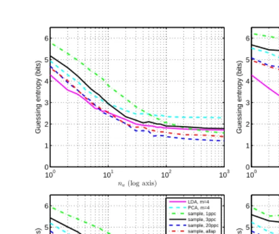
Fig. 1. Template attacks using Method 1 in different scenarios. Top-left (ideal): using same device and acquisition campaign (Beta) for profiling and attack. Top-right: using

Alpha for profiling andBeta for attack. Bottom-left: arithmetic average of guessing

entropy over all combinations of different pairs of devices for profile and attack. Bottom-right: using same device (Beta) but different acquisition campaigns for profile (Beta) and attack (Beta Bis).

in their evaluation. The results of the standard Method 1 in this ideal case, where we used the same acquisition data for profiling and attack (but disjoint sets of traces), are shown in Figure 1 (top-left). We can see that most compression methods perform very well for large na, while for smaller na LDA is generally

the best. This is in line with our previous results [17].

However, in a more realistic scenario, an attacker who wants to infer some secret data from a target device may be forced to use a different device for profiling. Indeed, there are situations where we could use non-profiled attacks, such as DPA [1], CPA [3], or MIA [9], to infer secret data using a single device (e.g. by targeting values that represent a known relationship between key and plaintext). But these methods cannot be used in more general situations where we want to infer a single secret data value that does not depend on any other values, which is the setting of our experiments. In such cases the template attacks or the stochastic approach [4] might be the only viable side-channel attack.3

3 _{In our setting we cannot use the non-profiled stochastic method (termed}_on-the-fly

(7)

Moreover, the template attacks are expected to perform better than the other attacks when provided with enough profiling data [11]. Therefore, we would like to use template attacks also with different devices for profiling and attack.

As we show in Figure 1 (top-right), the efficacy of template attacks using the standard Method 1 drops dramatically when using different devices for the profiling and attack steps. This was also observed by Renauld et al. [12], by testing the success of template attacks on 20 different devices with 65 nm CMOS transistor technology. Moreover, Elaabid et al. [14] mentioned that even if the profiling and attack steps are performed on the same device but on different acquisition campaigns we will also observe weak success of the template attacks. In Figure 1 (bottom-right) we confirm that indeed, even when using the same device but different acquisition campaigns (same acquisition settings), we get results as bad or even worse as when using different devices. In Section 5, we offer an explanation for why LDA can perform well across different devices.

4.1 Causes of trouble

In order to explore the causes that lead to worse attack performance on different acquisition campaigns, we start by looking at two measures of standard deviation (std), that we callstd devices andstd data.

Let ¯x(_kji) be the mean value of sample j ∈ {1, . . . , m} for the candidate

k ∈ S on the campaign i ∈ {1, . . . , nc}, ¯x (i)

j =

1

|S|

P

k∈Sx¯

(i)

kj, zk(j) = [(¯x

(1)

kj −

¯

x(1)_j ), . . . ,(¯x(nc)

kj −x¯

(nc)

j )] = [z

(1)

k (j), . . . , z

(nc)

k (j)] and ¯zk(j) =

1

nc Pnc

i=1z (i)

k (j).

Then,

std devices(j) = 1

|S|

X

k∈S

v u u t

1 nc−1

nc X

i=1

(z_k(i)(j)−z¯k(j))

2

, (5)

and

std data(j) = 1 nc

nc X

i=1

s 1

|S| −1 X

k∈S

(¯x(_kji)−x¯(_ji))2. (6)

We show these values in Figure 2. The results on the left plot are from the four campaigns on different devices, while the results on the right plot are from the two campaigns on the device Beta. We can observe that both plots are very similar, which suggests that the differences between campaigns are not entirely due to different devices being used, but largely due to different sources of noise (e.g., temperature, interference, etc.) that may affect in a particular manner each acquisition campaign. Using a similar type of plots, Renauld et al. [12, Fig. 1] observed a much stronger difference, attributed to physical variability. Their observed differences are not evident in our experiments, possibly because our devices use a larger transistor size (around 0.12µm)4_.

4

(8)

850 900 950 0

Sample index

std devices std data clock

850 900 950

0

Sample index

std devices std data clock

Fig. 2. std devices(j) andstd data(j), along with clock signal for a selection of samples around the first clock cycle of our target LOAD instruction. Left: using the 4 campaigns on different devices. Right: using Beta and Beta Bis.

850 878 884 900 950

−0.3 −0.2 −0.1 0 0.1 0.2

Sample index

Milliamps

Alpha Beta Beta bis Gamma Delta Beta + ci Beta − ci SNR of Beta

Fig. 3. Overall mean vectors ¯xfor all campaigns, from which the overall mean vector of Beta was substracted.Beta+ciandBeta−cirepresent the confidence region (α= 0.05) for the overall mean vector of Beta.SNR of Betais the Signal-to-Noise signal strength estimate of Beta (rescaled). Samples at first clock cycle of target LOAD instruction.

4.2 How it differs

Next we look at how the overall power consumption differs between acquisition campaigns. In Figure 3, we show the overall mean vectors ¯x= _|S|1 P

k∈Sx¯k for

each campaign, from which we removed the overall mean vector of Beta (hence the vector for Beta is 0). From this figure we see that all overall mean vectors ¯x

(9)

It is clear from Figure 3 that a main difference between the different cam-paigns is an overall offset. We see that this is also the case over the samples corresponding to the highest SNR. If we now look at the distributions of our data, as shown in Figure 4 for Alpha and Beta, we observe that the distribu-tions are very similar (in particular the ordering of the different candidateskis generally the same) but differ mainly by an overall offset. This suggests that, for our experiments, this offset is the main reason why template attacks perform badly when using different campaigns for the profiling and attack steps.

3.2 3.4 3.6 3.8 4 4.2 4.4 4.6 4.8 5 0

0.5 1 1.5 2 2.5

Milliamps

0 1 2 3 4 5 6 7 8 9

3.2 3.4 3.6 3.8 4 4.2 4.4 4.6 4.8 5 0

0.5 1 1.5 2 2.5

Milliamps

0 1 2 3 4 5 6 7 8 9

Fig. 4. Normal distribution at sample indexj= 884 based on the template parameters (¯xk,Spooled) fork∈ {0,1, . . . ,9}. Left: on Alpha. Right: on Beta.

4.3 Misalignment

We also mention that in some circumstances the recorded traces might be mis-aligned, e.g. due to lack of a good trigger signal, or random delays introduced by some countermeasure. In such cases, we should first apply a resynchronisation method, such as those proposed by Homma et al. [7]. In our experiments we used a very stable trigger, as shown by the exact alignments of sharp peaks in Figure 3.

5 Improved attacks on different devices

In this section, we explore ways to improve the success of template attacks when using different devices (or different campaigns), in particular by dealing with the campaign-specific offset noted in Section 4. We assume that the attacker can profile well a particular device or set of devices, i.e. can get a large number np

of traces for each candidate k, but needs to attack a different device for which he only has access to a set of na traces for a particular unknown target value

(10)

5.1 Profiling on Multiple Devices

Renauld et al. [12] proposed to accumulate the sample means ¯xk and variances

Sjj (where S can be either Sk or Spooled) of each sample xj across multiple

devices in order to make the templates more robust against differences between different devices. That is, for each candidate k and sample j, and given the sample means ¯xk and covariancesSfromnc training devices, they compute the

robust sample means ¯x(robust)_kj = 1

nc(¯x

(1)

kj +. . .+ ¯x

(nc)

kj ) (i.e. an average over the

sample means of each device), and the robust variance as S_jj(robust) = S_jj(1)+

1

nc−1

nc X

i=1

(¯x(_kji)−x¯(robust)_kj )2 (i.e. they add the variance of one device with the

variance of the noise-free sample mean across devices, using simulated univariate noise for each device). However, this approach does not consider the correlation between samples or the differences between the covariances of different devices. Therefore, we instead use the following method, where we use the traces from all available campaigns.

Method 2 (Robust Templates from Multiple Devices)

1. Obtain the leakage tracesX(_ki)from each profiling devicei∈ {1, . . . , nc}, for

eachk.

2. Pull together the leakage traces of each candidate kfrom all nc devices into

an overall leakage matrixX(robust)_k ∈Rnpnc×m _{composed as}

X(robust)_k 0= [X(1)_k 0, . . . ,X(nc)

k

0

]. (7)

3. Compute the template parameters(¯xk,Spooled)using (1,3) onX

(robust)

k .

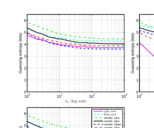
In our evaluation of Method 2, we used the data from the campaigns on the four devices (Alpha, Beta, Gamma, Delta), by profiling on three devices and attacking the fourth. The results are shown in Figure 5. We can see that, on average, all the compression methods perform better than using Method 1 (Figures 1 and 5, bottom-left). This is because, with Method 2, the pooled covariance Spooled captures noise from many different devices, allowing more

variability in the attack traces. However, the additional noise from different devices also has the negative effect of increasing the variability of each leakage sample [12, Fig. 4]. As a result, we can see that for the attacks on Beta, LDA performs better when we profile on a single device (Alpha) than when we use three devices (Figures 1 and 5, top-right).

5.2 Compensating for the Offset

(11)

100 101 102 103 0

1 2 3 4 5 6

na(log axis)

100 101 102 103 0

1 2 3 4 5 6

na(log axis)

100 101 102 103 0

1 2 3 4 5 6

na(log axis)

100 101 102 103 0

1 2 3 4 5 6

na(log axis)

Fig. 5. Results of Method 2, profiling on three devices and attacking the fourth one. Top-left: attack on Alpha; top-right: attack on Beta; bottom-left: arithmetic average of guessing entropy over all four combinations; bottom-right: attack on Delta.

we expect that a template attack that removes this offset should provide better results. Elaabid et al. [14] have shown that, indeed, if we replace each trace from each campaign by the difference between itself and the overall mean ¯x of that campaign (they refer to this process asnormalisation, and this process may also include division by the overall standard deviation), we can obtain results very similar to those in the ideal case (profiling and attack on the same campaign). However, this approach does not work straight away in a more realistic scenario in which the attacker only has access to a limited number of traces from the target device for a particular target valuek?, and hence he cannot compute the overall mean ¯x of the campaign. Nevertheless, if the difference between campaigns is mainly a constant overall offset (as we showed in Section 4.2), then an attacker may still use the subset of available attack tracesXk? to improve the template

attack. The method we propose is the following.

Method 3 (Adapt for the Offset)

1. Obtain the rawleakage traces Xr

k from the profiling device, for each k.

2. Compress the rawleakage tracesXr_k to obtain Xk, for eachk.

3. Compute the template parameters(¯xk,Spooled)using (1,3) onXk.

4. Compute the overall mean vectorx¯r(profile)= _|S|1 P

kx¯

r

k fromX

r

(12)

5. Compute the constant offsetc(profile)_{= offset(¯}_xr(profile)₎_∈

R.5

7. Compute the offset c(attack) = offset(xr)∈R from each raw attack tracexr

(row ofXr_k?). As in step 5, for our data we used the median of xr.

8. Replace each tracexr_{(row of}_Xr

k?) byxr(robust)=xr−1r·(c(attack)−c(profile)),

where1r= [1,1, . . . ,1]∈Rm

r .

9. Apply the compression method to each of the modified attack tracesxr(robust)_,

obtaining the robust attack leakage matrixX(robust)_k? .

10. Compute the guessing entropy as described in Section 2.1 usingX(robust)_k? .

Note that instead of Method 3 we could also compensate for the offset (c(attack)₋

c(profile)_{) in the template parameters (¯}_x

k,Spooled), but that would require much

more computation, especially if we want to evaluate the expected success of an attacker using this method with an arbitrary number of attack traces, as we do in this paper. Note also that in our evaluation, each additional attack trace improves the offset difference estimation of the attacker: the use of the linear discriminant from (4) in our evaluation implies that, as we get more attack traces, we are basically averaging the differences (c(attack)₋_c(profile)_{), thus getting}

a better estimate of this difference.

In Figure 6 we show the results of Method 3. We can see that, on average, we get a similar pattern as with Method 2, but slightly worse results. For the best case (top-right), LDA is now achieving less than 1 bit of entropy at na= 1000,

thus approaching the results on the ideal scenario. On the other hand, we also see that for the worst case (top-left) we get very bad results, where even using LDA withna= 1000 doesn’t provide any real improvement. This large difference

between the best and worst cases can be explained by looking at Figure 3. There we see that the difference between the overall means ¯x of Alpha and Beta is constant across the regions of high SNR (e.g. around samples 878 and 884), while the difference between Beta and Delta varies around these samples. This suggests that, in general, there is more than a simple DC offset involved between different campaigns and therefore this offset compensation method alone is not likely to be helpful.

We could also try to use a high-pass filter, but note that a simple DC block has a non-local effect, i.e. a far-away bump in the trace not related tokcan affect the leakage samples that matter most. Another possibility, to deal with the low-frequency offset, might be to use electromagnetic leakage, as this leakage is not affected by low-frequency components, so it may provide better results [16].

5.3 Profiling on Multiple Devices and Compensating for the Offset

If an attacker can use multiple devices during profiling, and since compensating for the offset may help where this offset is the main difference between campaigns, a possible option is to combine the previous methods. This leads to the following.

5 _{We used the median value of ¯}_xr(profile) _{as the offset, since it provides a very good}

(13)

100 101 102 103 0

1 2 3 4 5 6

na(log axis)

100 101 102 103 0

1 2 3 4 5 6

na(log axis)

100 101 102 103 0

1 2 3 4 5 6

na(log axis)

Fig. 6. Results of Method 3, profiling on one device and attacking a different device. Top-left: worst case (profiling on Beta, attack on Delta); top-right: best case (profiling on Alpha, attack on Beta); bottom-left: average over all possible 12 combinations using campaigns Alpha, Beta, Gamma, Delta.

Method 4 (Robust Templates and Adapt for the Offset)

1. Obtain the overallrawleakage matrixXr_k(robust)using Steps (1,2) of Method 2.

2. Use Method 3 withXr_k(robust) instead ofXr

k.

The results from Method 4 are shown in Figure 7. We can see that using this method the sample selections (in particular 20ppc, allap) perform much better than using the previous methods, and in most cases even better than LDA. This can be explained as follows: the profiling on multiple devices allows the estima-tion of a more robust covariance matrix (which helps both the sample selecestima-tion methods and LDA), while the offset compensation helps more the sample selec-tion methods than LDA. We also notice that PCA still performs poorly, which was somewhat expected since the standard PCA compression method does not take advantage of the robust covariance matrix. In the following sections, we show how to improve template attacks when using LDA or PCA.

5.4 Efficient Use of LDA and PCA

(14)

100 101 102 103 0

1 2 3 4 5 6

na(log axis)

100 101 102 103 0

1 2 3 4 5 6

na(log axis)

100 101 102 103 0

1 2 3 4 5 6

na(log axis)

100 101 102 103 0

1 2 3 4 5 6

na(log axis)

Fig. 7. Results of Method 4, profiling three devices and attacking the fourth one. Top-left: attack on Alpha; top-right: attack on Beta; bottom-left: average over all 4 combinations; bottom-right: attack on Delta.

using the standard Method 1, LDA was already able to provide good results across different devices (see Figure 1). To understand why this happens, we need to look at the implementation of LDA, summarised in Section 2.2. There we can see that LDA takes into consideration theraw pooled covarianceSpooled.

Also, as we explained in Section 3, we acquired traces for random permutations of all values k at a time and our acquisition campaigns took a few hours to complete. Therefore, the pooled covarianceSpooled of a given campaign contains

information about the different noise sources that have influenced the current consumption of our microcontrollers over the acquisition period. But one of the major sources of low-frequency noise is temperature variation (which can affect the CPU, the voltage regulator of our boards, the voltage reference of the os-cilloscope, our measurement resistor; see also the study by Heuser et al. [15]), and we expect this temperature variation to be similar within a campaign as it is across campaigns, if each acquisition campaign takes several hours. As a result, the temperature variation captured by the covariance matrix Spooled of

one campaign should be similar across different campaigns. However, the mean vectors ¯xk across different campaigns can be different due to different DC offsets

(15)

0 5 10 15 20 25 30 35 40 −0.5

0 0.5 1 1.5 2

0 5 10 15 20 25 30 35 40 −10

0 10 20 30 40 50

0 5 10 15 20 25 30 35 40 −10

0 10 20 30 40 50

0 500 1000 1500 2000 2500

u1 u2 u3 u4 u5 u6

0 500 1000 1500 2000 2500

u1 u2 u3 u4 u5 u6

0 500 1000 1500 2000 2500

u1 u2 u3 u4 u5 u6

0 5 10 15 20 103

104

105

106

107

0 5 10 15 20 109

1010

1011

1012

1013

1014

LDA (S−1

pooledB) PCA (B) Spooled

eigenvector index

sample index

DC

comp

onen

t

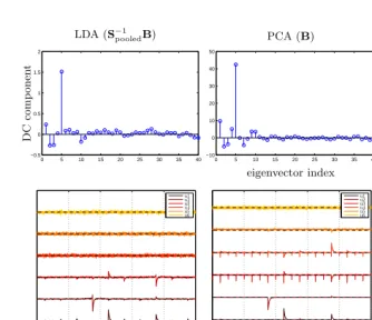
Fig. 8. Top: DC components of eigenvectors of LDA (S−_pooled1 B), PCA (B) andSpooled.

Middle: First six eigenvectors of LDA (S−_pooled1 B), PCA (B) andSpooled. Bottom:

eigen-values (log y axis) of LDA and PCA.

LDA we no longer need a covariance matrix after compression, allows LDA to filter out temperature variations and other noise sources that are similar across campaigns, and provide good results even across different devices.

In order to show how LDA and PCA deal with the DC offset, we show in Figure 8 (top) the DC components (mean) of the LDA and PCA eigenvectors. For LDA we can see that there is a peek at the fifth DC component, which shows that our choice of m = 4 avoided the component with largest DC offset by chance. For PCA we can see a similar peek, also for the fifth component, and again our choice m= 4 avoided this component. However, for PCA this turned out to be bad, because PCA does use a covariance matrix after projection and therefore it would benefit from getting as much knowledge of the temperature variation from the samples. This temperature variation will be given by the eigenvector with a high DC offset and therefore we expect that adding this eigenvector may provide better results. We also show in Figure 8 the first six eigenvectors of LDA (S−_pooled1 B), PCA (B) and Spooled, along with the first 20 eigenvalues of

(16)

100 101 102 103 0

1 2 3 4 5 6

na(log axis)

LDA, m=4 PCA, m=4 sample, 1ppc sample, 3ppc sample, 20ppc sample, allap LDA, m=3 LDA, m=5 LDA, m=6 LDA, m=40 PCA, m=5 PCA, m=6 PCA, m=40

1000 101 102 103 1

2 3 4 5 6

na(log axis)

LDA, m=4 LDA, m=5 PCA, m=4 PCA, m=5

LDAm= 3, m= 4 PCAm= 4

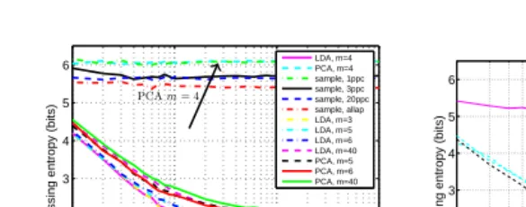
Fig. 9. Template attack on different campaigns (profiling on Alpha, attack on Beta). Left: using various compressions with Method 1. Right: using PCA and LDA with Method 5.

this is not obvious in LDA. Also, we see that the division bySpooledin LDA has

removed much of the noise found in the PCA eigenvectors, and it appears that LDA has reduced the number of components extracting most information from four (in PCA) down to three.

To confirm the above observations, we show in Figure 9 (left) the results of template attacks when using PCA and LDA with different values of m. We see that for LDA there is a great gap between using m = 4 and m = 5, no gap betweenm = 3 andm = 4, while the gap between m= 5 and m= 40 is very small. This confirms our previous observation that with LDA we should ignore the eigenvector containing a strong DC coefficient. Also, we see that for PCA there is a huge gap between usingm= 4 andm= 5 (in the opposite sense as with LDA), but the gap between m = 5 and m = 40 is negligible. Therefore, PCA can work well across devices if we include the eigenvectors containing the DC offset information. These results provide an important lesson for implementing template attacks across different devices or campaigns: the choice of components should consider the DC offset contribution of each eigenvector. This suggests that previous studies may have missed important information, by using only sample selections with one to three samples [12] or only the first PCA component [14].

5.5 Add DC Offset Variation to PCA

Renauld et al. [12] mentioned that“physical variability makes the application of PCA irrelevant, as it cannot distinguish between inter-plaintext and inter-chip

variances”. While it is true that the standard PCA approach [6] is not aimed at

(17)

0 5 10 15 20 25 30 35 40 −35

−30 −25 −20 −15 −10 −5 0 5

0 5 10 15 20 25 30 35 40 −50

−40 −30 −20 −10 0 10

0 500 1000 1500 2000 2500 u1 u2 u3 u4 u5 u6

LDA (S−1

pooledB) PCA (B)

eigenvector index

sample index

DC

com

p

onen

t

Fig. 10. Top: DC components of eigenvectors of LDA (S−_pooled1 B) and PCA (B) after using Method 5. Bottom: First six eigenvectors of LDA (S−_pooled1 B) and PCA (B).

Method 5 (Add Random Offsets to the MatrixB – PCA and LDA only)

1. Obtain the rawleakage traces Xr

k from the profiling device, for each k.

2. Obtain the pooled covariance matrixSpooled∈Rm×m.

3. Pick a random offsetck for each mean vectorx¯k.6

4. Compute the between-groups matrix as

B=P

k∈S(¯x

r

k−x¯

r₊₁r_·_c

k)(¯xrk−x¯

r₊₁r_·_c

k)0.

5. Use PCA (usesB only) or LDA (uses bothB andSpooled) to compress the

rawleakage traces and obtainXk for eachk.

6. Compute the template parameters(¯xk,Spooled)using (1,3).

7. Obtain the compressed leakage tracesXk? from the attacked device.

The results of this method are shown in Figure 9 (right). We see that now PCA provides good results even with m = 4. However, in this case LDA gives bad results withm = 4. In Figure 10 we show the eigenvectors from LDA and PCA, along with their DC component. We can see that, by using this method, we managed to push the eigenvector having the strongest DC component first, and this was useful for PCA. However, LDA does not benefit from including a noise eigenvector into B, so we propose this method only for use with PCA.

6

We have chosen ck uniformly from the interval [−u, u], where u is the absolute

(18)

6 Conclusions

In this paper, we explored the efficacy of template attacks when using different devices for the profiling and attack steps.

We observed that, for our Atmel XMEGA 256 A3U 8-bit microcontroller and particular setup, the campaign-dependent parameters (temperature, envi-ronmental noise, etc.) appear to be the dominant factors in differences between campaign data, not the inter-device variability. These differences rendered the standard template attack useless for all common compression methods except Fisher’s Linear Discriminant Analysis (LDA). To improve the performance of the attack across different devices, we explored several variants of the template attack, that compensate for a DC offset in the attack phase, or profile across multiple devices. By combining these options, we can improve the results of tem-plate attacks. However, these methods did not provide a great advantage when using Principal Component Analysis (PCA) or LDA.

Based on detailed analysis of LDA, we offered an explanation why this com-pression method works well across different devices: LDA is able to compensate temperature variation captured by the pooled covariance matrix and this tem-perature variation is similar across campaigns. From this analysis, we were able to provide guidance for an efficient use of both LDA and PCA across different devices or campaigns: for LDA we should ignore the eigenvectors starting with the one having the strongest DC contribution, while for PCA we should choose enough components to include at least the one with the strongest DC contri-bution. Based on these observations we also proposed a method to enhance the PCA algorithm such that the eigenvector with the strongest DC contribution corresponds to the largest eigenvalue and this allows PCA to provide good re-sults across different devices even when using a small number of eigenvectors.

Our results show that the choice of compression method and parameters (e.g. choice of eigenvectors for PCA and LDA) has a strong impact on the success of template attacks across different devices, a fact that was not evidenced in previous studies. As a guideline, when using sample selection we should use a large number of samples, profile on multiple devices and adapt for a DC offset, but with LDA and PCA we may use the standard template attack and perform the profiling on a single device, if we select the eigenvectors according to their DC component. Overall, LDA seems the best compression method when using template attacks across different devices, but it requires to invert a possibly large covariance matrix, which might not be possible with a small number of profiling traces. In such cases, PCA might be a better alternative.

We conclude that with a careful choice of compression method we can obtain template attacks that are efficient also across different devices, reducing the guessing entropy of an unknown 8-bit value below 1.5 bits.

Data and Code Availability:In the interest of reproducible research we make available our data and related MATLAB scripts at:

(19)

Acknowledgement:Omar Choudary is a recipient of the Google Europe Fellowship in Mobile Security, and this research is supported in part by this Google Fellowship. The opinions expressed in this paper do not represent the views of Google unless otherwise explicitly stated.

References

1. P. Kocher, J. Jaffe, and B. Jun, “Differential Power Analysis”, CRYPTO 1999, LNCS 1666, pp 789–789.

2. S. Chari, J. Rao, and P. Rohatgi, “Template Attacks”, in Cryptographic Hard-ware and Embedded Systems – CHES 2002, LNCS 2523, pp 51–62.

3. E. Brier, C. Clavier, and F. Olivier, “Correlation Power Analysis with a Leakage Model”, in Cryptographic Hardware and Embedded Systems – CHES 2004, LNCS 3156, pp 135–152.

4. W. Schindler, K. Lemke, and C. Paar, “A Stochastic Model for Differential Side Channel Cryptanalysis”, in CHES 2005, LNCS 3659, pp 30–46.

5. B. Gierlichs, K. Lemke-Rust, and C. Paar, “Templates vs. Stochastic Methods”, in CHES 2006, LNCS 4249, 2006, pp 15–29.

6. C. Archambeau, E. Peeters, F. Standaert, and J. Quisquater, “Template Attacks in Principal Subspaces”, in CHES 2006, LNCS 4249, 2006, pp 1–14.

7. N. Homma, S. Nagashima, Y. Imai, T. Aoki, and A. Satoh, “High-Resolution Side-Channel Attack Using Phase-Based Waveform Matching”, in CHES 2006, LNCS 4249, 2006, pp 187–200.

8. F.-X. Standaert and C. Archambeau, “Using Subspace-Based Template Attacks to Compare and Combine Power and Electromagnetic Information Leakages”, in CHES 2008, LNCS 5154, pp 411–425.

9. B. Gierlichs, L. Batina, P. Tuyls, and B. Preneel, “Mutual Information Analy-sis”, in CHES 2008, LNCS 5154, pp 426–442.

10. F.-X. Standaert, T. G. Malkin, and M. Yung, “A Unified Framework for the Analysis of Side-Channel Key Recovery Attacks”, in Proceedings of the 28th Annual International Conference on Advances in Cryptology: the Theory and Applications of Cryptographic Techniques, Berlin, Heidelberg, 2009, pp 443– 461.

11. F.-X. Standaert, F. Koeune, and W. Schindler, “How to Compare Profiled Side-Channel Attacks?” in Applied Cryptography and Network Security, LNCS 5536, pp 485–498.

12. M. Renauld, F.-X. Standaert, N. Veyrat-Charvillon, D. Kamel, and D. Flan-dre, “A Formal Study of Power Variability Issues and Side-Channel Attacks for Nanoscale Devices”, in EUROCRYPT 2011, LNCS 6632, pp 109–128.

13. D. Oswald and C. Paar, “Breaking Mifare DESFire MF3ICD40: Power Analysis and Templates in the Real World”, in CHES 2011, LNCS 6917, pp 207–222. 14. M. A. Elaabid and S. Guilley, “Portability of templates”, Journal of

Crypto-graphic Engineering, 2(1), pp 63–74, 2012.

15. A. Heuser, M. Kasper, W. Schindler, and M. St¨ottinger, “A New Difference Method for Side-Channel Analysis with High-Dimensional Leakage Models”, in CT-RSA 2012, LNCS 7178, pp. 365–382.

16. V. Lomn´e, E. Prouff, and T. Roche, “Behind the Scene of Side Channel Attacks”, in Advances in Cryptology - ASIACRYPT 2013, pp. 506–525.