How to Fake Auxiliary Input
Dimitar Jetchev and Krzysztof Pietrzak⋆
EPFL Switzerland and IST Austria
Abstract. Consider a joint distribution (X, A) on a setX × {0,1}ℓ. We show that for any family
F of distinguishersf:X × {0,1}ℓ→ {0,1}, there exists a simulatorh:X → {0,1}ℓsuch that
1. no function inF can distinguish (X, A) from (X, h(X)) with advantageǫ, 2. his onlyO(23ℓǫ−2) times less efficient than the functions inF.
For the most interesting settings of the parameters (in particular, the cryptographic case whereX has superlogarithmic min-entropy,ǫ >0 is negligible andF consists of circuits of polynomial size), we can make the simulatorhdeterministic.
As an illustrative application of this theorem, we give a new security proof for the leakage-resilient stream-cipher from Eurocrypt’09. Our proof is simpler and quantitatively much better than the original proof using the dense model theorem, giving meaningful security guarantees if instantiated with a standard blockcipher like AES.
Subsequent to this work, Chung, Lui and Pass gave an interactive variant of our main theorem, and used it to investigate weak notions of Zero-Knowledge. Vadhan and Zheng give a more constructive version of our theorem using their new uniform min-max theorem.
1
Introduction
Let X be a set and let ℓ > 0 be an integer. We show that for any joint distribution (X, A) over X × {0,1}ℓ (where we think of A as a short ℓ-bit auxiliary input to X), any
family F of functions X × {0,1}ℓ → {0,1} (thought of as distinguishers) and anyε >0,
there exists an efficient simulator h: X → {0,1}ℓ for the auxiliary input that fools every
distinguisher in F, i.e.,
∀f ∈ F: |E[f(X, A)]−E[f(X, h(X))]|< ε.
Here, “efficient” means that the simulator h is ˜O(23ℓε−2) times more complex than the
functions fromF (we will formally define “more complex” in Definition 6). Without loss of generality, we can model the joint distribution (X, A) as (X, g(X)), where g is some arbi-trarily complex and possibly probabilistic function (whereP[g(x) =a] =P[A =a|X =x]
for all (x, a)∈ X × {0,1}ℓ). Let us stress that, as g can be arbitrarily complex, one
can-not hope to get an efficient simulator h where (X, g(X)) and (X, h(X)) are statistically close. Yet, one can still fool all functions in F in the sense that no function from F can distinguish the distribution (X, A) from (X, g(X)).
Relation to [25]. Trevisan, Tulsiani and Vadhan [25, Thm. 3.1] prove a conceptually
similar result, stating that if Z is a set then for any distribution Z over Z, any family e
F of functions Z → [0,1] and any function eg: Z → [0,1], there exists a simulator e
h: Z → [0,1] whose complexity is only O(ε−2) times larger than the complexity of the
functions from Fe such that
∀fe∈Fe : |E[fe(Z)eg(Z)]−E[fe(Z)eh(Z)]|< ε. (1)
⋆ Supported by the European Research Council under the European Union’s Seventh Framework Programme
In [25], this result is used to prove that every high-entropy distribution is indistinguishable from an efficiently samplable distribution of the same entropy. Moreover, it is shown that many fundamental results including the Dense Model Theorem [23,14,21,10,24], Impagliazzo’s hardcore lemma [18] and a version of Sz´emeredi’s Regularity Lemma [11] follow from this theorem. The main difference between (1) and our statement
∀f ∈ F: |E[f(X, g(X))]−E[f(X, h(X))]|< ε (2)
is that our distinguisher f sees not onlyX, but also the real or fake auxiliary inputg(X) or h(X), whereas in (1), the distinguisher feonly sees X. In particular, the notion of indistinguishability we achieve captures indistinguishability in the standard cryptographic sense. On the other hand, (1) is more general in the sense that the range of f ,eeg,eh can be any real number in [0,1], whereas our f has range {0,1} and g, h have range {0,1}ℓ.
Nonetheless, it is easy to derive (1) from (2): consider the case ofℓ= 1 bit of auxiliary input, and only allow families F of distinguishers where each f ∈ F is of the form
f(X, b) = fb(X)b for some function fb: X → [0,1]. For this restricted class, the absolute value in (2) becomes
|E[f(X, g(X))]−E[f(X, h(X))|=|E[fb(X)g(X)]−E[fb(X)h(X)]| (3)
Asfbis arbitrary, this restricted class almost captures the distinguishers considered in (1). The only difference is that the functioneg has range [0,1] whereas our g has range {0,1}. Yet, note that in (1), we can replace eg having range [0,1] by a (probabilistic) g with range {0,1}defined as P[g(x) = 1] =ge(x), thus, leaving the expectation E[fe(X)eg(X)] = E[fe(X)g(X)] unchanged.1
In [25], two different proofs for (1) are given. The first proof uses duality of linear programming in the form of the min-max theorem for two-player zero-sum games. This proof yields a simulator of complexityO(ε−4log2(1/ε)) times the complexity of the
func-tions inF. The second elegant proof uses boosting and gives a quantitatively much better
O(ε−2) complexity.
Proof outline. As it was just explained, (1) follows from (2). We do not know if one
can directly prove an implication in the other direction, so we prove (2) from scratch. Similarly to [25], the core of our proof uses boosting with the same energy function as the one used in [25].
As a first step, we transform the statement (2) into a “product form” like (1) where
Z =X × {0,1}ℓ (this results in a loss of a factor of 2ℓ in the advantage ε; in addition,
our distinguishers fb will have range [−1,1] instead of [0,1]). We then prove that (1) holds for some simulatoreh: Z →[0,1] of complexityε−2 relative toF. Unfortunately, we
cannot use the result from [25] in a black-box way at this point as we need the simulator e
h: Z →[0,1] to define a probability distribution in the sense thateh(x, b)≥0 for all (x, b)
and X
b∈{0,1}ℓ
eh(x, b) = 1 for allx. Ensuring these conditions is the most delicate part of the
1 The simulatorehfrom [25] satisfies the additional property|E[eh(X)]−E[
e
proof. Finally, we show that the simulator h defined via P[h(x) = b] = eh(x, b) satisfies
(2). Note that for hto be well defined, we needeh to specify a probability distribution as outlined above.
Efficiency of h. Our simulator h is efficient in the sense that it is only O(23ℓε−2) times
more complex than the functions inF. We do not know how tight this bounds is, but one can prove a lower bound of max{2ℓ, ε−1} under plausible assumptions. The dependency
on 2ℓ is necessary under exponential hardness assumptions for one-way functions.2 A
dependency onε−1 is also necessary. Indeed, Trevisan et al. [25, Rem. 1.6] show that such
a dependency is necessary for the simulator eh in (1). Since (1) is implied by (2) with h
and eh having exactly the same complexity, the ε−1 lower bound also applies to our h.
1.1 Subsequent work
The original motivation for this work was to give simpler and quantitatively better proofs for leakage-resilient cryptosystems as we will discuss in Section 4. Our main theorem has subsequently been derived via two different routes.
First, Chung, Lui and Pass [4] investigate weak notions of zero-knowledge. On route, they derive an “interactive” version of our main theorem. In Section 4, we will show how to establish one of their results (with better quantitative bounds), showing that every interactive proof system satisfies a weak notion of zero-knowledge.
Second, Vadhan and Zheng [26, Thm.3.1-3.2] recently proved a version of von Neu-mann’s min-max theorem for two-player zero sum games that does not only guarantee existence of an optimal strategy for the second player, but also constructs a nearly optimal strategy assuming knowledge of several best responses of the second player to strategies of the first player, and provide many applications of this theorem. Their argument is based on relative entropy KL projections and a learning technique known as weight updates and resembles the the proof of the Uniform Hardcore Lemma by Barak, Hardt and Kale [2] (see also [16] for the original application of this method). They derive our main theorem [26, Thm.6.8], but with incomparable bounds. Concretely, to fool circuits of size t, their simulator runs in time ˜O(t·2ℓ/ε2+2ℓ/ε4) compared to ours whose run-time is ˜O(t·23ℓ/ε2).
In particular, their bounds are better whenever 1/ε2 ≤t·22ℓ. The additive 2ℓ/ε4 term in
their running time appears due to the sophisticated iterative“weight update” procedure, whereas our simulator simply consists of a weighted sum of the evaluation of ˜O(23ℓ/ε2)
circuits from the family we want to fool (here, circuits of size t).
1.2 More applications
Apart from reproving one of [4]’s results on weak zero-knowledge mentioned above, we give two more applications of our main theorem in Section 4:
Chain Rules for Computational Entropy. In a recent paper, Gentry and Wichs [13]
show that black-box reductions cannot be used to prove the security of any succinct non-interactive argument from any falsifiable cryptographic assumption. A key techni-cal lemma used in their proof ([13, Lem. 3.1]) states that if two distributions X and Xe
2 More precisely, assume there exists a one-way function where inverting becomes 2ℓtimes easier givenℓbits of
over X are computationally indistinguishable, then for any joint distribution (X, A) over
X ×{0,1}ℓ (here,Ais a shortℓ-bit auxiliary input) there exists a joint distribution (X,e Ae)
such that (X, A) and (X,e Ae) are computationally indistinguishable. Our theorem imme-diately implies the stronger statement that not only such an (X,e Ae) exists, but in fact, it is efficiently samplable, i.e., there exists an efficient simulator h: X → {0,1}ℓ such that
(X, he (Xe)) is indistinguishable from (X,e Ae) and thus from (X, A). Reyzin [22, Thm.2] ob-served that the result of Gentry and Wichs implies a chain rule for conditional “relaxed” HILL entropy. We give a short and simple proof of this chain rule in Proposition 2 of this paper. We then show in Corollary 1 how to deduce a chain rule for (regular) HILL entropy from Proposition 2 using the simple fact (Lemma 1) that short (i.e., logarithmic in the size of the distinguishers) computationally indistinguishable random variables must al-ready be statistically close. Chain rules for HILL entropy have found several applications in cryptography [10,21,7,12]. The chain rule that we get in Corollary 1 is the first one that does not suffer from a significant loss in the distinguishing advantage (we only lose a constant factor of 4). Unlike the case of relaxed HILL-entropy, here we only prove a chain rule for the ”non-conditional” case, which is a necessary restriction given a recent counterexample to the (conditional) HILL chain rule by Krenn et al. [19]. We will provide more details on this negative result after the statement of Corallary 1.
Leakage Resilient Cryptography. The original motivation for this work is to simplify the security proofs of leakage-resilient [10,20,7] and other cryptosystems [12] whose security proofs rely on chain rules for computational entropy (as discussed in the previous para-graph). The main idea is to replace the chain rules with simulation-based arguments. In a nutshell, instead of arguing that a variable X must have high (pseudo)entropy in the presence of a short leakage A, one could simply use the fact that the leakage can be efficiently simulated. This not only implies that X has high (pseudo)entropy given the fake leakage h(X), but if X is pseudorandom, it also implies that (X, h(X)) is indistin-guishable from (U, h(U)) for a uniform random variable U on the same set asX. In the security proofs, we would now replace (X, h(X)) with (U, h(U)) and will continue with a uniformly random intermediate variable U. In contrast, the approach based on chain rules only tells us that we can replace X with some random variable Y that has high min-entropy given A. This is not only much complex to work with, but it often gives weaker quantitative bounds. In particular, in Section 4.3 we revisit the security proof of the leakage-resilient stream-cipher from [20] for which we can now give a conceptually simpler and quantitatively better security proof.
2
Notation and Basic Definitions
2.1 Notation
We use calligraphic letters such as X to denote sets, the corresponding capital letters
X to denote random variables on these sets (equivalently, probability distributions) and lower-case letters (e.g., x) for values of the corresponding random variables. Moreover,
x ← X means that x is sampled according to the distribution X and x ← X means that xis sampled uniformly at random fromX. LetUn denote the random variable with
uniform distribution on {0,1}n. We denote by ∆(X;Y) = 1
2 X
x∈X
the statistical distance between X andY. Forε >0, s ∈N, we use X ∼Y to denote that
X and Y have the same distribution, X ∼εY to denote that their statistical distance is
less thanεandX ∼ε,s Y to denote that no cicurit of sizescan distinguishX fromY with
advantage greater thanε. Note thatX ∼ε,∞Y ⇐⇒ X ∼εY andX ∼0 Y ⇐⇒ X ∼Y.
probabilistic (randomized) function then we will use [h] to denote the random coins used byh (a notation that will be used in various probabilities and expectations).
2.2 Entropy Measures
A random variableX has min-entropy k, if no (even computationally unbounded) adver-sary can predict the outcome of X with probability greater than 2−k.
Definition 1. (Min-Entropy H∞) A random variable X has min-entropy k, denoted H∞(X)≥k, if max
x P[X =x]≤2
−k.
Dodis et al. [8] gave a notion of average-case min-entropy defined such thatXhas average-case min-entropyk conditioned onZ if the probability of the best adversary in predicting
X given Z is 2−k.
Definition 2. (Average min-Entropy [8] He∞) Consider a joint distribution (X, Z),
then the average min-entropy of X conditioned on Z is
e
H∞(X|Z) =−log
E z←Z
h max
x P[X =x|Z =z]
i
=−log
E z←Z
2−H∞(X|Z=z)
HILL-entropy is the computational analogue of min-entropy. A random variable X has HILL-entropyk if there exists a random variableY having min-entropyk that is indistin-guishable from X. HILL-entropy is further quantified by two parameters ε, s specifying this indistinguishability quantitatively.
Definition 3. (HILL-Entropy [15]HHILL
)X has HILL entropyk, denoted byHHILL
ε,s (X)≥
k, if
HHILL
ε,s (X)≥k ⇐⇒ ∃Y : H∞(Y)≥k and X ∼ε,s Y
Conditional HILL-entropy has been defined by Hsiao, Lu and Reyzin [17] as follows.
Definition 4. (Conditional HILL-Entropy [17]) X has conditional HILL entropy k
(conditioned on Z), denoted HHILL
ε,s (X|Z)≥k, if
HHILL
ε,s (X|Z)≥k ⇐⇒ ∃(Y, Z) : He∞(Y|Z)≥k and (X, Z)∼ε,s (Y, Z)
Note that in the definition above, the marginal distribution on the conditional part Z
is the same in both the real distribution (X, Z) and the indistinguishable distribution (Y, Z). A “relaxed” notion of conditional HILL used implicitly in [13] and made explicit in [22] drops this requirement.
Definition 5. (Relaxed Conditional HILL-Entropy [13,22]) X has relaxed
condi-tional HILL entropy k, denoted Hrlx-HILL
ε,s (X|Z)≥k, if
Hrlx-HILL
3
The main theorem
Definition 6. (Complexity of a function) Let A and B be sets and let G be a family
of functions h: A → B. A function h has complexity C relative to G if it can be
computed by an oracle-aided circuit of sizepoly(Clog|A|)withC oracle gates where each oracle gate is instantiated with a function from G.
Theorem 1. (Main) Let ℓ ∈ N be fixed, let ε > 0 and let X be any set. Consider a
distribution X over X and any (possibly probabilistic and not necessarily efficient) func-tion g: X → {0,1}ℓ. Let F be a family of deterministic (cf. remark below) distinguishers
f: X × {0,1}ℓ → {0,1}. There exists a (probabilistic) simulator h : X → {0,1}ℓ with
complexity3
O(23ℓε−2log2(ε−1))
relative to F that ε-fools every distinguisher in F, i.e.
∀f ∈ F :
x←EX,[g][f(x, g(x))]−x←EX,[h][f(x, h(x))]
< ε, (4)
Moreover, if
H∞(X)>2 + log log|F|+ 2 log(1/ε) (5)
then there exists a deterministic h with this property.
Remark 1 (Closed and ProbabilisticF).In the proof of Theorem 1 we assume that the
class F of distinguishers is closed under complement, i.e., if f ∈ F then also 1−f ∈ F. This is without loss of generality, as even if we are interested in the advantage of a class F that is not closed, we can simply apply the theorem for F′ = F ∪ (1− F), where (1− F) = {1−f : f ∈ F}. Note that if h has complexity t relative to F′, it has the same complexity relative to F. We also assume that all functions f ∈ F are deterministic. If we are interested in a class F of randomized functions, we can simply apply the theorem for the larger class of deterministic functionsF′′consisting of all pairs (f, r) where f ∈ F and r is a choice of randomness for f. This is almost without loss of generality, except that the requirement in (5) on the min-entropy of X becomes slightly stronger as log log|F′′| = log log(|F|2ρ) where ρ is an upper bound on the number of
random coins used by any f ∈ F.
4
Applications
4.1 Zero-Knowledge
Chung, Lui and Pass [4] consider the following relaxed notion of zero-knowledge
Definition 7 (distributional (T, t, ε)-zero-knowledge). Let (P,V) be an interactive proof system for a languageL. We say that(P,V)is distributional (T, t, ε)-zero-knowledge
(whereT, t, εare all functions ofn) if for everyn ∈N, every joint distributions(Xn, Yn, Zn)
3 If we modelhas a Turing machine (and not a circuit) and consider the expected complexity ofh, then we
over (L∩ {0,1}n)× {0,1}∗× {0,1}∗, and every t-size adversaryV∗, there exists a T-size
simulator S such that
(Xn, Zn,outV∗[P(Xn, Yn)↔ V∗(Xn, Zn)])∼ε,t (Xn, Zn, S(Xn, Zn))
where outV∗[P(Xn, Yn)↔ V∗(Xn, Zn)] denotes the output of V∗(Xn, Zn) after interacting
with P(Xn, Yn).
IfLin an NP language, then in the definition above,Y would be a witness forX ∈L. As a corollary of their main theorem, [4] show that every proof system satisfies this relaxed notion of zero-knowledge where the running time T of the simulator is polynomial in t, ε
and 2ℓ. We can derive their Corollary from Theorem 1 with better quantitative bounds
for most ranges of parameteres than [4]: we get ˜O(t23ℓε−2) vs. ˜O(t32ℓε−6), which is better
whenever t/ε2 ≥2ℓ.
Proposition 1. Let (P,V) be an interactive proof system for a languageL, and suppose that the total length of the messages sent by P isℓ=ℓ(n)(on common inputs X of length
n). Then for any t = t(n) ≥ Ω(n) and ε = ε(n), (P,V) is distributional (T, t, ε) -zero-knowledge, where
T =O(t23ℓε−2log2(ε−1))
Proof. LetM ∈ {0,1}ℓdenote the messages send byP(X
n, Yn) when talking toV∗(Xn, Zn).
By Theorem 1 (identifyingF from the theorem with circuits of size t) there exists a sim-ulator h of size O(t·23ℓε−2log2(ε−1)) s.t.
(Xn, Zn, M)∼ε,2t(Xn, Zn, h(Xn, Zn)) (6)
Let S(Xn, Zn) be defined as follows, first compute M′ = h(Xn, Zn) (with h as above),
and then compute out∗
V[M′ ↔ V∗(Xn, Zn)]. We claim that
(Xn, Zn,outV∗[P(Xn, Yn)↔ V∗(Xn, Zn)])∼ε,t (Xn, Zn, S(Xn, Zn)) (7)
To see this, note that from any distinguisherDof sizetthat distinguishes the distributions in (7) with advantage δ > ε, we get a distinguisher D′ of size 2t that distinguishes the distributions in (6) with the same advantage by defining D′ as D′(Xn, Zn,M˜) = D(Xn, Zn,outV∗[ ˜M ↔ V∗(Xn, Zn)]). ⊓⊔
4.2 Chain Rules for (Conditional) Pseudoentropy
The following proposition is a chain rule for relaxed conditional HILL entropy. Such a chain rule for the non-conditional case is implicit in the work of Gentry and Wichs [13], and made explicit and generalized to the conditional case by Reyzin [22].
Proposition 2. ([13,22]) Any joint distribution(X, Y, A)∈ X × Y × {0,1}ℓ satisfies4
Hrlx-HILL
ε,s (X|Y)≥k ⇒ H
rlx-HILL
2ε,ˆs (X|Y, A)≥k−ℓ where ˆs=Ω
s· ε
2
23ℓlog2(1/ε)
4 Using the recent bound from [26] discussed in Section 1.1, we can get ˆs=Ωs·ε2ℓ
2ℓ +
ℓ2log2(1/ε)
ε4
Proof. Recall that Hrlx-HILL
ε,s (X|Y)≥ k means that there exists a random variable (Z, W)
such thatH∞(Z|W)≥kand (X, Y)∼ε,s (Z, W). For any ˆε,ˆs, by Theorem 1, there exists a simulator hof sizesh =O
ˆ
s· 23ℓlogεˆ22(1/εˆ)
such that (we explain the second step below)
(X, Y, A)∼ε,ˆsˆ(X, Y, h(X, Y))∼ε,s−sh (Z, W, h(Z, W))
The second step follows from (X, Y)∼ε,s (Z, W) and the fact thath has complexity sh.
Using the triangle inequality for computational indistinguishability5 we get
(X, Y, A)∼εˆ+ε,min(ˆs,s−sh) (Z, W, h(Z, W))
To simplify this expression, we set ˆε:=ε and ˆs:=Θ(sε2/23ℓlog2(1/ε)), then s
h =O(s),
and choosing the hidden constant in theΘsuch thatsh ≤s/2 (and thus ˆs ≤s−sh =s/2),
the above equation becomes
(X, Y, A)∼2ε,sˆ(Z, W, h(Z, W)) (8)
Using the chain rule for average case min-entropy in the first, and H∞(Z|W)≥k in the second step below we get
e
H∞(Z|W, h(Z, W))≥He∞(Z|W)−H0(h(Z, W))≥k−ℓ . (9)
Now equations (8) and (9) imply Hrlx-HILL
2ε,ˆs (X|Y, A) = k−ℓ as claimed. ⊓⊔
By the following lemma, conditional relaxed HILL implies conditional HILL if the con-ditional part is short (at most logarithmic in the size of the distinguishers considered.)
Lemma 1. For a joint random variable (X, A) over X × {0,1}ℓ and s = Ω(ℓ2ℓ) (more
concretely, s should be large enough to implement a lookup table for a function {0,1}ℓ → {0,1}) conditional relaxed HILL implies standard HILL entropy
Hrlx-HILL
ε,s (X|A)≥k ⇒ H
HILL
2ε,s (X|A)≥k
Proof. Hrlx-HILL
ε,s (X|A)≥k means that there exist (Z, W) where He∞(Z|W)≥k and
(X, A)∼ε,s (Z, W) (10)
We claim that if s = Ω(ℓ2ℓ), then (10) implies that W ∼
ε A. To see this, assume
the contrary, i.e., that W and A are not ε-close. There exists then a computationally unbounded distinguisher D where
|P[D(W) = 1]−P[D(A) = 1]|> ε.
Without loss of generality, we can assume that D is deterministic and thus, implement
D by a circuit of size Θ(ℓ2ℓ) via a lookup table with 2ℓ entries (where the ith entry is
5 which states that for any random variablesα, β, γwe have
D(i).) Clearly, D can also distinguish (X, A) from (Z, W) with advantage greater thanε
by simply ignoring the first part of the input, thus, contradicting (10). As A ∼ε W, we
claim that there exist a distribution (Z, A) such that
(Z, W)∼ε(Z, A). (11)
This distribution (Z, A) can be sampled by first sampling (Z, W) and then outputting (Z, α(W)) where α is a function that is the identity with probability at least 1−ε (over the choice of W), i.e., α(w) =w and with probability at most ε, it changes W so that it matches A. The latter is possible since A ∼ε W.
Using the triangle inequality for computational indistinguishability (cf. the proof of Proposition 2) we get with (10) and (11)
(X, A)∼2ε,s (Z, A) (12)
As He∞(Z|W)≥k (for α as defined above)
e
H∞(Z|W)≥k ⇒ He∞(Z|α(W))≥k ⇒ He∞(Z|A)≥k (13)
The first implication above holds as applying a function on the conditioned part cannot decrease the min-entropy. The second holds as (Z, A) ∼ (Z, α(W)). This concludes the proof as (12) and (13) imply that HHILL
2ε,s(X|A)≥k. ⊓⊔
As a corollary of Proposition 1 and Lemma 1, we get a chain rule for (non-conditional) HILL entropy. Such a chain rule has been shown by [10] and follows from the more general Dense Model Theorem (published at the same conference) of Reingold et al. [21].
Corollary 1. For any joint distribution (X, A)∈ X × {0,1}ℓ and ˆs=Ω s·ε2
23ℓlog2(ℓ)
HHILL
ε,s (X)≥k ⇒H
rlx-HILL
2ε,ˆs (X|A)≥k−ℓ ⇒H
HILL
4ε,sˆ(X|A)≥k−ℓ
Note that unlike the chain rule for relaxed HILL given in Proposition 2, the chain rule for (standard) HILL given by the corollary above requires that we start with some non-conditional variable X. It would be preferable to have a chain rule for the conditional case, i.e., and expression of the form HHILL
ε,s (X|Y) =k ⇒H
HILL
ε′,s′(X|Y, A) = k−ℓ for some
ε′ =ε·p(2ℓ), s′ =s/q(2ℓ, ε−1) (for polynomial functions p(.), q(.)), but as recently shown
by Krenn et al. [19], such a chain rule does not hold (all we know is that such a rule holds if we also allow the security to degrade exponentially in the length |Y| of the conditional part.)
4.3 Leakage-Resilient Cryptography
For brevity, in this section we often write Bi to denote a sequence B
1, . . . , Bi of
values. Moreover, AkB ∈ {0,1}a+b denotes the concatenation of the strings A ∈ {0,1}a
and B ∈ {0,1}b.
A function F: {0,1}k × {0,1}n → {0,1}m is an (ε, s, q)-secure weak PRF if its
outputs onq random inputs look random to any sizes distinguisher, i.e., for allDof size
s
K,XPq[
D(Xq,F(K, X1), . . . ,F(K, Xq) = 1]− P Xq,Rq[
D(Xq, Rq) = 1 ≤ε,
where the probability is over the choice of the random Xi ← {0,1}n, the choice of a
random key K ← {0,1}k and random Ri ← {0,1}m conditioned on Ri =Rj if Xi =Xj
for some j < i.
A stream-cipher SC:{0,1}k → {0,1}k× {0,1}nis a function that, when initialized
with a secret initial state S0 ∈ {0,1}k, produces a sequence of output blocks X1, X2, . . .
recursively computed by
(Si, Xi) := SC(Si−1)
We say that SC is (ε, s, q)-secure if for all 1 ≤ i ≤ q, no distinguisher of size s can distinguish Xi from a uniformly random Un ← {0,1}n with advantage greater than ε
givenX1, . . . , Xi−1 (here, the probability is over the choice of the initial random keyS0)6,
i.e.,
SP0
[D(Xi−1, Xi) = 1]− P
S0,Un
[D(Xi−1, Un] ≤ε
A leakage-resilient stream-cipher is (ε, s, q, ℓ)-secure if it is (ε, s, q)-secure as just defined, but where the distinguisher in the jth round not only gets Xj, but also ℓ bits
of arbitrary adaptively chosen leakage about the secret state accessed during this round. More precisely, before (Sj, Xj) :=SC(Sj−1) is computed, the distinguisher can choose any
leakage function fj with range{0,1}ℓ, and then not only getXj, but alsoΛj :=fj( ˆSj−1),
where ˆSj−1 denotes the part of the secret state that was modified (i.e., read and/or
overwritten) in the computation SC(Sj−1).
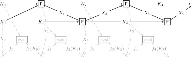
Figure 1 illustrates the construction of a leakage-resilient stream cipher SCF from any weak PRF F: {0,1}k × {0,1}n → {0,1}k+n from [20]. The initial state is S0 =
{K0, K1, X0}. Moreover, in theith round (starting with round 0), one computesKi+2kXi+1 :=
F(Ki, Xi) and outputs Xi+1. The state after this round is (Ki+1, Ki+2, Xi+1).7 In this sec-tion we will sketch a proof of the following security bound on SCF as a leakage-resilient stream cipher in terms of the security ofF as a weak PRF.
Lemma 2. If F is a(εF, sF,2)-secure weak PRF then SCF is a (ε′, s′, q, ℓ)-secure leakage
resilient stream cipher where
ε′ = 4qpεF2ℓ s′ =Θ(1)
· sFε
′2
23ℓ
6 A more standard notion would requireX
1, . . . , Xq to be indistinguishable from random; this notion is implied
by the notion we use by a standard hybrid argument losing a multiplicative factor ofqin the distinguishing advantage.
7 Note thatX
i is not explicitly given as input tofi even though the computation depends on Xi. The reason
The bound above is quantitatively much better than the one in [20]. Setting the leakage bound ℓ = logε−F1/6 as in [20], we get (for small q) ε′ ≈ε
5/12
F , which is by over a power of 5 better than the ε1F/13 from [20], and the bound ons′ ≈sFε4F/3 improves by a factor of
ε5F/6 (fromsFε
13/6
F in [20] tosFε
8/6
F here). This improvement makes the bound meaningful if instantiated with a standard block-cipher like AES which has a keyspace of 256 bits, making the assumption that it provides sF/εF ≈2256 security.8
Besides our main Theorem 1, we need another technical result which states that if F is a weak PRF secure against two queries, then its output on a single random query is pseudorandom, even if one is given some short auxiliary information about the uniform key K. The security of weak PRFs with non-uniform keys has first been proven in [20], but we will use a more recent and elegant bound from [1]. As a corollary of [1, Thm.3.7 in eprint version], we get that for any (εF, sF,2)-secure weak PRFF: {0,1}k× {0,1}n→
{0,1}m, uniform and independent key and input K ∼ U
k, X ∼ Un and any (arbitrarily
complex) function g:{0,1}k→ {0,1}ℓ, one has9
(X,F(K, X), g(K))∼ε,sˆ
F/2 (X, Um, g(K)) where ˆε=εF+
p
εF2ℓ+ 2−n
≈pεF2ℓ (14)
Generalizing the notation of ∼ε,s from variables to interactive distinguishers, given two
(potentially stateful) oracles G, G′, we write G ∼
ε,s G′ to denote that no oracle-aided
adversary Aof size s can distinguish Gfrom G′, i.e.,
G∼ε,s G′ ⇐⇒ ∀A,|A| ≤s : |P[AG →1]−P[AG ′
→1]| ≤ε.
Proof (of Lemma 2 (Sketch)). We define an oracleGreal
0 that models the standard attack
on the leakage-resilient stream cipher. That is, Greal
0 samples a random initial state S0.
When interacting with an adversary AGreal0 , the oracle Greal
0 expects as input adaptively
chosen leakage functions f1, f2, . . . , fq−1. On input fi, it computes the next output block
(Xi, Ki+1) :=SC(Ki−1, Xi−1) and the leakageΛi =fi(Ki−1). It forwards Xi, Λi to A and
deletes everything except the stateSi ={Xi, Ki, Ki+1}. After roundq−1,Greal0 computes
and forwards Xq (i.e., the next output block to be computed) to A. The game Grand0 is
defined in the same way, but the final block Xq is replaced with a uniformly random Un.
To prove that SCF is an (ε′, s′, ℓ, q)-secure leakage-resilient stream cipher, we need to show that
Greal0 ∼ε′,s′ Grand0 , (15)
for ε′, s′ as in the statement of the lemma.
Defining gamesGreal
i andGrandi for1≤i≤q−1. We define a series of gamesGreal1 , . . . , Grealq−1
where Greal
i+1 is derived from Greali by replacing Xi, Ki+1 with uniformly random values
˜
Xi,K˜i+1 and the leakage Λi with simulated fake leakage ˜Λi (the details are provided
below). Games Grand
i will be defined exactly as Greali except that (similarly to the case
i= 0), the last block Xq is replaced with a uniformly random value.
8 We just need security against two random queries, so the well known non-uniform upper bounds on the security
of block-ciphers of De, Trevisan and Tulsiani [6,5] do not seem to contradict such an assumption even in the non-uniform setting.
9 The theorem implies a stronger statement where one only requires thatK hask−ℓbits average-case
For every i, 1≤i≤q−1, the variables ˜Ki,X˜i as defined by the oracles realizing the
gamesGrand
j andGrealj wherej ≥iwill satisfy the following properties (as the initial values
(X0, K0, K1) never get replaced, for notational convenience we define ( ˜X0,K˜0,K˜1)
def = (X0, K0, K1))
i. ˜Ki,X˜i are uniformly random.
ii. Right before the (i−1)th round (i.e. the round where the oracle computesXikKi+1 :=
F( ˜Xi−1,K˜i−1)), the oracle has leaked no information about ˜Ki−1 except for the ℓ bits fake leakage ˜Λi.
iii. Right before the (i−1)th round ˜Ki−1 and ˜Xi−1 are independent given everything the
oracle did output so far.
The first two properties above will follow from the definition of the games. The third point follows using Lemma 4 from [9], we will not discuss this here in detail, but only men-tion that the reason for the alternating structure of the cipher as illustrated in Figure 1, with an upper layer computing K0, K2, . . .and the lower layer computing K1, K3, . . ., is
to achieve this independence.
We now describe how the oracle Greal
i+1 is derived from Greali . For concreteness, we set
i= 2. In the third step,Greal
2 computes (X3, K4) :=F( ˜K2,X˜2), Λ3 =f3( ˜K2) and forwards
X3, Λ3 to A. The state stored after this step isS3 ={X3,K˜3, K4}. Let V2
def
= {X˜2,Λ˜2} be
the view (i.e. all the outputs she got from her oracle) of the adversaryAafter the second round.
Defining an intermediate oracle. We now define an oracleGreal
2/3 (which will be in-between
Greal
2 and Greal3 ) derived from Greal2 by replacing Λ3 =f3( ˜K2) with fake leakage ˜Λ3
com-puted as follows: let h(·) be a simulator for the leakage ˜Λ3 :=f3( ˜K2) such that (for ˆε,ˆs
to be defined)
(Z, h(Z))∼ε,ˆsˆ(Z,Λ˜3) where Z ={V2, X3, K4} (16)
By Theorem 1, there exists such a simulator of size sh
def
= O(ˆs23ℓ/εˆ2). Note that h not
only gets the pseudorandom output X3, K4 whose computation has leaked bits, but also
the view V2. The reason for the latter is that we need to fool an adversary who learned
V2. Equation (16) then yields
Greal2 ∼ε,ˆˆs−s0 G
real
2/3, (17)
where s0 is the size of a circuit required to implement the real game Greal0 . The reason
we loose s0 in the circuit size here is that in a reduction where we use a distinguisher for
Greal
2 and Greal2/3 to distinguish (Z, h(Z)) and (Z,Λ˜3) we must still compute the remaining
q−4 rounds, and s0 is an upper bound on the size of this computation.
The game Greal3 is derived from Greal2/3 by replacing the values X3kK4 := F( ˜K2,X˜2)
with uniformly random ˜X3kK˜4 right after they have been computed (let us stress that
also the fake leakage that is computed as in (16) now uses these random values, i.e.,
Z ={V2,X˜3,K˜4}).
Proving indistinguishability. We claim that the games are indistinguishable with param-eters
Greal2/3 ∼√
εF2ℓ,sF/2−sh−s0 G
real
Recall that in Greal
2/3, we compute X3kK4 :=F( ˜K2,X˜2) where by i. ˜X2,K˜2 are uniformly
random, by ii. only ℓ bits of ˜K2 have leaked and iii. ˜X2 and ˜K2 are independent.
Us-ing these properties, equation (14) implies that the outputs are roughly (√εF2ℓ, sF/2) pseudorandom, i.e.,
( ˜X2, X3kK4,Λ˜1)∼√ε
F2ℓ,sF/2 ( ˜X2,
˜
X3kK˜4,Λ˜1), (19)
from which we derive (18). Note the loss of sh in circuit size in equation (18) due to the
fact that given a distinguisher for Greal
2/3 and Greal3 , we must recompute the fake leakage
given only distributions as in (19).
We will assume that s0 ≤s/ˆ 2, i.e., the real experiment is at most half as complex as
the size of the adversaries we will consider (the setting where this is not the case is not very interesting anyway.) Then ˆs−s0 ≥s/ˆ 2.
Up to this point, we have not yet defined what ˆε and ˆs are, so we set them to
ˆ
εdef= pεF2ℓ and sˆdef= Θ(1)sFεˆ
2
23ℓ then sF = 8·sh =Θ(1)
ˆ
s23ℓ
ˆ
ε2 .
With (17) and (18), we then get Greal
2 ∼2ˆε,ˆs/2 Greal3 . The same proof works for any 1 ≤
i≤q−1, i.e., we have
Greali ∼2ˆε,s/ˆ2 Greali+1 , Grandi ∼2ˆε,ˆs/2 Grandi+1 .
Moreover, using i.-iii. with (14),
Gqreal−1 ∼2ˆε,s/ˆ2 Grandq−1 .
Using the triangle inequality 2q times, the two equations above yield
Greal0 ∼4qε,ˆs/ˆ2 Grand0 ,
which which completes the proof of the lemma.
K0 F F
X0 K1 F F
eval eval eval eval
A A A A A
X1 X2 X3 X4
K2
K3
K4
X0
X1
X2
X3
f1 f1(K0) f2 f2(K1) f3 f3(K2) f4 f4(K3)
References
1. Barak, B., Dodis, Y., Krawczyk, H., Pereira, O., Pietrzak, K., Standaert, F.X., Yu, Y.: Leftover hash lemma, revisited. In: CRYPTO 2011. pp. 1–20. LNCS, Springer (Aug 2011)
2. Barak, B., Hardt, M., Kale, S.: The uniform hardcore lemma via approximate bregman projections. In: Mathieu, C. (ed.) SODA. pp. 1193–1200. SIAM (2009)
3. Bellare, M., Rompel, J.: Randomness-efficient oblivious sampling. In: FOCS. pp. 276–287 (1994)
4. Chung, K.M., Lui, E., Pass, R.: From weak to strong zero-knowledge and applications. Cryptology ePrint Archive, Report 2013/260 (2013),http://eprint.iacr.org/
5. De, A., Trevisan, L., Tulsiani, M.: Non-uniform attacks against one-way functions and prgs. Electronic Colloquium on Computational Complexity (ECCC) 16, 113 (2009)
6. De, A., Trevisan, L., Tulsiani, M.: Time space tradeoffs for attacks against one-way functions and PRGs. In: Rabin, T. (ed.) CRYPTO 2010. LNCS, vol. 6223, pp. 649–665. Springer (Aug 2010)
7. Dodis, Y., Pietrzak, K.: Leakage-resilient pseudorandom functions and side-channel attacks on Feistel net-works. In: Rabin, T. (ed.) CRYPTO 2010. LNCS, vol. 6223, pp. 21–40. Springer (Aug 2010)
8. Dodis, Y., Reyzin, L., Smith, A.: Fuzzy extractors: How to generate strong keys from biometrics and other noisy data. In: Cachin, C., Camenisch, J. (eds.) EUROCRYPT 2004. LNCS, vol. 3027, pp. 523–540. Springer (May 2004)
9. Dziembowski, S., Pietrzak, K.: Intrusion-resilient secret sharing. In: 48th FOCS. pp. 227–237. IEEE Computer Society Press (Oct 2007)
10. Dziembowski, S., Pietrzak, K.: Leakage-resilient cryptography. In: 49th FOCS. pp. 293–302. IEEE Computer Society Press (Oct 2008)
11. Frieze, A.M., Kannan, R.: Quick approximation to matrices and applications. Combinatorica 19(2), 175–220 (1999)
12. Fuller, B., O’Neill, A., Reyzin, L.: A unified approach to deterministic encryption: New constructions and a connection to computational entropy. In: TCC 2012. pp. 582–599. LNCS, Springer (2012)
13. Gentry, C., Wichs, D.: Separating succinct non-interactive arguments from all falsifiable assumptions. In: Fortnow, L., Vadhan, S.P. (eds.) 43rd ACM STOC. pp. 99–108. ACM Press (Jun 2011)
14. Gowers, T.: Decompositions, approximate structure, transference, and the Hahn–Banach theorem. Bull. London Math. Soc. 42(4), 573–606 (2010)
15. H˚astad, J., Impagliazzo, R., Levin, L.A., Luby, M.: A pseudorandom generator from any one-way function. SIAM Journal on Computing 28(4), 1364–1396 (1999)
16. Herbster, M., Warmuth, M.K.: Tracking the best linear predictor. Journal of Machine Learning Research 1, 281–309 (2001)
17. Hsiao, C.Y., Lu, C.J., Reyzin, L.: Conditional computational entropy, or toward separating pseudoentropy from compressibility. In: Naor, M. (ed.) EUROCRYPT 2007. LNCS, vol. 4515, pp. 169–186. Springer (May 2007)
18. Impagliazzo, R.: Hard-core distributions for somewhat hard problems. In: FOCS. pp. 538–545 (1995) 19. Krenn, S., Pietrzak, K., Wadia, A.: A counterexample to the chain rule for conditional hill entropy - and
what deniable encryption has to do with it. In: TCC. pp. 23–39 (2013)
20. Pietrzak, K.: A leakage-resilient mode of operation. In: Joux, A. (ed.) EUROCRYPT 2009. LNCS, vol. 5479, pp. 462–482. Springer (Apr 2009)
21. Reingold, O., Trevisan, L., Tulsiani, M., Vadhan, S.P.: Dense subsets of pseudorandom sets. In: 49th FOCS. pp. 76–85. IEEE Computer Society Press (Oct 2008)
22. Reyzin, L.: Some notions of entropy for cryptography - (invited talk). In: ICITS. pp. 138–142 (2011),
http://www.cs.bu.edu/~reyzin/papers/entropy-survey.pdf
23. Tao, T., Ziegler, T.: The primes contain arbitrarily long polynomial progressions. Acta Math. 201, 213–305 (2008)
24. Trevisan, L.: Guest column: additive combinatorics and theoretical computer science. SIGACT News 40(2), 50–66 (2009)
25. Trevisan, L., Tulsiani, M., Vadhan, S.P.: Regularity, boosting, and efficiently simulating every high-entropy distribution. In: IEEE Conference on Computational Complexity. pp. 126–136 (2009)
26. Vadhan, S.P., Zheng, C.J.: A uniform min-max theorem with applications in cryptography. In: CRYPTO (1). pp. 93–110 (2013)
A
Proof of Theorem 1
We will prove Theorem 1 not for the familyF directly, but for a familyFbwhich for every
f ∈ F contains the function fb: X × {0,1}ℓ →[−1,1] defined as
b
f(x, b) =f(x, b)−wf(x) where wf(x) = E
b←{0,1}ℓ[f(x, b)] = 2
−ℓ X
b∈{0,1}ℓ
Any simulator that foolsFb also fools F with the same advantage since ∀fb∈Fb,
x←EX,[g][fb(x, g(x))]−x←EX,[h][fb(x, h(x))]
=
x←EX,[g][f(x, g(x))−wf(x)]−
E
x←X,[h][f(x, h(x))−wf(x)]
=
x←EX,[g][f(x, g(x))]−x←EX,[h][f(x, h(x))]
Evaluating fbrequires 2ℓ evaluations of f as we need to compute w
f(x). We thus lose a
factor of 2ℓ in efficiency by considering Fb instead of F. The reason that we prove the
theorem for Fb instead of for F is because in what follows, we will need that for any x, the expectation over a uniformly randomb ∈ {0,1}ℓ is 0, i.e.,
∀fb∈Fb, x∈ X: E b←{0,1}ℓ[
b
f(x, b)] = 0. (20)
To prove the theorem, we must show that for any joint distribution (X, g(X)) over
X × {0,1}ℓ, there exists an efficient simulator h: X → {0,1}ℓ such that
∀fb∈Fb: x←EX[
b
f(x, g(x))−fb(x, h(x))]
< ε. (21)
Moving to product form. We define the function eg: X × {0,1}ℓ → [0,1] as eg(x, a) := P
[g][g(x) =a]. Note that for every x∈ X, we have
X
a∈{0,1}ℓ e
g(x, a) = 1. (22)
We can write the expected value of fb(X, g(X)) as follows:
E x←X,[g][
b
f(x, g(x))] = X
a∈{0,1}ℓ
E x←X
b
f(x, a)P
[g][g(x) = a]
=
= X
a∈{0,1}ℓ
E x←X
h b
f(x, a)eg(x, a)i=
= 2ℓ E
x←X,u←{0,1}ℓ[ b
f(x, u)eg(x, u)]. (23)
We will construct a simulator eh: X × {0,1}ℓ →[0,1] such that for γ > 0 (to be defined
later),
∀fb∈Fb: E x←X,b←{0,1}ℓ[
b
f(x, b)(eg(x, b)−eh(x, b))]< γ. (24)
From this eh, we can then get a simulator h(·) like in (21) assuming that eh(x,·) is a probability distribution for all x, i.e., ∀x ∈ X,
X
b∈{0,1}ℓ e
h(x, b) = 1, (25)
We will define a sequence h0, h1, . . . of functions whereh0(x, b) = 2−ℓ for all x, b.10Define
the energy function
∆t = E
x←X,b←{0,1}ℓ[(eg(x, b)−ht(x, b))
2].
Assume that after the first t steps, there exists a function fbt+1: X × {0,1}ℓ → [−1,1]
such that
E x←X,b←{0,1}ℓ[
b
ft+1(x, b)(g(x, b)−ht(x, b))]≥γ,
and define
ht+1(x, b) =ht(x, b) +γfbt+1(x, b) (27)
The energy function then decreases by γ2, i.e.,
∆t+1
= E
x←X,b←{0,1}ℓ[(ge(x, b)−ht(x, b)−γ b
ft+1(x, b))2] =
=∆t+ E
x←X,b←{0,1}ℓ[γ
2fb
t+1(x, b)]
| {z }
≤γ2
− E
x←X,b←{0,1}ℓ[2γft+1(x, b)(eg(x, b)−ht(x, b))]
| {z }
≥2γ2
≤∆t−γ2.
Since ∆0 ≤ 1, ∆t ≥ 0 for any t (as it is a square) and ∆i −∆i+1 ≥ γ2, this process
must terminate after at most 1/γ2 steps meaning that we have constructed eh =h
t that
satisfies (24). Note that the complexity of the constructed eh is bounded by 2ℓγ−2 times the complexity of the functions fromF since, as mentioned earlier, computing ferequires 2ℓ evaluations off. In other words,eh has complexity O(2ℓγ−2) relative to F.
Moreover, since for allx∈ X andfb∈Fb, we have X
b∈{0,1}ℓ
h0(x, b) = 1 and
X
b∈{0,1}ℓ b
f(x, b) =
0, condition (25) holds as well. Unfortunately, (26) does not hold since it might be the case that ht+1(x, b)< 0. We will explain later how to fix this problem by replacing fbt+1
in (27) with a similar function fb∗
t+1 that satisfies ht+1(x, b) = ht+γfbt∗+1 ≥ 0 for all x
and b in addition to all of the properties just discussed. Assume for now that eh satisfies (24)-(26).
Let h: X → {0,1}ℓ be a probabilistic function defined as follows: we set h(x) = b
with probability eh(x, b). Equivalently, imagine that we have a biased dice with 2ℓ faces
labeled by b∈ {0,1}ℓ such that the probability of getting the face with label b iseh(x, b).
We then define h(x) by simply throwing this dice and reading off the label. It follows that P
[h][h(x) =b] =
eh(x, b). This probabilistic function satisfies
E
[h],x←X[
b
f(x, h(x))] = E x←X
X
a∈{0,1}ℓ b
f(x, a)P
[h][h(x) =a]
= E
x←X
X
a∈{0,1}ℓ b
f(x, a)ht(x, a)
= E
x←X,u←{0,1}ℓ2
ℓfb(x, u)h
t(x, u). (28)
10 It is not relevant how exactlyh
Plugging (28) and (23) into (24), we obtain
∀fb∈ F : E x←X,[h]
" b
f(x, g(x))
2ℓ −
b
f(x, h(x)] 2ℓ
#
< γ.
Equivalently,
∀fb∈ F : E x←X,[h]
h b
f(x, g(x))−fb(x, h(x))i < γ2ℓ (29)
We get (4) from the statement of the theorem by setting γ := ε/2ℓ. The simulator eh is
thus of complexity O(23ℓ(1/ε)2) relative to F.
Enforcing ht(x, b)≥0 for ℓ= 1. We now fix the problem with the positivity of ht(x, b).
Consider the case ℓ= 1. Consider the following properties:
i. X
b∈{0,1}
ht(x, b) = 1 for x∈ X,
ii. ∀b ∈ {0,1}, ht(x, b)≥0 for x∈ X,
iii. E
x←X,b←{0,1}[ b
ft+1(x, b)(g(x, b)−ht(x, b))]≥γ for γ >0.
Assume that ht: X → {0,1} and fbt+1: X × {0,1} → [−1,1] satisfy i) and ii) for all
x∈ X and iii) for someγ >0. Recall that∆t = E
x←X,b←{0,1}[(ge(x, b)−ht(x, b))
2]. We have
shown that ht+1 =ht+γfbt+1 satisfies
∆t+1 ≤∆t−γ2. (30)
Moreover, for all x ∈ X, ht+1 will still satisfy i) but not necessarily ii). We define a
function fb∗
t+1 such that setting ht+1 =ht+γfbt∗+1 will satisfy i) andii) for all x∈ X and
an inequality similar to (30).
First, for any x∈ X for which conditionii) is satisfied, let f∗
t+1 =fbt+1. Consider now
x∈ X for which ii) fails for some b∈ {0,1}, i.e., for which ht(x, b) +γfbt+1(x, b)<0. Let
γ′ =−h
t(x, b)/ft+1(x, b). Note that 0≤γ′ ≤γ and ht(x, b) +γ′fbt+1(x, b) = 0. Let
b
ft∗+1(x, b) = γ ′
γfbt+1(x, b) fb
∗
t+1(x,1−b) =fbt+1(x,1−b) +
1−γ′
γ fbt+1(x, b).
Let ht+1(x,·) =ht(x,·) +γfbt∗+1(x,·) and note that
X
b∈{0,1} b
ft∗+1(x, b) = X
b∈{0,1} b
ft+1(x, b) = 0.
Condition i) is then satisfied for ht+1 for any x ∈ X. By the definition of γ′, condition
ii) is satisfied for any x∈ X as well. Condition iii) is more delicate and in fact need not hold. Yet, we will prove the following:
Lemma 3. If fbt+1 and ht satisfy i) and ii) for every x∈ X, and iii) then
E x←X,b←{0,1}[
b
ft+1(x, b)(g(x, b)−ht(x, b))]− E x←X,b←{0,1}[
b
ft∗+1(x, b)(g(x, b)−ht(x, b))]≤
γ
Proof. To prove (31), it suffices to show that for every x∈ X, X
b∈{0,1} b
ft+1(x, b)(g(x, b)−ht(x, b))−
X
b∈{0,1} b
ft∗+1(x, b)(g(x, b)−ht(x, b))≤
γ
2. (32)
If x ∈ X is such that ii) is satisfied for ht+1 then there is nothing to prove. Suppose
that ii) fails for some x ∈ X and b ∈ {0,1}. For brevity, let f :=fbt+1(x, b), g :=g(x, b),
h = ht(x, b). We have −1 ≤ f < 0, h+γf < 0, 0 ≤ g ≤ 1 and h = −γf∗. Using
g−h≥ −h, the left-hand side of (32) then satisfies
2(f+h/γ)(g−h)≤2(f+h/γ)(−h) = 2
γ(−f γ−h)h≤
2
γ
−f γ−h+h
2
2
= γf
2
2 ≤
γ
2, (33)
where we have used the inequality uv≤
u+v
2 2
.
If iii) holds then Lemma 3 implies γ − E x←X,b←{0,1}[
b
ft∗+1(x, b)(g(x, b) − ht(x, b))] ≤
γ
4. Equivalently,
E x←X,b←{0,1}[
b
ft∗+1(x, b)(g(x, b)−ht(x, b))]≥
3γ
4 . (34)
Defining ht+1 =ht+γfbt∗+1, we still get
∆t+1 ≤∆t−
3γ
4 2
=∆t−
9γ2
16 . (35)
Remark 2. In this case, the slightly worse inequality (35) will increase the complexity of e
h, but only by a constant factor of 16/9, i.e.,ehwill still have complexity O(2ℓγ−2) relative
toF.
Enforcing ht(x, b) ≥ 0 for general ℓ. Let fbt+1(x, b) be as before and suppose that there
exists x∈ X such thatht(x, b) +γfbt+1(x, b)<0 for at least one b∈ {0,1}ℓ. We will show
how to replacefbt+1 with another functionfbt∗+1 such that it satisfies an inequality of type
(34) and such thatht+1(x, b) =ht(x, b) +γfbt∗+1(x, b)≥0. Let S be the set of all elements
b ∈ {0,1}ℓ for which h
t(x, b) +γfbt+1(x, b) < 0. For b ∈ S, it follows that fbt+1(x, b) <0.
As before, for b ∈ S, define fbt∗+1(x, b) = −ht(x, b)
γ . Note that for each such b, we have
added a positive mass −ht(x, b) +γfbt+1(x, b)
γ to modify each fbt+1(x, b). Let
M =X
b∈S −
b
ft+1(x, b) +
ht(x, b)
γ
(36)
be the total mass. Forb /∈S, definefbt∗+1(x, b) =fbt+1(x, b)−
M
2ℓ−s. Clearly, E b←{0,1}ℓ
b
ft∗+1(x, b) =
Lemma 4. For every x∈ X, the function fb∗
t+1 satisfies
X
b∈{0,1}ℓ
(fbt+1(x, b)−fbt∗+1(x, b))(g(x, b)−ht(x, b))<2ℓ−1γ.
Proof. Lets =|S| and hS = s
X
i=1
ht(x, bi). First, note that (as in the caseℓ= 1)
∀b∈S:
b
ft+1(x, b) +
ht(x, b)
γ
(g(x, b)−ht(x, b))≤ −
b
ft+1(x, b) +
ht(x, b)
γ
ht(x, b).
(37)
Moreover, X
b /∈S
g(x, b)≤ X
b∈{0,1}ℓ
g(x, b) = 1. (38)
The difference that we want to estimate is then
∆= X
b∈{0,1}ℓ
(fbt+1(x, b)−fbt∗+1(x, b))(g(x, b)−ht(x, b))
= X
b∈S
b
ft+1(x, b) +
ht(x, b)
γ
(g(x, b)−ht(x, b)) +
M
2ℓ−s
X
b /∈S
(g(x, b)−ht(x, b))
(37),(38)
≤ X
b∈S −
b
ft+1(x, b) +
ht(x, b)
γ
ht(x, b) +
M
2ℓ−s 1−
X
b /∈S
ht(x, b)
!
| {z }
=hS
(36)
= X
b∈S −
b
ft+1(x, b) +
ht(x, b)
γ
ht(x, b)
| {z }
≤γ/4
+ hS 2ℓ−s
X
b∈S −
b
ft+1(x, b) +
ht(x, b)
γ (33) ≤ sγ 4 − hS
2ℓ−s
X
b∈S
b
ft+1(x, b)−
h2
S
γ(2ℓ−s) =
sγ
4 +
hSfS
2ℓ−s −
h2
S
γ(2ℓ−s),
wherefS =−
X
b∈S
b
ft+1(x, b). Note that
X
b∈S
−fbt+1(x, b)≤sand (using (20))
X
b∈S
−fbt+1(x, b) =
X
b /∈S
b
ft+1(x, b)≤2ℓ−s, i.e., fS ≤min{s,2ℓ−s}. Since
hSfS
2ℓ−s −
h2
S
γ(2ℓ−s) =
1
γ(2ℓ−s)hS(γfS−hS)≤
1
γ(2ℓ−s)
hS+ (γfS−hS)
2
2
≤ sγ4 ,
where we have used that f2
S ≤s(2ℓ−s). Since s <2ℓ, we obtain ∆≤
sγ
2 <2
ℓ−1γ which
proves the lemma.
To complete the proof, note that the above lemma implies that
E x←X,b←{0,1}ℓ[
b
ft+1(x, b)(g(x, b)−ht(x, b))]− E x←X,b←{0,1}ℓ[
b
ft∗+1(x, b)(g(x, b)−ht(x, b))]<
γ
and hence,
E x←X,b←{0,1}ℓ[
b
ft∗+1(x, b)(g(x, b)−ht(x, b))]>
γ
2. (39)
Remark 3. Similarly, the slightly worse inequality (39) will increase the complexity ofeh
by a constant factor of 4, i.e.,eh will still have complexity O(2ℓγ−2) relative to F.
A.1 Derandomizing he
Next, we discuss how to derandomizeeh. We can think of the probabilistic functionehas a deterministic functioneh′ taking two inputs where the second input represents the random coins used byeh. More precisely, forR ← {0,1}ρ(ρ is an upper bound on the number of random bits used by eh) and for any x in the support of X, we haveeh′(x, R)∼eh(x).
To get our derandomizedbh, we replace the randomnessRwith the output of a function
φchosen from a family oft-wise independent functions for some larget, i.e., we setbh(x) = e
h′(x, φ(x)). Recall that a family Φ of functions A → B is t-wise independent if for any t distinct inputsa1, . . . , at∈ A and a randomly chosenφ ←Φ, the outputsφ(a1), . . . , φ(at)
are uniformly random inBt. In the proof, we use the following tail inequality for variables
with bounded independence:
Lemma 5 (Lemma 2.2 from [3]). Let t ≥6 be an even integer and let Z1, . . . , Zn be
t-wise independent variables taking values in [0,1]. Let Z =Pni=1Zi, then for any A >0
P[|Z −E[Z]| ≥A]≤
nt A2
t/2
Recall that the min-entropy of X is H∞(X) = −logmax
x P[X =x]
, or equivalently, X
has min-entropy k if P[X =x]≤2−k for all x∈ X.
Lemma 6. (Deterministic Simulation) Let ε >0 and assume that
H∞(X)>2 + log log|F|+ 2 log(1/ε). (40)
For any (probabilistic) eh: X → {0,1}ℓ, there exists a deterministic bh of the same
com-plexity relative to F as eh such that
∀f ∈ F: x←EX,[eh]
[f(x,eh(x))]− E x←X[f(x,
bh(x))]
< ε (41)
Remark 4. About the condition (40).A lower bound on the min-entropy ofXin terms
of log log|F|and log(1/ε) as in (40) is necessary. For example one can show that for ε <
1/2, (41) implies H∞(X)≥log log|F|. To see this, consider the case whenX is uniform over {0,1}m (so H
∞(X) =m), F contains all 22 m
functions f:{0,1}m× {0,1} → {0,1}
satisfying f(x,1−b) = 1−f(x, b) for all x, b ∈ {0,1}m+1, and eh(x) ∼ U
1 is uniformly
f ∈ F where f(x,bh(x)) = 1 for all x∈ {0,1}m (such anf exists by definition ofF). For
this f,
E x←X,[eh]
[f(x,eh(x))]
| {z }
=1/2
− E x←X[f(x,
bh(x))]
| {z }
=1
= 1/2.
In terms of log(1/ε), one can show that (41) implies H∞(X) ≥ log(1/ε)−1 (even if
|F|= 1). For this, leteh and X be as above, F ={f} is defined as f(x, b) =b if x= 0m
and f(x, b) = 0 otherwise. For any deterministic bh, we get
|
E
x←X,[eh][
f
(
x,
e
h
(
x
))]
|
{z
}
1/2m+1
−
E
x←X
[
f
(
x,
b
h
(
x
))]
|
{z
}
1/2mor 0
|= 1/2m+1
and thus, ε = 1/2m+1. Equivalently H
∞(X) = m = log(1/ε)−1. The condition (40) is mild and in particular, it covers the cryptographically interesting case where F is the family of polynomial-size circuits (i.e., for a security parameter n and a constant
c, |F| ≤ 2nc
), X has superlogarithmic min-entropy H∞(X) = ω(logn) and ε > 0 is negligible inn. Here, (40) becomes
ω(logn)>2 +clogn+ 2 logε−1
which holds for a negligible ε= 2−ω(logn).
Proof (Proof of Lemma 5). Let m = H∞(X). We will only prove the lemma for the
restricted case where X is flat, i.e., it is uniform on a subset X′ ⊆ X of size 2m. 11
Consider any fixed f ∈ F and the 2m random variables Z
x ∈ {0,1} indexed by x ∈ X′
sampled as follows: first, sample φ ← Φ from a family of t-wise independent functions
X → {0,1}ρ (recall that ρ is a upper bound on the number of random bits used by eh).
Now, Zx is defined as
Zx =f(x,eh′(x, φ(x))) =f(x,bh(x))
and Z = X
x∈X′
Zx. Note that the same φ is used for all Zx.
1. The variables Zx for x∈ X′ are t-wise independent, i.e., for any t distinct x1, . . . , xt,
the variablesZx1, . . . , Zxt have the same distribution asZ ′
x1, . . . , Z ′
xt sampled asZ ′
xi ←
f(xi,eh′(xi, R)). The reason is that the randomness φ(x1), . . . , φ(xt) used to sample the
Zx1, . . . , Zxt is uniform in {0,1}
ρ as φ is t-wise independent.
2. E[Zx] = E φ←Φ[f(x,
e
h′(x, φ(x))] = E
[eh]
[f(x,eh(x))].
3. P
x←X,[eh]
[f(x,eh(x)) = 1] = E φ←Φ[Z/2
m].
11 Any distribution satisfyingH∞(X) =mcan be written as a convex combination of flat distributions with