Western University Western University
Scholarship@Western
Scholarship@Western
Electronic Thesis and Dissertation Repository
12-19-2018 2:30 PM
Predicting Software Fault Proneness Using Machine Learning
Predicting Software Fault Proneness Using Machine Learning
Sanjay Ghanathey
The University of Western Ontario Supervisor
Konstantinos Kontogiannis The University of Western Ontario
Graduate Program in Computer Science
A thesis submitted in partial fulfillment of the requirements for the degree in Master of Science © Sanjay Ghanathey 2018
Follow this and additional works at: https://ir.lib.uwo.ca/etd Part of the Software Engineering Commons
Recommended Citation Recommended Citation
Ghanathey, Sanjay, "Predicting Software Fault Proneness Using Machine Learning" (2018). Electronic Thesis and Dissertation Repository. 5936.
https://ir.lib.uwo.ca/etd/5936
This Dissertation/Thesis is brought to you for free and open access by Scholarship@Western. It has been accepted for inclusion in Electronic Thesis and Dissertation Repository by an authorized administrator of
Abstract
Context: Continuous Integration (CI) is a DevOps technique which is widely used in prac-tice. Studies show that its adoption rates will increase even further [38]. At the same time, it is argued that maintaining product quality requires extensive and time consuming, testing and code reviews. In this context, if not done properly, shorter sprint cycles and agile practices entail higher risk for the quality of the product. It has been reported in literature [68], that lack of proper test strategies, poor test quality and team dependencies are some of the major challenges encountered in continuous integration and deployment.
Objective: The objective of this thesis, is to bridge the process discontinuity that exists be-tween development teams and testing teams, due to continuous deployments and shorter sprint cycles, by providing a list of potentially buggy or high risk files, which can be used by testers to prioritize code inspection and testing, reducing thus the time between development and release.
Approach: Out approach is based on a five step process. The first step is to select a set of systems, a set of code metrics, a set of repository metrics, and a set of machine learning techniques to consider for training and evaluation purposes. The second step is to devise ap-propriate client programs to extract and denote information obtained from GitHub repositories and source code analyzers. The third step is to use this information to train the models using the selected machine learning techniques. This step allowed to identify the best performing machine learning techniques out of the initially selected in the first step. The fourth step is to apply the models with a voting classifier (with equal weights) and provide answers to five research questions pertaining to the prediction capability and generality of the obtained fault proneness prediction framework. The fifth step is to select the best performing predictors and apply it to two systems written in a completely different language (C++) in order to evaluate the performance of the predictors in a new environment.
Obtained Results: The obtained results indicate that a) The best models were the ones ap-plied on the same system as the one trained on; b) The models trained using repository metrics outperformed the ones trained using code metrics; c) The models trained using code metrics were proven not adequate for predicting fault prone modules; d) The use of machine learning as a tool for building fault-proneness prediction models is promising, but still there is work to be done as the models show weak to moderate prediction capability.
Conclusion: This thesis provides insights into how machine learning can be used to predict whether a source code file contains one or more faults that may contribute to a major system failure. The proposed approach is utilizing information extracted both from the system’s source code, such as code metrics, and from a series of DevOps tools, such as bug repositories, version control systems and, testing automation frameworks. The study involved five Java and five Python systems and indicated that machine learning techniques have potential towards building models for alerting developers about failure prone code.
Keywords: Software analysis, code metrics, repository metrics, software metrics, Software defect analysis
Acknowledgements
First, I would like to express my profound gratitude to my advisor Dr. Kostas Kontogiannis, for the continuous support of my master’s program and research, for his patience, motivation, and immense knowledge. It was his supervision and guidance that helped me to decide my research path and walk through it. I have been extremely lucky to have a supervisor who cared so much, planned regular meetings, detailed explanation and discussions ensured that I was on the right track. I will forever be thankful to Dr. Kostas Kontogiannis, without whom I would have not been where I am today.
I am grateful to IBM (International Business Machines Corporation) for giving me the op-portunity to do part of my research in their premises through my graduate program. My sincere thanks to Chris Brealey and Alberto Giammaria at IBM who not only guided me throughout the internship but also in my Master’s research. I would also like to thank my fellow lab mates, Marios-Stavros Grigoriou, Hao Jiang, Darlan Arruda and Konstantinos Tsiounis for the amaz-ing discussions duramaz-ing our group meetamaz-ings, project work, presentations, and for all the fun we have had in the lab. It was our lab environment that made the whole research smooth and thought provoking. Last but not the least, I would like to thank my family for supporting me spiritually throughout my master’s and life in general.
i
ii
vi
viii
Contents
Abstract
Acknowledgements
ListofFigures
ListofTables
1 Introduction 1
1.1 Introduction . . . 1
1.1.1 Problem Area and Motivation . . . 2
1.1.2 Contributions, Scope and limitations . . . 2
1.1.3 Research questions . . . 3
1.1.4 Thesis outline . . . 4
2 Background and related work 5 2.1 Background . . . 5
2.1.1 Code Metrics . . . 5
2.1.2 Machine Learning . . . 6
2.1.3 Technical Debt . . . 9
Architecture Debt . . . 9
Build Debt . . . 9
Code Debt . . . 10
Defect Debt . . . 10
Design Debt . . . 10
Documentation Debt . . . 10
Test Debt . . . 11
Requirement Debt . . . 11
Infrastructure Debt . . . 11
People Debt . . . 11
2.1.4 GitHub . . . 12
2.2 Related Work . . . 13
2.2.1 Software Bug Prediction using Machine Learning . . . 13
2.2.2 Software Metrics . . . 16
Object Oriented Metrics . . . 16
Repository Metrics . . . 17
Test Metrics . . . 18
Dependency Metrics . . . 18
Hybrid metrics . . . 18
Technical Debt Metrics . . . 19
2.2.3 Results Comparison . . . 20
3 Fault-proneness Prediction 21 3.1 System Selection . . . 21
3.1.1 Criteria . . . 21
3.1.2 Method . . . 22
3.1.3 Selected Systems . . . 22
3.2 Metric Selection . . . 24
3.2.1 Repository metrics . . . 24
3.2.2 Code metrics . . . 25
3.3 Data Collection Process . . . 26
3.3.1 Identify files with errors . . . 29
3.3.2 Collection of repository information and metrics . . . 30
3.3.3 Collection of static code metrics . . . 30
3.3.4 Experimentation Framework . . . 30
3.4 Building a model . . . 30
3.4.1 Model . . . 30
3.4.2 Re-sampling and highly skewed features . . . 31
3.4.3 Model evaluation . . . 31
4 Analysis and Obtained Results 33 4.1 Research Questions RQ1a and RQ1b . . . 33
4.2 Research Question RQ2 . . . 34
4.3 Research Question RQ3 . . . 36
4.4 Research Question 4 . . . 37
4.5 Research Question 5 . . . 41
5 Additional Model Validation in C++Systems 44 5.1 Model Validation Overview . . . 44
5.2 Results . . . 45
5.2.1 Using model from RQ3 . . . 45
5.2.2 Using models from RQ2: . . . 45
6 Discussion, Future Work and Conclusion 48 6.1 Discussion . . . 48
6.1.1 Thesis Findings . . . 50
6.1.2 Threats to validity . . . 50
6.2 Future Work . . . 51
6.2.1 Additional metrics and projects . . . 51
6.2.2 Advanced machine learning models . . . 51
6.2.3 Technical Debt . . . 52
6.3 Conclusion . . . 55
Bibliography 56 A Data Extraction Algorithms 63 A.1 Data Extraction Algorithms: . . . 64
A.1.1 Algorithm to extract Bug or Issue Data from GitHub: . . . 64
A.1.2 Algorithm to combine Bug or Issue Data with metrics: . . . 66
A.1.3 Algorithm - Machine Learning: . . . 69
B Machine Learning - Detailed Report 77 B.1 Cross Validation Scores: . . . 78
B.2 Detailed Report: . . . 78
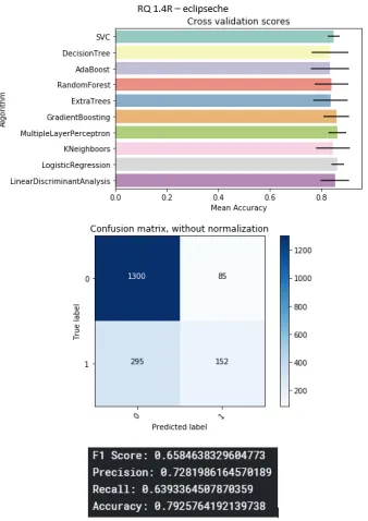
B.2.1 RQ1: . . . 78
Repository metrics: . . . 78
Code metrics: . . . 84
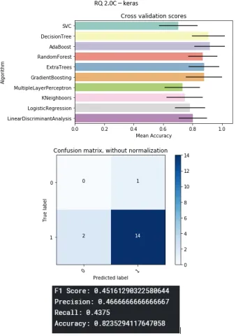
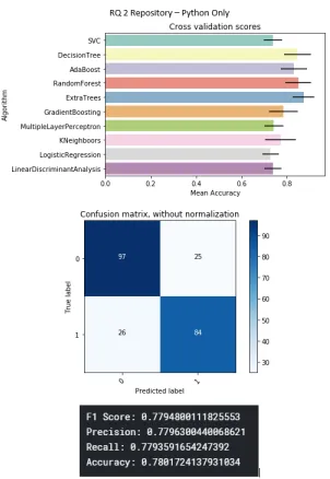
B.2.2 RQ2: . . . 89
Repository metrics: . . . 89
Code metrics: . . . 90
B.2.3 RQ3: . . . 91
Repository metrics: . . . 91
Code metrics: . . . 92
B.2.4 RQ4: . . . 93
Repository metrics: . . . 93
Code metrics: . . . 94
B.2.5 Validation: . . . 95
RQ2: . . . 95
Curriculum Vitae 97
List of Figures
2.1 Overview of Github’s [1] API Data Model . . . 12
3.1 Overview of project selection, research questions, experiment and validation . . 23
3.2 Fractal visualization example [77] . . . 24
3.3 Sum of Coupling visualization example [77] . . . 25
3.4 Data collection from [1] using metrics tools [4, 8]. . . 27
3.5 Sample data with repository metrics. . . 29
3.6 Sample data with code metrics. . . 29
3.7 Imbalanced classes for springboot project . . . 31
4.1 Advanced Code Metrics . . . 41
5.1 Kopete and K3b detailed reports . . . 46
6.1 Code Debt example [73] . . . 53
6.2 Code Debt example [73] . . . 54
B.1 Overview of project selection, research questions, experiment and validation . . 78
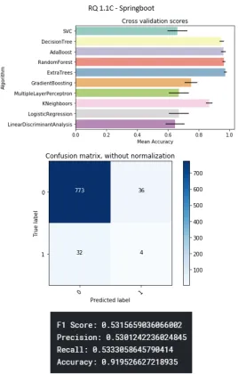
B.2 Springboot project . . . 79
B.3 Deeplearning4j project . . . 79
B.4 Elasticsearch project . . . 80
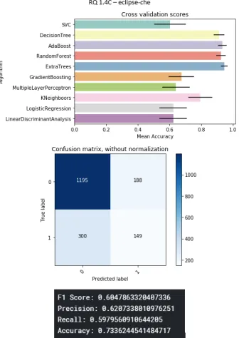
B.5 Eclipse-che project . . . 80
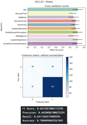
B.6 RxJava project . . . 81
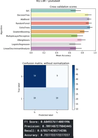
B.7 Youtube-dl project . . . 81
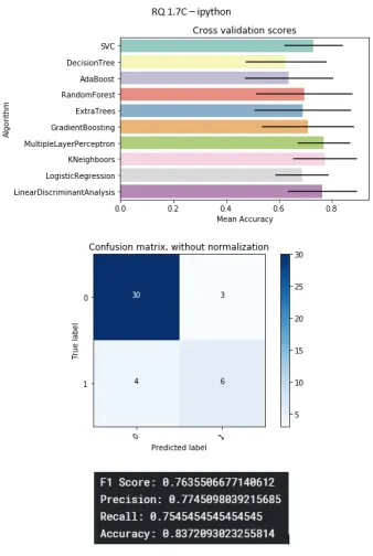
B.8 Ipython project . . . 82
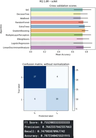
B.9 Scikit project . . . 82
B.10 Scrapy project . . . 83
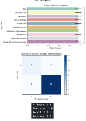
B.11 Keras project . . . 83
B.12 Springboot project . . . 84
B.13 Deeplearning4j project . . . 84
B.14 Elasticsearch project . . . 85
B.15 Eclipse-che project . . . 85
B.16 RxJava project . . . 86
B.17 Youtube-dl project . . . 86
B.18 Ipython project . . . 87
B.19 Scikit project . . . 87
B.20 Scrapy project . . . 88
B.21 Keras project . . . 88
B.22 Repository metrics on java projects only . . . 89
B.23 Repository metrics on python projects only . . . 89
B.24 Code metrics on java projects only . . . 90
B.25 Code metrics on python projects only . . . 90
B.26 Repository metrics with java as test project . . . 91
B.27 Repository metrics with python as test project . . . 91
B.28 Code metrics with java as test project . . . 92
B.29 Code metrics with python as test project . . . 92
B.30 Repository metrics with java as test project . . . 93
B.31 Repository metrics with python as test project . . . 93
B.32 Code metrics with java as test project . . . 94
B.33 Code metrics with python as test project . . . 94
B.34 Kopete detailed report using Python projects . . . 95
B.35 K3b detailed report using Python projects . . . 95
B.36 Kopete detailed report using Java projects . . . 96
B.37 K3b detailed report using Java projects . . . 96
List of Tables
2.1 Confusion Matrix . . . 9
3.1 Systems used in the experiment. . . 23
4.1 Repository metrics Before re-sampling and After re-sampling. . . 34
4.2 Code Metrics Before re-sampling and After re-sampling. . . 35
4.3 Example for Aggregated method. . . 35
4.4 Superimposed (Repository and code metrics) - Before and After re-sampling. . 36
4.5 Predicting for Java project (springboot) and Python project (scikit) using repos-itory metrics. . . 37
4.6 Predicting for Java project (springboot) and Python project (scikit) using code metrics. . . 38
4.7 Predicting for Java project (springboot) and Python project (ipython) using repository metrics. . . 38
4.8 Predicting for Java project (springboot) and Python project (ipython) using code metrics. . . 39
4.9 Predicting bugs by partitioning each project of same language into train and test data. . . 40
4.10 Advanced Code Metrics . . . 42
4.11 Predicting for Java project (springboot) and Python project (scikit) using ad-vanced code metrics. . . 42
4.12 Predicting for Java project (springboot) and Python project (ipython) using ad-vanced code metrics. . . 43
4.13 Predicting bugs by partitioning each project of same language into train and test data. . . 43
5.1 Systems used in validating the experiment. . . 44
5.2 Comparing results of data validation on C++ projects with RQ3 repository metrics results. . . 45
5.3 Comparing results of data validation on C++ projects with RQ2 repository metrics results. . . 46
5.4 Comparing results of data validation on C++ projects with RQ2 repository metrics results. . . 47
6.1 Summary of the discussion . . . 49
Chapter 1
Introduction
1.1
Introduction
Before any software application is delivered to the clients, it has to be tested so that it is verified that it meets its functional and non-functional requirements. Software testing is often paired with software reliability prediction models, so that the overall testing time required for the system to reach a specific failure intensity level can be estimated. However, for many non-mission critical applications which nevertheless have strict time to market constraints or the strict release deadlines, we often require the use of a triage method in order to prioritize testing depending on the estimated risk of failure of each software module on the application being tested. For many systems (e.g. mobile applications) short release cycles make the testing of every possible execution path not feasible, while meeting at the same time strict release deadlines. In this respect, we need to devise a technique by which we can alert both developers and testers regarding the risk of failure of a software component. This will help to appropriately schedule and prioritize the test cases to be applied. In this thesis, we conduct and report results from a series of experiments in order a) to investigate whether machine learning can be a feasible approach towards developing models for evaluating the fault proneness of a software module and b)identify a number of source code and non-source code related features which may be of use towards training the aforementioned models.
The main focus of this thesis is to devise fault prediction models, so that software develop-ers and software testdevelop-ers can obtain an initial view on how to manage and prioritize testing in large software systems. More specifically, given a software systemS, a commit actionCi in-volving a collection of revised filesRi={F1,i,F2,i,. . . Fk,i}, and a trained modelMon a history of revisions and system metricsH, we would like to be able to predict which of the files Fj,i are fault prone, so that a) developers can be alerted for possible impeding failures of the file(s) they have revised; b) testers can prioritize and re-schedule their test plans so that fault prone modules can be tested first, and; c) managers can be alerted for possible failure risks. The sys-tem can serve as a first step on a larger pipeline that supports continuous software engineering (integration, release, and deployment) by providing insights for automating DevOps processes. More specifically, in this thesis we present a framework for training and applying machine learning models for the purpose of evaluating the likelihood of a file being fault prone. In this study we use source code metrics as well as non-source code information obtained from
2 Chapter1. Introduction
ous repositories (e.g. number and frequency of commits, past failures, refactoring operations), in order to train the machine learning framework. In this thesis, and according to IEEE termi-nology [63] we use the term faultto indicate an incorrect step, process, or data definition in a computer program (i.e a bug). Afault may cause anerror which is a difference between a computed result and a correct result and it is internal to the state of the program. Consequently, anerrormay cause afailurewhich is a deviation of the expected behavior of the program from theobservedone.
In this thesis, we have collected data from five Java and five Python open source systems that are available on GitHub[1], as illustrated in Table 3.1. We have selected parts of these systems to train a number of fault proneness prediction models, and we have consequently applied these models on the rest of the aforementioned systems. As an additional validation and in order to prove the generality of the prediction models, we have applied the best performing prediction models on two large open source C++systems obtained from the KDE repositories.
1.1.1
Problem Area and Motivation
Problem Area: Software Analytics for the identification and assessment of fault proneness of a software system at the file level.
Motivation: Most of the software applications are almost certain to produce failures due to faults (bugs) introduced during the development or maintenance phases. A good number of these errors are discovered by the testing team and few of them are discovered over time in the operational phase.
However, it has been reported that the cost of fixing a bug in later stages of the software development cycle can be very expensive when compared to the development phase [70, 15]. Therefore, one must take this into account and try to find and fix bugs as early as possible.
The simplest way to find bugs is by testing. In [53] software testing is defined as ‘the process of executing a program with the intent of finding errors‘. There are different types of testing as described in [13] such as unit testing, function testing, system testing and integration testing.
It has been observed that most of the time the testing activities consume anything between 45% to 75% of the total development time [25]. By providing predictions on whether a file contains a fault or not, we may be able to reduce the amount of time consumed during the testing phase by focusing first on the probable buggy files. With respect to bug prediction, there have been many studies since 1970’s ranging from simple equations for measuring code complexities [30] to machine learning algorithms [20, 35].
1.1.2
Contributions, Scope and limitations
1.1. Introduction 3
with a standardized set of features and a standardized set of pre-processed data so that these can be used to train such Machine Learning frameworks in order to yield predictive models. This thesis falls in the area of Experimental Software Engineering, and aims to shed light in the problem of identifying such a collection of Machine Learning frameworks, repository fea-tures, and software metrics that can be used for the generation of fault prediction models. The objective is to provide experimental data points for software engineers and computer scientists to use towards developing more and more accurate predictive models. The thesis focuses on the analysis of ten large open source systems by considering a volume of more than 75,000 issue-bearing commit records. The thesis contributions can be summarized as follows:
• Investigate and report on the effectiveness of selected features and metrics to be used for language agnostic software fault proneness prediction at the file level;
• Investigate different Machine Learning frameworks and their effectiveness on yielding fault prediction models, and;
• Investigate five key research questions RQ1-RQ5 (please see section below) that can shed light on the effectiveness of the predictive models under different operational scenarios.
The thesis is comprised of:
• A tool for extracting repository metrics [8] from GitHub.
• A tool for extracting source code metrics for Java and Python projects [4].
• Custom made Java application programs (Appendix A.1.1,A.1.2) for combining the met-rics and bug reports into a desired format.
• Use of existing open source infrastructure provided by Kaggle [2] in conjunction with the use of custom made programs to train and evaluate prediction models.
• The analysis, discussion, and explanation of the obtained results.
This thesis, however, does not address whether the models have similar performance to different types of applications (e.g real-time systems, enterprise systems, systems that depend on scripting languages). Furthermore, the thesis does not take into account lower level source code dependencies or other low level source code related information (e.g. information ex-tracted from the AST).
1.1.3
Research questions
In this work we aim to find and report on empirical evidence to answer the following research questions, which constitute a typical set of research question found in the related literature. RQ1a: Is it possible to train models that can be used to predict fault-proneness of individual projects, by using repository and source code metrics?
4 Chapter1. Introduction
RQ2: Given a set of projects{P1,P2,P3....,Pn}, written in a languageL, is it possible to train the model on all projects{P1,P2,P3....,Pn−1}in order to predict fault proneness for projectPn?
RQ3: Given a set of projects{P1,P2,P3....,Pn}, written in languages L = {L1,L2,L3....,Lk} is it possible to train the model on all projects{P1,P2,P3....,Pn−1}in order to predict bugs for projectPnwritten in a languageLi ∈ L?
RQ4: Given a set of projectsP={P1,P2,P3....,Pn}, written in the same languageL, is it pos-sible to predict fault proneness of a projectPi ∈ Pby partitioning the projects{P1,P2,P3....,Pn} into two sets, one set (80%) for training the model and the other set (20%) for predicting fault proneness?
RQ5: Using advanced code metrics, answer RQ1, RQ2, RQ3 and RQ4. Do advanced code metrics improve the results?
1.1.4
Thesis outline
Chapter 2
Background and related work
2.1
Background
2.1.1
Code Metrics
Static code metrics are metrics which can be extracted directly from the source code, such as the total number of lines of code (LOC), Halstead metrics, Henry-Kafura metrics, and cyclo-matic complexity metrics. One such static code metric is the Source Lines of Code (SLOC) which represents a related family of metrics focusing on counting lines in a source code file. Among others, the SLOC family includes, the total number of blank lines (BLOC), the total number of lines in a file (LOC), the total number of commented lines of code (CLOC), and the total number of the logical lines of source code (SLOC-L) which is the total number of executable lines of code [57, 5, 6]. The Cyclomatic Complexity (CCN), also known as the McCabe metric or the McCabe Cyclomatic Complexity, is a measure of the complexity of the decision structure, in the control flow graph of the code of a module. The metric introduced by Thomas McCabe [49] and is equal to the number of linearly independent paths in the control flow graph [49].
SR Chidamber et al. in [23] and J Bansiya et al. in [12] discuss object oriented metrics such as the:
1. Weighted Method per class (WMC), which is the number of methods in the class [23].
2. Depth of inheritance Tree(DIT) which measures the inheritance levels from the top of the hierarchy of objects for each class. [23].
3. Number of Children (NOC)which measures the number of the class’s immediate descen-dants [23].
4. Coupling between Objects (CBO)which is a metric that represents the number of classes coupled to a class. The coupling can be achieved through method calls, field accesses, inheritance, method arguments, return types and exceptions. [23].
5. Response for a class (RFC)which is the number of Distinct Methods and Constructors invoked by a class [23].
6 Chapter2. Background and related work
6. Lack of Cohesion of methods (LCOM):If ’m’ is the total number ofmethodsin a class and ’a’ is the total number ofattributesin the class then LCOM is computed as follows: 1 – (sum(am)/a*m) where ’am’ is the number of methods accessing a particular attribute and ’sum(am)’ is the total sum of ’am’ over all the instances in the class [23, 3].
7. Number of Public Methods (NPM)which is a metric that counts all the methods in a class that are declared as public [12].
8. Data Access Metric (DAM) which is a metric that is the ratio of the number of private attributes to the total number of attributes declared in the class [12].
9. Measure of Aggregation (MOA)which is a metric that measures the extent of the part-whole relationship (aggregation, composition), realized by using attributes. The metric is a count of the number of class fields whose types are user defined classes [12].
10. Measure of Functional Abstraction (MFA)which is the ratio of the number of methods inherited by a class to the total number of methods accessible by the member methods of the class [12].
11. Cohesion Among Methods of Class (CAM)which computes the relatedness among meth-ods of a class based upon the parameter list of the methmeth-ods. The metric is computed using the summation of a number of different types of method parameters in every method, di-vided by a multiplication of number of different method parameter types in whole class and number of methods [12].
2.1.2
Machine Learning
2.1. Background 7
Support vector machine for classification (SVC): Support vector machines (SVM) have been proposed by Vapnik [79] along with other researchers, and they have been widely studied and applied in many fields. The basic idea of SVM is to to identify a similarity distance between two entities (classes) by considering a distance metric between them. The distance between such entities (classes) is traditionally defined as a function of their feature vectors [39]. Support Vector Machine could also be used to accommodate for unbalanced classes[61]
Decision tree: Decision tree classifiers use comparisons to divide different instances of a set into appropriate classes. Classification is a type of supervised learning where initially, a set of known instances, called the training set, is introduced to a system. The system classifies each instance of the set, associates each class with the attributes of each instance and learns to what class each instance belongs. Based on what the trained system has learned in the learning phase, it is able to classify instances of a previously unseen set [74].
One application of using Decision trees is for pattern recognition algorithms [74]. Another application of this type of Machine Learning is image analysis such as in cancer cell and brain tumor detection [21].
AdaBoost: As described in [10], the AdaBoost algorithm is one of the most well-known al-gorithms for building anensembleclassifier. Each instance in the training dataset is weighted. The initial weight is set to: weight(xi) =1/n, where xi is the ith training instance and n is the number of training instances. The most common algorithm used with AdaBoost aredecision treeswith one level. As these trees are short and contain only one decision for classification, they are called asdecision stumps. A weak classifier (decision stump) is prepared on the train-ing data ustrain-ing the weighted samples. The AdaBoost algorithm generates a strong classifier by adjusting weights through a repetition process[24].
Random forest: Breiman [16] suggested a new and promising classifier in (2001) called random forest, which presents many advantages [32] such as its running efficiently on large databases, being able to handle thousands of input variables, and providing estimates indicating which variable is important in a classification session.
8 Chapter2. Background and related work
Evaluating machine learning models
Accuracy: Accuracy (equation 2.1), measures the proportion of the files classified correctly, to the total number of files. Accuracy, however omits a detailed analysis such as the number of correct labels of different classes [72] and in this respect researchers in order to evaluate the model also use the F1 Score as well as precision and recall which are described below.
Acc= true positives+true negatives
true(positives+negatives)+ f alse(positives+negatives) (2.1)
Precision: Precision (equation 2.2) measures the proportion of files that were correctly clas-sified as faulty over the total number of files clasclas-sified as either faulty or non-faulty. In other words, Precision or Confidence (as it is called in Data Mining) denotes the proportion of Pre-dicted cases that are indeed real faulty files [62]. This is a measure of how good a prediction model is at identifying actual faulty files.
Precision= true positives
true positives+ f alse positives (2.2)
Recall: Recall (equation 2.3) measures the proportion of faulty files which are correctly iden-tified as faulty over the total number of faulty files available. Recall or Sensitivity (as it is called in Psychology) is the proportion of real faulty files that are correctly predicted as faulty files[62].
Recall= true positives
true positives+ f alse negatives (2.3)
F1Score: TheF1Score is computed by taking the (weighted) harmonic average of precision and recall as shown in equation (equation 2.4).
F1S core=2∗
Precision∗Recall
Precision+Recall (2.4)
2.1. Background 9
actual value
Prediction outcome
p n total
p0 True Positive
False
Negative P 0
n0 False Positive
True
Negative N 0
total P N
Table 2.1: Confusion Matrix
2.1.3
Technical Debt
Thetechnical debtmetaphor was first defined by Ward Cunningham in 1992, where most cited words were ‘not quite right code’ [26]. The definition followed many extensions referring to how the software development teams chose to delay certain maintenance tasks in favor of quick and easy fixes while running the risk causing problems in the future. Therefore, the team opts for an easy and quick way to implement a feature or a fix to a bug in the shortest possible time but with greater chances of negative impact in the long run.
Technical debtrefers to the debt incurred by any software item that is inappropriate or deviates from standards and which is included in the system due to urgent fixes or lack of time to properly design the system or lack of time to re-factor it. For example: missing or inadequate documentation, not restructuring or re-factoring complex code, not executing the planned test cases, known defects or bugs that are not yet fixed, etc. Below we provide a list of different types of technical debt.
Architecture Debt
This type of debt refers to the type of issues related to the project architecture [46, 76].
Example: Lack of modular components that affect functional or non functional requirements such as poor performance, robustness, etc.
Identification: The way to identify this type of technical debt is through structural analysis, analysis of component dependencies at the architectural level, and identification of modularity violations [9].
Build Debt
10 Chapter2. Background and related work
Example: Use of too many external libraries could result in build debt.
Identification: The way to identify this type of technical debt is by performing a dependency analysis between the different modules, and the use of dependencies due to libraries or the use of externally linked modules [9].
Code Debt
This type of technical debt is found in the source code of projects that do not follow good coding practices. This practice generally makes it difficult to maintain and in worst cases could lead to rewrite of the entire project or module. Code debt could be handled using static code analysis tools [76, 87].
Example: Using wrong naming conventions in variables or using code cloning.
Identification: The way to identify this type of technical debt is by searching for duplicated code, slow or complex algorithms, code written in a way that violates standards, and by ana-lyzing code metrics [9].
Defect Debt
This type of debt is incurred when a bug is logged in the bug tracking system of the project, generally by the testing team but is deferred due to other high priorities or limited resources available to fix the bug [71].
Example: Defer bug fixes to next cycle in order to meet the current project release deadline. Identification: The way to identify this type of technical debt is by analyzing bug tracking systems to locate uncorrected known defects [9].
Design Debt
This type of debt is incurred when a project ignores the principles of object oriented design thereby resulting in either large classes (God Classes) or tightly coupled classes [76, 87]. Example: Frequently used code could be generalized using parameters instead this block of code is duplicated across the entire project.
Identification:The way to identify this type of technical debt is by analyzing the system for unusual code metrics patterns, code smells, dispersed coupling, duplicated code, god classes, intensive coupling, and issues in the software design [9].
Documentation Debt
This type of debt is incurred in a project when there is missing, incomplete or inadequate doc-umentation. [76, 66]
2.1. Background 11
Identification: The way to identify this type of technical debt is by analyzing system docu-mentation, incomplete design specifications, insufficient comments in code and outdated doc-umentation [9].
Test Debt
This type of debt is incurred in a project when certain planned test activities that affect the testing quality are ignored [76, 66].
Example: Skipping certain planned test cases, unable to meet the planned test code cover-age.
Identification: The way to identify this type of technical debt is to analyze the system for incomplete tests and low test coverage [9].
Requirement Debt
This type of debt is incurred in a project when there is a trade-offas to what requirements the development team needs to implement versus the time to release or versus the project’s budget [46].
Example: Partially implemented requirements, incomplete requirements.
Identification: The way to identify this type of technical debt is by examining the require-ments backlog list [9].
Infrastructure Debt
This type of debt is incurred when there is an infrastructure issue that could hinder the devel-opment activities. [67]
Example: Infrastructure failure.
Identification:The way to identify this type of technical debt is to examine the underlying infrastructure (e.g. the middleware) for suitability towards meeting the system’s functional or non-functional requirements.
People Debt
It refers to people issues that could delay or hinder the software development activities. [76, 67] Example: Few subject matter experts, delay in training.
12 Chapter2. Background and related work
debt[76, 87],defect debt[71],design debt[76, 87],documentation debt[76, 66], andtest debt [76, 66], here we only focus oncode debtanddefect debt.
2.1.4
GitHub
Figure 2.1: Overview of Github’s [1] API Data Model
GitHub [1] is a web-based hosting service for version control using Git and it is the preferred repository hosting service for many open source projects. Interestingly, GitHub provides an extensive REST API (5000 calls/hour for authenticated users), thereby, making it attractive for researchers.
2.2. RelatedWork 13
ofCommit orIssueorPullRequest. Theid is a common attribute for all the entities which is a unique identifier except forCommit which hasshaattribute as its unique attribute. When a Usercommits a file, a unique ID which is known as ”sha” or ”hash” is created.
TheUser entity contains user information such as thelogin, name, email, count of public repositories (public repos), etc. The Repoentity containstypeattribute whose value could be a ’file’, ’user’, ’symlink’ or ’submodule’ and the contentis set respectively. For example, if the value of typeattribute is ’file’ then content attribute stores its respective data (usually by base64encoding). TheIssueentity contains information related to all the issues encountered with the project. It has a reference toPullRequest which is used to let User know about the changes made to repository.PullRequestis associated with zero or morePullRequestComment which contains the attributecommits.
2.2
Related Work
2.2.1
Software Bug Prediction using Machine Learning
There is a variety of machine learning methods that have been proposed for addressing the software bug prediction problem. These methods include decision trees [44], neural networks [91, 75], Naive Bayes [50, 78, 37], support vector machines [33], Bayesian networks [58] and Random Forests [19].
R Malhotra in [48], conducted a systematic literature review of the software bug prediction techniques in 64 primary studies and concluded that the most used machine learning techniques are:
1. Decision trees (DT)
2. Bayesian learners (BL)
3. Ensemble learners (EL)
4. Neural networks (NN)
5. Support vector machines (SVM)
6. Rule based learning (RBL)
7. Evolutionary algorithms (EA)
8. Miscellaneous Approaches
Also, in [48], R Malhotra identifies that the most commonly used metrics for predicting fault proneness are divided into four categories as follows:
14 Chapter2. Background and related work
2. Object-oriented metrics: These approaches use metrics that measure various object ented software attributes such as cohesion, coupling and inheritance for an object- ori-ented class. In addition to object oriori-ented metrics, these approaches also use LOC type of metrics adjusted for the object oriented nature of the code (e.g. taking into account inheritance).
3. Hybrid metrics: These approaches use both object- oriented metrics and procedural met-rics to predict fault proneness.
4. Miscellaneous metrics: Metrics such as requirement metrics, change metrics, network metrics extracted from the dependency graph, churn metrics, defect slip through metrics, process metrics, age of file, size, changes and defects in previous versions, elementary design evolution metrics and other miscellaneous metrics that can not be grouped as ei-ther procedural or object-oriented metrics, are tagged under Miscellaneous metrics [48].
The object-oriented metrics that are shown to be correlated to fault proneness are CBO (cou-pling between objects), RFC (response for a class) and LOC [48]. The other metrics that are correlated are WMC, NPM and LCOM. For procedural metrics, the studies do not yield a conclusive result.The results obtained from the primary selected studies indicate that the NOC (number of children) and DIT (depth of inheritance tree) as not useful metrics [48].
R Malhotra [48], identified also the most commonly used metrics to measure performance of the models as well as, the mean performance of these models. More specifically, the study identified that the most commonly used performance metric is Recall which is closely followed by Accuracy, Precision, AUC measures, Specificity, Pf, and Fmeasures. Some less commonly metrics are grouped in the miscellaneous category namely Hmeasure, Precision-recall curve and error rate. The results are provided in the 64 primary studies had the mean values of accuracy ranging from 0.75 to 0.85.
The work in [48] examined also the prediction capability of the machine learning tech-niques for classifying a file as buggy or not buggy. The machine learning models for estimating software fault proneness outperform the traditional probability models. Based on the results obtained from the systematic review, they also conclude that the machine learning techniques have the ability for predicting software defects and can be used by software practitioners and researchers. However, the machine learning techniques in software bug prediction is still in its initial stages and very limited, and more work should be carried out [48, 80].
HK Dam et al. in [27], performed software defect prediction on two datasets, one from open source projects provided by Samsung and the other, from the public PROMISE repository with a total of 10 Java projects. HK Dam discusses the implementation of a deep learning, tree-structured Long Short Term Memory network which maps with the Abstract Syntax Tree representation of the source code. The entire process is based on three steps.
The first step is to parse a source code file into an Abstract Syntax Tree(AST). The second step is to map the AST nodes into continuous-valued vectors called embeddings and then input these embeddings to a tree-based network of LSTMs to get a vector representation of the whole AST. The third step is to input this vector into a traditional classifier (e.g. Logistic Regression or Random Forests) to predict defect outcomes.
2.2. RelatedWork 15
and average AUC of 0.6. For cross-project prediction, their approach did achieve a very high recall, with an average of 0.8 across 22 cases. The average F-measure was reported 0.5 but the approach suffered from low precision.
Xinli Yang et al. in [85], performed defect prediction experiments on 6 large-scale soft-ware projects from different communities, i.e., Bugzilla, Columba, JDT, Platform, Mozilla, and PostgreSQL. The authors present the overall framework of their proposed approach called ’Deeper’ which is summarized as follows. The procedure consists of two parts: a model build-ing phase and a prediction phase. In the model buildbuild-ing phase, the goal is to build a classifier by using deep learning and machine learning techniques from historical code changes. In the pre-diction phase, this classifier would be used to predict if an unknown change would be buggy or clean. In [85], Xinli Yang et al. used 14 basic features such as the number of modified subsys-tems, directories, files, the number of lines added, deleted, total lines of code and developer’s experience to train their model. The results obtained using the ’Deeper’ model indicate that the best the model could do in terms of precision, recall and accuracy are 0.55, 0.72 and 0.62 respectively.
W´ojcicki et al. in [83], want to verify whether the type of approach used in former fault prediction studies can be applied to Python and opted for using a Na¨ıve Bayes classifier for fault prediction. The model used McCabe’s cyclomatic complexity measure, counters of operators and operands (Halstead metrics) as features. The results achieved recall up to 0.64 with a false positive rate of 0.23. The mean recall and mean false positive rate were reported as 0.53 and 0.24 respectively.
Venkata et al. in [22], compared different machine learning models for identifying faulty software modules and they found that there is no particular learning technique that performs the best for all the data sets. In that study, the metrics used were McCabe, Halstead, line count, operator and branch count. The models used were Decision Trees, Na¨ıve-Bayes, Logistic Regression, Nearest Neighbor, 1-Rule and Neural Networks. Venkata et al. in their results show that the “size” related and “complexity” related metrics are not sufficient attributes for accurate prediction, and they need to include dependencies between these metrics to improve the prediction models.
Wang and Yao in [81], aimed to find bugs without decreasing the overall performance of the model. In their study, the machine learning algorithms used were Naive Bayes (NB), and Random Forest (RF). The dataset used for training the model is taken from public PROMISE repository. In this process, they find that imbalanced distribution between classes in bug pre-diction is the root cause of its learning difficulty. Likewise, in our thesis, we noted the issue and used re-sampling as described in detail in the section 3.4.2.
16 Chapter2. Background and related work
2.2.2
Software Metrics
Object Oriented Metrics
DL Gupta et al. in [34] investigate and assess the relationship between different object-oriented metrics and defect prediction capability by computing the accuracy of their proposed model on different datasets obtained from different repositories for a given project. A total of 12 experiments were carried out on different dataset sources, using 14 different classifiers for each experiment. The metrics used to train the model are WMC, DIT, NOC, CBO, RFC, LCOM, CA, CE, LOC and LCOM3, NPM, DAM, MOA, MFA and CAM. The classifiers used are Naive Bayes, LivSVM (Support Vector Machine), Logistic Regression, Multi-Layer Perceptron, SGD (Stochastic Gradient Descent), SMO (Sequential Minimal Optimization), Voted Perceptron, Attribute Selected Classifier, Classification Via Regression, Logit Boost, Tree Decision Stamp, Random forest, Random Tree and REP (Reduce Error Pruning) Tree. On an average, 76% accuracy is achieved at testing (prediction) stage when training is done on all the datasets. It is concluded from all the experiments, that some datasets have similar prediction accuracy result, while some give different results for the same projects on other datasets. Similar conditions occur when training and testing are both done on all the datasets and this type of variation in the accuracy at prediction (testing) stage may be due to different softwares (datasets) used for the experiments.
K El Emam et al. in [29], based on the previous work on predicting faulty modules using object oriented design metrics, such as DIT, NOC and the Briand et al. coupling metrics (like CBO and RFC). To perform validation of object-oriented design metrics, a commercial Java system is used. The objective of the validation is to determine which of these metrics are asso-ciated with fault-proneness. The metrics used in the validation are DIT, NOC, ancestor-based coupling metrics and descendant-based coupling metrics. The results indicate that inheritance depth and coupling metric were strongly associated with fault-proneness. The prediction model with these two metrics has promising accuracy but only one system was considered for the ex-periment.
M Cartwright et al. in [18], investigated an industrial object-oriented module using em-pirical methods. The module has a size of 133 KLOC, is written in C++ and is part of a larger real-time European telecommunication product which comprises several million lines of code(LOC) and has been evolving over the past 10 years. The metrics used to experiment were LOC, the number of all read accesses by a class, the number of all write accesses by a class, depth of inheritance (DIT), number of child classes (NOC) and the number of defects of each class. The experiment that used the Shlaer-Mellor method [69] concluded that object-oriented constructs such as inheritance and polymorphism are not really useful to predict defects. Ac-cording to the authors in [18], the classes involved in inheritance structures were three times more defect prone than the classes that were not involved in inheritance structures. On the other hand, these results may be a consequence of the development method used, or the fact that the C++language does not enforce an object-oriented approach, or the fact that this was the project team’s first experience of object oriented development.
2.2. RelatedWork 17
Menzies et al. in [50] used static code metrics such as SLOC and CCN for defect prediction. According to Menzies et al, they observed that the prediction performance was not affected by the choice of static code metrics but by how the chosen metrics are used. Therefore, the choice of selecting and training a machine learning algorithm plays more an important role than the metrics used for training the machine learning algorithm. The authors, measure performance by using Probability Detection (PD) and Probability of False alarms (PF). Using a Na¨ıve Bayes algorithm with feature selection, they gained a PD score of 71% with PF at 25%.
Zhang et al. in [89] commented on them using PD and PF performance measures and pro-posed the use of precision and recall instead. Zhang [88] investigated if is a co-relation between LOC and defects on publicly available datasets. Zhang et al. argued that LOC when combined with machine learning classification techniques, could be a useful indicator of software qual-ity. The results are definitely interesting because LOC is one of the simplest and easy to collect software metric.
Repository Metrics
Repository metrics are also known as change or process metrics. Repository metrics are metrics that are based on historic changes made on source code over a period of time. These metrics can be extracted from version control systems. A few examples of repository metrics are the number of additions and deletions of lines from the the source code, total number of altered lines of code, the number of authors of a file, the number of commits a file, etc.
AE Hassan in [36], discusses how frequent source code “commits” in the repository, neg-atively affect the quality of the software system, meaning that the more changes incurred to a file, the higher the chance that the file will contain critical errors. Furthermore, Hassan in [36] presents a model which can be used to quantify the overall system complexity using historical code-change data, instead of plain source code features.
B Caglayan et al. in [17] discuss about the merits of using repository metrics for bug prediction and have concluded that repository metrics provide a better insight to the software product and lower the probability of false alarms. Moreover, the authors in [17] concluded that static code attributes provide limited information content. Software modules represented in terms of static code attributes may overlook some important aspects of software, including the type of application domain; the level of skills of the individual programmers involved in system development; contractor development practices; variation in measurement practices; and the validation of measurements and instruments used to collect the data [17]. There have been a few approaches that use repository data to predict defects but they did not consider the number of developers. They found that a high number of programmers coupled with commits to the same file, as well as a high temporal concentration of commits, were associated with class level quality problems, and in particular size and design guidelines violations [17].
Moser et al. in [52] compared the efficiency of using repository metrics for defect prediction to static code metrics. Their conclusion was that process data contained more information on the distribution of defects than the source code metrics. Their explanation is that the source code metrics concern the human understanding of the code. For example, large files of source code do not necessarily mean that the file is fault prone.
18 Chapter2. Background and related work
of time. Nagappan et al. concluded that the use of relative code churn metrics better predict the defect per source file than other metrics, and that code churn can be used to distinguish between defective and non-defective files. By relative churn measures the author takes into consideration the normalized values of the various measures obtained during the churn process. For example, a few of the normalization parameters are total lines of code, file churn, file count etc.
Ostrand et al. in [60] used repository metrics explaining whether a file was new and whether it was modified or not. The authors used these metrics in addition to other metrics and found that 20 percent of the files, identified by the prediction model as most fault prone, contained on average 83 percent of the faults.
Test Metrics
Test code metrics may consist of the same set of code metrics as described earlier, but their only difference is now that they are applied on the source code of the test classes. Adding to this, Nagappan et al. in [56] introduced a test metric suite called Software Testing and Relia-bility Early Warning metric suite (STREW) in order to find defects in software programs. In STREW, Nagappan et al. considered nine metrics belonging to three different families namely Test quantification metrics; Complexity and object-oriented metrics and; Size adjustment met-ric. Nagappan et al. conclude that the metrics used in STREW provide at an early stage of de-velopment an estimate of the quality of the software as well as the identification of fault-prone modules [56]. Further studies conducted by the authors indicated that the STREW metrics suite for Java systems (also know as ’STREWJ’) can effectively predict software quality.
Dependency Metrics
In the design phase of the software development life-cycle, the division of the workload of dif-ferent components can be decided. However, this division of tasks can influence the quality of the software. Therefore, tracking dependencies between source code files could be a possible predictor of fault-prone components. Schr¨oter et al. in [65] proposed a new approach for de-tecting source files and packages for fault prone code. The authors collected import statements for each source code file or package, and compared these imports to component failures. The authors concluded that the dependent components, determines the likelihood of defects. The results show that the collection of imports at package level results in a better prediction than at file level. However, the results on the file level still work better than random assumptions.
Hybrid metrics
2.2. RelatedWork 19
a static and repository set combined. They concluded that the combined set was carried out just as well as the repository set, indicating that static code metrics are not worth collecting.
Technical Debt Metrics
N Zazworka et al. in [86] compared four approaches for technical debt identification. A number of source code analysis techniques and tools have been proposed to potentially identify the code debt accumulated in a system. N Zazworka et al. also investigated whether technical debt, as identified by the source code analysis techniques, correlates withinterest indicatorsin the form ofincreased defect-proneness and change-proneness. The selected four techniques for the analysis are identification of code smells, application of static analysis, identification of grime buildup (non design pattern related code which is included in the code that implements a design pattern), and modularity violations. The four techniques are applied to 13 versions of the Apache Hadoop open source software project to calculate technical debt. The indicators used in each of the techniques are: 1) Grime - Presence of Grime, Absence of Design Pattern; 2) Code smells - class level code smells such as God class and method level code smells such as coupling; 3) Source code analysis techniques - Finding bugs by priority (High, Medium, Low) and by category (Performance, Security, Experimental) and, 4) Modularity violations -Is there any presence of modularity violation?
N Zazworka et al., in his study, had the following observations:
• The value of technical debt indicators (Modularity violations, Grime, Code Smells and Source code analysis techniques) increases together with the size of the project.
• As for correlations between technical debt indicators and interest indicators (defect prone-ness and change-proneprone-ness), dispersed coupling points to classes that are more defect prone.
• Lastly, defect-prone classes also tend to be change-prone and vice versa.
J Xuan et al. in [84], proposes the concept of ’debt-prone bugs’ to model the technical debt in software maintenance. Debt-prone bugs are considered to be the debt incurred by maintenance operations, and produced by an incomplete or immature process of bug fixing and can add risks to software quality. Three types of debt-prone bugs, namely tag bugs, reopened bugs, and duplicate bugs were considered for examination. Three attributes were extracted for each of the types of debt-prone bugs. These are the number of bugs, the frequency of debt-proneness and the time of fixing bugs. To investigate the correlation between debt-prone bugs and product quality, prediction models were constructed based on historical information to predict the time related to fixing bugs.J Xuan’s et al. contributions can be summarized as follows.
20 Chapter2. Background and related work
bug tracking systems, but reopened later by another developer who realized that the bug was not fixed properly. The study showed that the time associated to fix reopened bugs is longer than the time associated for other bugs. These bugs are labeled as second type of debt-prone bugs. A Duplicate Bug is a new bug that has the same root cause in the bug tracking system as an existing bug. Ideally, duplicate bugs can be avoided if a developer is familiar with all existing and related bugs. However, in practice, developers can not check all existing bugs to determine whether a new bug matches an existing one. Since duplicate bugs are caused by the inadequate examination, these bugs are labeled as the third type of debt-prone bugs.
Finally, the authors in [84] conducted a case study to examine the correlation between debt-prone bugs and software quality in the Mozilla project. Their results indicated that the time related to fixing duplicate bugs can be seen as the strongest correlation factor to the average time of bug fixing. One possible reason for this, is that the duplicate bug ratio is greater than the other two types of debt-prone bugs. The Mozilla project experiment indicated also that the debt-prone bugs can help monitor and improve the quality of the software system.
2.2.3
Results Comparison
Chapter 3
Fault-proneness Prediction
In this chapter, we present a framework to utilize code and repository metrics in a machine learning environment in order to predict fault-proneness at the file level. Our study was con-ducted along three dimensions. The first dimension has to do with the selection of appropriate systems and appropriate code and repository metrics to use. The second dimension relates to the selection of the appropriate machine learning techniques. The third dimension deals with the training and evaluations of the models in several open source systems.
3.1
System Selection
3.1.1
Criteria
In [43], the authors document the results of an empirical study aimed at understanding the char-acteristics of the repositories and of users on GitHub. The empirical study talks in depth about mining GitHub for research purposes and how one should take various potential perils into consideration. The authors in their study listed 13 perils that were discovered. Our selection of projects from GitHub was based upon these perils. More specifically, our project selection was based on the following related criteria.
C1: A repository is not A project: The work in [43] concluded that a project is typically part of a network of repositories: at least one of them will be designated as central, where code is expected to flow to, and where the latest version of the code is to be found. Keeping this into consideration, we carefully selected projects that were not a part of a network of projects.
C2: Most projects have low activity or are inactive: Most of the projects have very low activity or are inactive [43]. Taking this into consideration, we only selected projects that had high activity in development, discussions and bug reports.
C3: Many repositories pertain to personal projects and do not relate to a major software application: Most of the projects stored in repositories relate to toy projects undertaken by developers [43]. Taking this into consideration, we selected project repositories that relate to open source software applications which are widely used.
22 Chapter3. Fault-pronenessPrediction
C4: Many active projects do not use GitHub exclusively and few projects use pull requests: Most of the projects do not use GitHub exclusively and only a few projects use pull requests [43]. It is true that very few projects use pull requests and therefore, it was very challenging to find large open-source projects that use pull requests. Of the projects we used for our study, all of them indicate a very high GitHub activity. However, we are unable to certify that GitHub was exclusively used in all of these projects.
C5: Only the user’s public activity is visible and GitHub’s API does not expose all data:The user’s public activity is visible and the API does not expose all the data [43]. For our experiment, we selected projects for which the data we needed were available.
3.1.2
Method
Figure 3.1 depicts the overall process of our framework. The first step relates to the selection of systems to be considered. We have selected a total of ten projects comprising five Java and five Python projects based on the criteria C1-C5 listed above. The second step relates to applying custom made programs to retrieve information pertaining to these projects from the corresponding GitHub repositories. The third step relates to modeling and reconciling the extracted information into a form that can be used by a machine learning framework. The fourth step relates to selecting ten different popular machine learning techniques (SVC, De-cision Tree, AdaBoost, RandomForest, ExtraTrees, GradientBoosting, MLP, KNN, Logistic Regression and LDA) so that models can be trained to answer question RQ1. Out of these ten models, we selected the five (SVC, DecisionTree, AdaBoost, RandomForest and KNN) top most performing models, based on their cross validation score (please see detailed report in Section B.1), in order to use these five models for answering the research questions RQ2 -RQ4. To answer the research question RQ5, this step was repeated but considering only ad-vanced source code metrics instead of our standard selected set of metrics. The fifth step relates to obtaining the best performing models from questions RQ2 and RQ3 and applying it to two C++projects obtained from KDE, in a quest to evaluate the applicability of our approach to systems written in a different language than the one the models were trained on.
3.1.3
Selected Systems
3.1. SystemSelection 23
Figure 3.1: Overview of project selection, research questions, experiment and validation
Table 3.1: Systems used in the experiment.
Project Name Language Files Lines of Code
spring-boot Java 4225 249,226
deeplearning4j Java 1845 498,447
elasticsearch Java 8460 1,087,149
eclipse-che Java 9159 704,659
RxJava Java 1604 273,053
youtube-dl Python 824 115,037
ipython Python 215 46,626
sci-kit Python 233 158,207
scrapy Python 240 27,439
24 Chapter3. Fault-pronenessPrediction
The selection criteria for the software applications to consider for our study were described in detail in Section 3.1.1. In addition to the selection process in Section 3.1.1, we also looked into the project size in terms of the number of files and lines of code. Larger systems were preferred over smaller ones in order to make the results more accurate and generalizable. We also looked at the availability of accurate information about software bugs and resolutions, so that the training and testing phases can be adequately supported. Lastly, we considered the overall complexity of the application as more complex applications entail a greater number of dependencies and opportunities for training. The software applications we considered in our study are listed in the Table 3.1 comprising of five Java and five Python systems, for which there is source code and repository related information available on GitHub (github.com) [1].
3.2
Metric Selection
3.2.1
Repository metrics
Fractal: This feature represents the percentage of code written by the original author that remains in the system after a series of commits over a period of time.
The fractal data provide another investigative tool to reveal files which undertook signifi-cant change compared to the original code. The visualization of fractal figures provides a view of how the programming effort was shared i.e. how fragmented the developer effort is for each module in a system[77]. An example is shown in Figure 3.2 where in file car.cpp, the value is 1 (i.e. all the code is the code of the original developer), while in file ClassShip.java the value is 0.25 indicating that only 25% of the original code remains.
3.2. MetricSelection 25
Sum of Coupling (SOC): Sum of couplingprovides information on how many times in total each module has been coupled to another one in a commit operation. For example, as depicted in Figure 3.3 the module app.clj is modified together with both module core.clj and module project.clj in commit #1, and module core.clj in commit #2. Therefore, its sum of coupling value is three. The premise is that the module that changes most frequently together with others, must be important and should a be good starting point for an investigation. There are different reasons for modules to be coupled. Some couples, such as a unit and its unit test, are valid. So modules with the highest degree of coupling may not be the most interesting to us. Instead, we want modules that are architecturally significant. A sum of coupling analysis helps locating those modules.
Figure 3.3: Sum of Coupling visualization example [77]
Age: This metric represents the age of the file in months.
Authors: This metric represents the total number of authors who have worked on the file.
3.2.2
Code metrics
Java code metrics: The code metrics used as features are described below.
26 Chapter3. Fault-pronenessPrediction
Based on McCabe‘s Cyclomatic Complexity, the complexity of the whole file is expressed as the number of independent control flow paths in it. It is calculated as the sum of the McCabe Cyclomatic Complexity values of the methods found in a file [5].
Comment Lines of Code (CLOC): It represents the number of comment and documentation lines in a source file [5].
Public Documented API (PDA): It represents the number of documented public classes and methods in a file [5].
Public Undocumented API (PUA): It represents the number of undocumented public classes and methods in a file [5].
Logical Lines of Code (LLOC): It represents the number of non-empty and non-comment code lines in a file [5].
Lines of Code (LOC): It represents the number of lines of code in a file [5].
Python code metrics: Similar to Java code metrics (excluding PDA and PUA), Python sys-tems have McCC, CLOC, LLOC, LOC and Number of Statements (NOS) as the features used to train the model.
Number of Statements (NOS): It represents the number of statements in the file [6]. These features were selected using Pearson’s correlation coefficient [14] and the tool that was used to plot Pearson’s correlation matrix was pandas’ correlation function and pyplot [40].
3.3
Data Collection Process
In order to collect data from GitHub, for both repository related information (e.g. commits, bugs, bug resolutions) and code metrics, a Java client program was developed and used in order to query GitHub as shown in Figure 3.4. The Java client program fetches every bug that was recorded for a file and keeps a count of the number of times it was found to contain an error (bug) that produced a failure. Other information that is fetched includes the number of source code commits, as well as the type of operation involved. The client program also connects with tools that compute source code metrics, and automatically populates a data base with all this information. Finally it performs data reconciliation, ensuring that the obtained data pertain to the same system, module and version. The bug data is then individually combined with the extracted repository metrics [8] and code metrics [4] to form two separate data files, one for predicting failures using repository features and another for doing the same using code metric features. The two individual results are then superimposed (intersected) to form one final result.
Below is the pseudo code (please see complete Java program in Section A.1.1) that is used to fetch all the bug reports from GitHub. The program is divided into three parts namely project configuration, bug data extraction, and finally exporting the extracted data to a csv formatted file.
In the first part i.e. project configuration, we connect using OAuth by providing the OAuth token that is acquired by creating an account on GitHub. Then, we specify the project name to connect and extract its details.
3.3. DataCollectionProcess 27
id, issue description, issue title and issue state are stored in a wrapper object.
In the third part of the program, all the data that we store in the wrapper class are now written into a csv file in order to combine these results with code and repository metrics. The algorithm for bug extraction is in Section A.1.1 and below is the pseudo code for the same.
Figure 3.4: Data collection from [1] using metrics tools [4, 8].
28 Chapter3. Fault-pronenessPrediction
Algorithm 1Pseudo code for bug extraction from GitHub
1: procedureIssuesSummary .This class is used to fetch all bugs from GitHub
2: Initialize oauthToken,GitHubBuilder,Github
3: Initialize GHIssue
4: Initialize GHLabels
5: .Config: To connect to GitHub, Initialize oauthToken,GitHubBuilder,Github
6: Initialize GHRepository .Initialize the Github repository to get the details
7: foreach in GHIssuedo
8: foreach in GHLabelsdo
9: GET IssueId, Body, Title, BugLabel, state
10: STORE IssueId, Body, Title, BugLabel, state in LIST
11: end for
12: end for
13: Write LIST to CSV .Write IssueId, Body, Title, BugLabel, State to csv file.
14: end procedure
Now that we have all the list of bug reports, the only way to link it with the files is to fetch all the commits for that repository, look for the issue id (if it exists as it could be an enhancement or a feature request) and map it with the files responsible for the issue. Below, we provide the pseudo code for the algorithm that extracts thecommitsfor the entire repository and maps the issue id with the files responsible for the issue (please see the complete program in Section A.1.2).
Pseudo code for combining extracted bug information with code and repository metrics: The pseudo code for combining extracted bug information from GitHub with code and reposi-tory metrics is shown in Algorithm 2,3. The complete Java code is in Section A.1.2.
Algorithm 2Pseudo code for commit extraction from GitHub
1: procedureCommitsSummary .This class is used to fetch all commits from GitHub
2: Initialize oauthToken,GitHubBuilder,Github
3: Initialize GHCommits
4: Initialize GHFiles
5: .Config: To connect to GitHub, Initialize oauthToken,GitHubBuilder,Github
6: Initialize GHRepository .Initialize the Github repository to get the details
7: foreach in GHCommitsdo
8: foreach in GHFilesdo
9: GET Date, Url, Message, Filename
10: STORE Date, Url, Message, Filename in LIST
11: end for
12: end for
13: Write LIST to CSV .Write Date,Filename,Url to csv file.
3.3. DataCollectionProcess 29
Algorithm 3Pseudo code for combining extracted bug information with code and repository metrics
1: procedureExtractIssueIdfromCommitsSummary.This class is used to map commits and bug reports from GitHub
2: Load CommitSummary.csv
3: whilecsvReader.hasNextdo
4: whilecommitHasBugdo
5: STORE Date,Filename,issueId,Message,Url in LIST
6: end while
7: end while
8: Write LIST to CSV .Write Date,issueId,Filename,Message,Url to csv file.
9: ADD respective metrics .Add Code or Repository metrics - this step is manual
10: end procedure
The bug report for each project is integrated with the corresponding metrics report obtained by the tools reported in [4, 8]. The integrated report was fed to Kaggle [2] in order to train and evaluate the models. The integrated bug reports with repository metrics is shown in Figure 3.5 and with code metrics, it is shown in Figure 3.6.
Figure 3.5: Sample data with repository metrics.
Figure 3.6: Sample data with code metrics.