Object Locating of Electromagnetic Inclusions in Anisotropic
Permeable Background Using MUSIC Algorithm
Faezeh Shirmehenji, Abolghasem Zeidaabadi-Nezhad*, and Zaker Hossein Firouzeh
Abstract—In this paper, a new formulation is proposed to solve an inverse scattering problem for locating isolated inclusions within a homogeneous noise-free and noisy biaxial anisotropic permeable background using MUltiple SIgnal Classification (MUSIC) algorithm. Locations of the dielectric, permeable, lossless and lossy electromagnetic or both dielectric and permeable inclusions with arbitrary ellipsoidal shapes can be restored. The numerical study of different inclusions is illustrated, and accuracy of the method is investigated. The proposed formulation is also investigated for extended inclusions backgrounds.
1. INTRODUCTION
Inverse scattering of electromagnetic waves is used in many applications such as the imaging of weather patterns, military radars, and nondestructive testing (NDT) such as the detection of a crack in a bridge [1–3]. Inverse scattering problems are investigated and solved by qualitative and quantitative methods. The qualitative methods yield shape and locations of the scatterers. The quantitative methods besides of shape and location give electromagnetic properties of scatterers, such as permittivity and permeability [3].
The MUltiple SIgnal Classification (MUSIC) algorithm which is a qualitative method is used only for point inclusions; however, multipath scattering between the inclusions is not taken into account by this algorithm. The transmitter and receiver antennas are in the far field of the inclusions. This algorithm also uses scattering waves to form multi-static response matrix. If the number of transmitter antennas is more than the number of inclusions, the required condition of MUSIC algorithm is provided [4]. This non-iterative algorithm needs less computation time than all of the quantitative methods. So, it can be used as an initial guess for the quantitative methods [5]. Another advantage of this algorithm is that it uses closed-form function for analysis.
In [6, 7] the MUSIC algorithm is employed to detect small two-dimensional cylinders. This approach cannot reconstruct the exact contour of large cylindrical scatterers, but it provides some information of them, such as the number of cylinders and their approximate location. In [8] and [9], this approach is used for imaging of the perfect conductor cracks; however, shape of the inclusions cannot be reconstructed. The MUSIC algorithm is also used to detect an inhomogeneous thin dielectric structure in a two-dimensional homogeneous space in [10] and electromagnetic structure in [11]. Time-Reversal MUSIC (TRM), investigated in [12–14] and [15], is used for multiple scattering among the scatterers, but it is not as simple as MUSIC. TRM imaging of extended targets has been investigated in [15].
In [16, 17] the locations of two and three dimensional ellipsoidal inclusions in free space are found, and the locations of three dimensional cubical inclusions are determined in an anisotropic background in [18] and ellipsoidal inclusions in [19].
Received 19 April 2018, Accepted 21 June 2018, Scheduled 6 July 2018 * Corresponding author: Abolghasem Zeidaabadi-Nezhad ([email protected]).
The macroscopic properties of an anisotropic electromagnetic material can be modeled by a tensor which describes dependency of the material permittivity and permeability on the wave direction. Anisotropic electromagnetic material can be modeled as a set of electric and magnetic dipoles with an arbitrary ellipsoidal shape in vacuum. The tensor of an anisotropic material is denoted by two 3×3 Hermitian matrices. These matrices can be transformed to diagonal matrices using rotation of the coordinates system as
[μ] =
μ
1 0 0
0 μ2 0
0 0 μ3
; [ε] =
ε
1 0 0
0 ε2 0
0 0 ε3
(1)
These matrices are used for biaxial materials, with triclinic structures such as mineral examples including microcline (KAlSi3O8), plagioclase with [μ] = μ0I3 where I3 is the 3×3 identity matrix. For uniaxial materials, such as the revolutionary ellipsoidal dipoles ε1 =ε2, [μ] = μ0I3, like Quartz. For spherical dipoles ε1 = ε2 = ε3, [μ] = μ0I3 and ε becomes a scalar, like Silicon and Gallium Arsenide [20]. Anisotropic magnetic materials are materials such as ferromagnetic materials including iron oxide (Feo3), composites, ceramic (BaO6Fe2O3), platinum cobalt (Pt, Co), cobalt samarium (Co, Sm) [21, 22]. For example [23]
[μ] =μ0
1.6664−0.0577i 0.0532 + 0.4425i 0
−0.0532−0.4425i 1.6664−0.0577i 0
0 0 1
(2)
In this work, we use the MUSIC algorithm to find the locations of small electromagnetic inclusions with both μ and ε as complex scalars with an arbitrary ellipsoidal shape, within a noise-free or noisy homogeneous biaxial anisotropic permeable background medium, with scalarεand second order tensor [μ]. The inclusions take the form of Iα = ∪mj=1zj +αBj, where Bj ⊂ R3 and zj ⊂ R3 are the boundary and location of the jth inclusion, respectively, and α is the common order of magnitude of the inclusions dimensions as a small fraction of the wavelength. Let for dielectric inclusions μα =μ0, εα = ε0, for permeable inclusions μα = μ0, εα = ε0, for electromagnetic inclusions μα = μ0,εα =ε0, for combination of dielectric and permeable inclusions μα =μ0, εα =ε0 orμα =μ0, εα =ε0, and for background [μb]=μ0I3,εb =ε0.
2. FORMULATION OF DIRECT PROBLEM
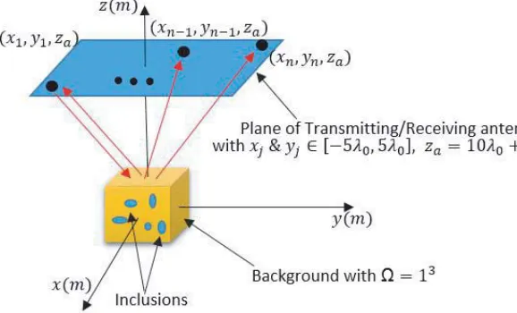
We firstly solve the direct problem. The inclusions are illuminated by several antennas, and then the scattered fields are evaluated as scattering matrix, Aα. The transmitting and receiving antennas are located in the constant z plane, z = za, with different (xi, yi), i = 1,2, . . . ,√n. The inclusions are illuminated by transmitting antennas, and the scattered field is measured by all receiving antennas. In fact, we have mono/multi-static conditions. To find the locations of electromagnetic inclusions in an anisotropic permeable background as shown in Fig. 1 for the background, we have [24]
⎧ ⎪ ⎪ ⎪ ⎪ ⎨ ⎪ ⎪ ⎪ ⎪ ⎩
Bb=μ0
H(0n)(r)I3+Mb =μ0
H(0n)(r)I3+χmbH(0n)(r) χmb =μrb−I3
Mb =μrb−I3
H(0n)(r) =ρ·H(0n)(r)
ρ=μrb−I3
(3)
where χmb, μrb, and Mb are magnetic susceptibility, relative permeability tensor, and magnetization vector of the anisotropic magnetic background, respectively, and H(0n)(r) is the incident magnetic field at the position rdue to thenth magnetic dipole element, directed in ˆβn as
M(0n)(r) =−iωμ0δ(r−rn) ˆβnIs (4)
where constant Is is the magnetic moment. The incident electric field from the dual problem of the preceding problem is given in [17] as
E(0n)(r) =iωμ0
I3+ ∇∇ k2
Figure 1. Configuration of the problem.
whereJ(0n)(r) is the current element, and
gr,r= e
ik|r−r|
4π|r−r| (6)
is a scalar function. To obtain H(0n)(r), since partial differential equation of H(0n)(r) is the same as
E(0n)(r), using duality theorem [17] it is enough thatEby H,HbyE,μby−ε,εby−μ, andJby−M
are replaced in Eq. (5)
H(0n)(r) =iωε0
I3+∇∇ k2
gr,r·M0(n)(r) =k2Is
I3+ ∇∇ k2
g(r,rn)·βˆn (7)
We define the dyadic Green’s function Gas
Gr,r=
I3+∇∇ k2
gr,r (8)
Using Eqs. (7) and (8),H(0n)(r) the scattered field at rdue to M(0n)(r) at position of rn is obtained as
H(0n)(r) =iωε0G
r,r·M(0n)(r) =k2IsG(r,rn)·βˆn (9)
By considering that ∇ ×H(0n)(r) =−iωε0E(0n)(r) we have
E(0n)(r) =iωμ0Is∇ ×G(r,rn)·βˆn (10)
According to Eqs. (3) and (9),Mb(r) becomes
Mb(r) =k2Is ρ·G(r,rn)·βˆn (11) LetHb(r) be the scattered field at position of rdue to Mb(r), therefore
Hb(r) = iωε0G
r,r·Mbr=iωε0k2IsG
r,r·ρ·Gr,rn·βˆn (12)
Eb(r) = −∇ ×Gr,r·Mbr=−k2Is∇ ×Gr,r·ρ·Gr,rn·βˆn (13)
NowH(bn)(r) is the scattered field at position ofrdue to M0(n)(rn) and Mb(r) using Eqs. (9) and (12), hence
Hb(n)(r) = H0(n)(r) +Hb(r) =k2IsG(r,rn)·βˆn+iωε0k2IsG
r,r·ρ·Gr,rn·βˆn (14)
Eb(n)(r) = E0(n)(r) +Eb(r) =iωμ0Is∇ × G(r,rn)·βˆn−k2Is∇ ×G
Let H(bn+)α be the total scattered fields at position of r due to M0(n)(rn), Mb(r), and inclusions which satisfy ⎧ ⎪ ⎪ ⎪ ⎪ ⎪ ⎪ ⎪ ⎨ ⎪ ⎪ ⎪ ⎪ ⎪ ⎪ ⎪ ⎩
∇ ×E(bn+)α =iωB(bn+)α
B(bn+)α =μ0
H(bn+)α+Mb+M(0n)
∇ ×H(bn+)α=J−iωεαE(bn+)α; (J= 0) ∇ ×μ−1
α ∇ ×H
(n)
b+α−ω2εαH
(n)
b+α =ω2εα
Mb+M(0n)
(16)
For lossy inclusions we have εα =εα+jεα and μα =μα+jμα, where εα and μα are equal to zero for lossless inclusions. Multiplying Eq. (16) by G(r,r)·a, where a is an arbitrary vector and integrating over volumeV with boundary∂V which contains all background and inclusions, we obtain
V
dr
∇× 1
μα∇
×H(n)
b+α
r−ω2εαH(bn+)αr·Gr,r·a
=
V
drω2εα
Mbr+M(0n)r ·Gr,r·a (17)
Then to obtain locations of electromagnetic inclusions, Equation (17) must be solved for scattered fields of them. For electromagnetic inclusions we have μα = μ0 and εα = ε0, so from Equation (17), Equation (17) becomes as [17]
V
dr
∇× 1
μα∇
×H(n)
b+α
r−ω2εαH(bn+)αr·Gr,r·a
=
∂V
dσn· 1
μ0
∇×H(bn+)αr×Gr,r+Hb(n+)αr× ∇×Gr,r·a+ 1 μ0
H(bn+)α(r)·a
+
m
j=1
zj+αBj dr
1 μjI3−μ
−1
b
∇×H(bn+)αr·∇×Gr,r−ω2(εj−ε0)·H(bn+)α
r·Gr,r·a
=
V
drω2εα
Mbr+M(0n)r ·Gr,r·a= ωεα iε0
Hb(r)+H0(n)(r) ·a= ωεα iε0
H(bn)(r)·a (18)
whereεα andμα are values ofεj andμj atzj, and∇,Bj, andzj are the gradient operator with respect to variabler, the boundary ofjth inclusion, and location of thejth inclusion, respectively. αis a small fraction of the wavelength at operating frequency. The first term of Eq. (18) is zero whenV tends to be an infinite sphere because of the radiation condition. Therefore, we have
H(bn+)α(r)−ωεαμ0 iε0
H(bn)(r) =
m
j=1
zj+αBj drμ0
−
1 μjI3−μ
−1
b
∇×H(n)
b+α
r
·∇×Gr,r+ω2(εj−ε0)·H(bn+)αr·Gr,r (19)
Considering that∇×H(bn+)α(r) =−iωε(r)E(bn+)α(r) whereε(r) =ε0 ifr =zj andε(r) =εj ifr =zj,
we have
H(bn+)α(r)−ωεαμ0 iε0
H(bn)(r) =
m
j=1
zj+αBj dr
−iωεrμ0
1 μjI3−μ
−1
b
· ∇
×Gr,r·E(bn+)αr+μ0ω2(εj −ε0)·G
r,r·H(b+n)αr (20)
3. FAR-FIELD EXPRESSIONS FOR DIRECT PROBLEM
ForG(r,r) and ∇×G(r,r), we define far-field pattern by Λ(r) and Δ(r) matrices as [17]
⎧ ⎪ ⎨ ⎪ ⎩
G(r,r) = e
ikr
4πre
−ikˆr·rΔ(r)
∇×G(r,r) =−ikeikr 4πre
−ikˆr·rΛ(r)
(21)
where
Δ(r) = Λ(r)ΛT(r) (22)
whereT is the transpose, and
Λ(r) =
0 −ˆr
z ˆry
ˆrz 0 −ˆrx
−ˆry ˆrx 0
(23)
because of ΛT(r) =−Λ(r), so ΔT(r) = Δ(r). We have
⎧ ⎪ ⎨ ⎪ ⎩
G(rn,r) =
G(r,rn)
T
=G(r,rn)
∇ ×G(r,rn) =
∇×G(r
n,r)
T
=−∇×G(rn,r)
(24)
By some of mathematical manipulations we have
−ˆr×(ˆr×a) = Δ(r)·a
ˆr×a= Λ(r)·a (25)
ForG(r,rn) and∇×G(r,rn) in the far-field region we have
⎧ ⎪ ⎨ ⎪ ⎩
G(r,rn)·a=−e
ikr
4πre
−ikˆr·rnˆr×(ˆr×a)
∇×G(r,r
n)·a=−ik
eikr 4πre
−ikˆr·rnˆr×a
(26)
Using Eqs. (9) and (25) in the far-field region of current element M(0n)(r) produces H(0n)(r) as
H(0n)(r) =−k2Isˆrn×
ˆ
rn×βˆn e−ikˆrn·r=k2Is e−ikˆrn·rΔ(rn)·βˆn (27)
Therefore, Mb(r) from Eq. (11) becomes
Mbr=k2Is e−ikˆrn·rρ·Δ(rn)·βˆn (28)
Then from Eqs. (14) and (15) for H(bn)(r) and E(bn)(r) we have
H(bn)r = k2Ise−ikˆrn·rΔ(rn)·
I3+iωε0e−ikˆr ·r
ρ·Δr ·βˆn (29)
E(bn)r = k2Ise−ikˆrn·r
ωμ0Λ(rn) +ike−ikˆr·rρ·Δ(rn)·Λr ·βˆn (30)
4. POLARIZATION TENSORS
If volume Bj (volume of the jth inclusion) is an ellipsoid with equation of x21
a2 +
x22
b2 +
x23
c2 = 1, 0< c≤b≤a (31)
then its polarization tensor Mi(K;Bj) has the following form [25]
Mi(K;Bj) = (K−1)|Bj|
⎡ ⎢ ⎣
1
(1−A)+KA 0 0
0 (1−B1)+KB 0
0 0 (1−C1)+KC
⎤ ⎥
whereK is εj
ε0 for dielectric and
μj
μ0 for permeable inclusions, and A,B and C are defined as ⎧ ⎪ ⎪ ⎪ ⎪ ⎪ ⎪ ⎪ ⎪ ⎪ ⎪ ⎪ ⎪ ⎪ ⎪ ⎪ ⎪ ⎪ ⎪ ⎨ ⎪ ⎪ ⎪ ⎪ ⎪ ⎪ ⎪ ⎪ ⎪ ⎪ ⎪ ⎪ ⎪ ⎪ ⎪ ⎪ ⎪ ⎪ ⎩
A= bc
a2 +∞ 1 1 t2
t2−1 +
b a
2
t2−1 +c
a 2
dt
B= bc
a2
+∞
1
1
t2−1 +
b a 2 3 2
t2−1 +c
a 2
dt
C= bc
a2
+∞
1
1
t2−1 +
b a
2
t2−1 +c
a 232
dt
(33)
In the following asymptotic formulation in accordance with [17], we use expressions far-field and polarization tensor.
5. ASYMPTOTIC FORMULA OF DIRECT PROBLEM FOR ELECTROMAGNETIC INCLUSIONS
For anyraway from rn andzj, j = 1, . . . , m, Equation (20) using results of [17] gives
H(bn+)α(r)−ωεαμ0 iε0
H(bn)(r) = α3
m
j=1
−iωεjμ0
1 μjI3−μ
−1
b
· ∇×G(r,zj)·Mi
μj μ0
;Bj
·E(bn)(zj)
+μ0ω2(εj−ε0)·G(r,zj)·Mi
εj ε0
;Bj
·H(bn)(zj)
(34)
Using Eqs. (21), (29) and (30) for∇×G(r,zj),G(r,zj),H(bn)(zj) andE(bn)(zj) to substitute in Eq. (34), we have
H(bn+)α(r)−ωεαμ0 iε0
H(bn)(r) = α3k2Ise
ikr
4πr
m
j=1
e−ikˆrn·zje−ikˆr·zj
−iωεjkμ0
1 μjI3−μ
−1
b
·Λ(r)
·Mi
μj μ0
;Bj
·{ωμ0Λ(rn)+ike−ikˆzj·zjρ·Δ(r
n)·Λ(zj)}+ω2μ0(εj−ε0)
·Δ(r)·Mi
εj ε0
;Bj
· {I3+iωε0e−ikˆzj·zjρ·Δ(zj)} ·Δ(rn)
·βˆn (35)
where Aα(ˆr,ˆrn) is the scattered field amplitude from the inclusions. The function Aα(ˆr,ˆrn) can be expanded as [17]
H(bn+)α(r) = ωεαμ0 iε0
H(bn)(r) +Aα(ˆr,ˆrn)e
ikr
4πr +O
1 r2
(36)
For arbitrary directions of transmitter and receiver antennas ˆβn,ξˆat positions of ˆrnandr, respectively, forAα(ˆr,ˆrn), we have
ˆ
ξp·Aα(ˆr,ˆrn) = α3k2Is
m
j=1
e−ikˆrn·zje−ikˆr·zjξˆ
p·
−iωεjk
I3−μ0μ−b1 ·Λ(r)
·Mi
μj μ0
;Bj
· {ωμ0Λ(rn) +ike−ik|zj|ρ·Δ(rn)·Λ(zj)}+ω2μ0(εα−ε0)·Δ(r)
·Mi
εj ε0
;Bj
· {I3+iωε0e−ik|zj|ρ·Δ(zj)} ·Δ(rn)
·βˆ
From Eq. (37), we calculate scattered fields for direct problem and then obtain locations of inclusions by solving inverse problem using MUSIC algorithm as following.
6. THE MUSIC ALGORITHM
In inverse problem, we find locations of inclusions from scattered fields of amplitude matrices Aα of them using MUSIC algorithm. Let the Singular Value Decomposition (SVD) of the matrix Aα, for the same number of transmitting and receiving antennas, be denoted byAα =UΣW∗ where Σ is an n×n diagonal matrix with non-negative real numbers entries. The diagonal entriesσi, i= 1, . . . , n of Σ are known as the singular values ofAα. The orthogonal projections null space ofAα is given by [17]
Pnoise= I−(USU∗S) (38)
where S = 1, . . . ,5m for dielectric inclusions, S = 1, . . . ,2m for permeable inclusions, S = 1, . . . ,5m for electromagnetic inclusions. m is the number of inclusions, andUS is the Sth column of U. A test point z coincides with one of the positions of inclusions,zj if and only if Pnoise(g·a) = 0 or
W(z) = 1
||Pnoise(g·a)|| =∞ (39)
where for same directions of transmitter and receiver antennas ( ˆβn= ˆβ and ˆξp = ˆξ), g is
g=
e−ikRˆ1·zΛ(R
1)·ξ, . . . , eˆ −ik ˆ
Rp·zΛ(R
p)·ξˆ , p= 1, . . . , n (40)
where Λ(Rp) is defined in Eq. (23), and Rp is a unit vector in direction of Rp, the location of Pth receiver antennas. n is the number of transmitter antennas anda an arbitrary vector.
7. NUMERICAL RESULTS
In this section, we first solve the direct problem by evaluation of the scattering matrixAα from Eq. (37), thenUS is obtained from SVD ofAα. Locations of the inclusions are found using computation of W(z) according to the MUSIC algorithm, so that wherever W(z) becomes a very large number, that is the location of one inclusion. The numerical results of electromagnetic inclusions located in a permeable anisotropic background using MUSIC algorithm are presented. This algorithm is used for transmitting and receiving antennas placed in rn=Rp in the z=za plane as shown in Figure 1. The frequency is 1 GHz,za= 10λ0+ 0.05, and theith transmitting and receiving antenna is atx=−5λ0+√10n−1(i−1)λ0 and y =−5λ0+√10n−1(j−1)λ0 fori, j = 1, . . . ,√n. Also, permeability tensor of the background, μrb, is chosen as
[μrb] =
0.829 −0.544i 0
0.544i 0.829 0
0 0 1
(41)
Then, the diagonal form of μr
b is obtained as, μrb = 10
−5diag[0.0358,0.1257,0.1725]. Also, k1 = ω√μrbxxε0μ0 and λ1= 2π/Re(k1) = 0.5617 m, a= 0.25λ1, b= 0.18λ1, c= 0.1λ1 in Equation (31), and α= 0.1λ1 in Equations (18) and (37).
The number of singular values ofAα is equal to the number of transmitting or receiving antennas, but it is not necessary to consider all of them. It is enough to consider several of them that are bigger. Because Aα is compacted it has limitedness of the degrees of freedom for scattered fields. Therefore, it can affect the number of transmitting/receiving antennas. The number of transmitting/receiving antennas must satisfy kΩ + 1 where Ω is the dimension of background and k = 2λπ
0 [26]. We assume
that the background is surrounded by a cube with side length 1 m. In this case, the background dimension becomes Ω = 1.7321. Therefore for frequency range 1–29 GHz, we need n = 38–1053 transmitting/receiving antennas, so we choosen= 72 for 1 GHz andn= 342 for 29 GHz.
To find locations of the ellipsoid inclusions, the parameters are chosen as ˆβn= [1 ; 0 ; 0], ˆξ= ˆβnT and
AWGN, with 5 dB Signal to Noise Ratios, SNR. In some radars, SNR varies from−25 to 15 dB [27] and in DF (Direction Finding) is of order 5 dB [28], so we assume typical practical values S = −120 dBm, bandwidth range from 1–200 kHz for thermal noise asN =kT B,k= 1.3810−23KJ,T = 290 K; therefore, the SNR range is 1–24 dB. We choose typical SNR = 5 dB. For real world application, the background may be Cobalt Samarium alloys [29] and inclusions as impurities and AWGN as thermal noise of ambient. In this work, as some examples, locations of 5 isotropic ellipsoid inclusions in the anisotropic medium are found for five cases as follows:
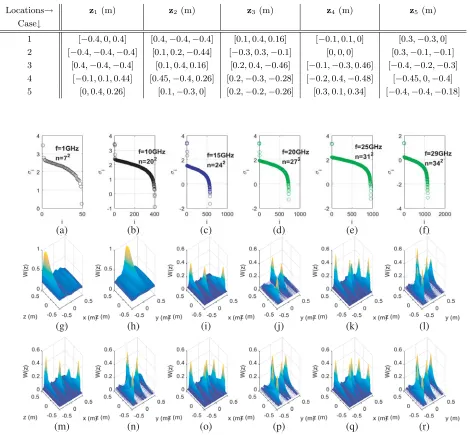
Table 1. Assumed locations of inclusions for the above seven cases (λ0 = 0.3 (m)).
Locations→ z1 (m) z2(m) z3 (m) z4 (m) z5 (m)
Case↓
1 [−0.4,0,0.4] [0.4,−0.4,−0.4] [0.1,0.4,0.16] [−0.1,0.1,0] [0.3,−0.3,0] 2 [−0.4,−0.4,−0.4] [0.1,0.2,−0.44] [−0.3,0.3,−0.1] [0,0,0] [0.3,−0.1,−0.1] 3 [0.4,−0.4,−0.4] [0.1,0.4,0.16] [0.2,0.4,−0.46] [−0.1,−0.3,0.46] [−0.4,−0.2,−0.3] 4 [−0.1,0.1,0.44] [0.45,−0.4,0.26] [0.2,−0.3,−0.28] [−0.2,0.4,−0.48] [−0.45,0,−0.4] 5 [0,0.4,0.26] [0.1,−0.3,0] [0.2,−0.2,−0.26] [0.3,0.1,0.34] [−0.4,−0.4,−0.18]
(a) (b) (c) (d) (e) (f)
(g) (h) (i) (j) (k) (l)
(m) (n) (o) (p) (q) (r)
Figure 2. The case 11. (a) to (f) The singular values ofAα in the noisy background with SNR = 5 dB,
1. For dielectric inclusions (εj =ε0 and μj =μ0).
Cases 11 to case 14 are seven examples for case 1 as Table 2. 2. For permeable inclusions (εj =ε0 and μj =μ0).
3. For lossless electromagnetic inclusions (εj =ε0 and μj =μ0).
4. For lossy electromagnetic inclusions (εj =ε0 and μj =μ0).
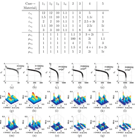
Table 2. Several examples for the cases 1–5 of Table 2.
Case→ 11 12 13 14 2 3 4 5
Material↓
εr1 12 12 10 1.1 1 3 5 4
εr2 1.5 11 10 1.1 1 5 1.1i 1
εr3 2 2 10 1.1 1 7 2.5 + 3i 3
εr4 1.1 10 10 1.1 1 4 2.5i 5i
εr5 3 3 10 1.1 1 8 4i 1
μr1 1 1 1 1 1.1 3 3 + 2i 1
μr2 1 1 1 1 100 6 2i 1.1
μr3 1 1 1 1 4 7 7i 3
μr4 1 1 1 1 1.5 4 4 +i 3 + 2i
μr5 1 1 1 1 5 2 2i 5i
(a) (b) (c) (d) (e) (f)
(g) (h) (i) (j) (k) (l)
(m) (n) (o) (p) (q) (r)
(a) (b) (c) (d) (e)
(f) (g) (h) (i)
Figure 4. The case 4. (a) Random locations of inclusions in 3D. (b) The singular values of Aα in a noise-free and a noisy background with n = 72, SNR = 5 dB, and f = 1 GHz. (c) The locations of the lossy electromagnetic inclusions in a noise-free background in x-z plane for f = 1 GHz. (d) The locations of the lossy electromagnetic inclusions in a noise-free background in y-zplane for f = 1 GHz. (e) The locations of the lossy electromagnetic inclusions in a noisy background with SNR = 5 dB inx-z plane for f = 1 GHz. (f) The locations of the lossy electromagnetic inclusions in a noisy background with SNR = 5 dB in y-zplane for f = 1 GHz. (g) The singular values of Aα in a noise-free and a noisy background withn= 242, SNR = 5 dB, andf = 15 GHz. (h) The locations of the lossy electromagnetic inclusions in a noisy background with SNR = 5 dB inx-zplane forf = 15 GHz. (i) The locations of the lossy electromagnetic inclusions in a noisy background with SNR = 5 dB in y-z plane forf = 15 GHz.
5. For some combinations of the previous cases.
The locations inclusions for different cases are assumed as in Table 1, and materials of inclusions for different examples of cases are as considered in Table 2.
By increasing the frequency to 29 GHz, we simulate case 11 and case 4, and the results are shown in Figures 2 and 3.
We have shown results of, case 11 in Figure 2, and case 4 with random locations in Figures 3 and 4.
At the end, we have investigated the proposed formulation for the extended targets. As shown in Figure 5, two separate magnetic circles with μ = 2μ0, ε = ε0 are retrieved that are placed in plane z= 0.2 m and z=−0.2 m. Each target is extended by 10 point scatterers. Two separate circles or two extended targets, one times in a noise-free and the other time in a noisy background with SNR = 5 dB, are shown in Figure 5.
Finally some cases are selected from Table 2 for simulation as in Table 3.
Description for Table 3: In all cases, the differences between singular values Aα for a noise-free background are very considerable, and all of the inclusions are restored.
(a) (b) (c) (d) (e)
(f) (g) (h) (i) (j)
Figure 5. The extended targets forn= 112 and f = 4 GHz. (a) Locations of extended targets in 3D. (b) Locations of extended targets in 2D. ( (c) The singular values ofAα in a noise-free background. (d), (e), & (f) The locations of extended targets in a noise-free background. (f) The singular values of Aα in a noisy background SNR = 5. (h), (i), & (j) The locations of extended targets in a noisy background with SNR = 5 dB.
Table 3. The results of simulation of all cases in Tables 2 and 3 are as following: (for f = 1 GHz, m= 5 (number of inclusions), and n= 72 (number of transmitting/receiving antennas).
condition→ Difference between signal signal locating of
singular values Aα subspace subspace inclusions
case↓ for SNR = 5 dB for nois-free for SNR = 5 dB for SNR = 5 dB
11 very low 5m(= 25) 1 just εj = 12
12 very low 5m(= 25) 3 justεj = [12,11,10]
13 & 14 considerable 5m(= 25) 5 all of them
2 very low 2m(= 20) 3 just μj = [100,4,5]
3 low 5m(= 25) 5 all of them
4 low 5m(= 25) 5 all of them
5 very low 19 3 electromagnetic and dielectric
the test locations coincide with the locations of the inclusions; however, for other locations, this number is a very small order of magnitude equal to or less than 0.
In case 5, we have a combination of inclusions. In this case if we consider norm(Aαd)
permeable inclusion cannot be restored. Therefore forε= [4,1,3,5i,1]ε0 andμ= [1,1.1,3,3 + 2i,5i]μ0, the second and last inclusions are not restored.
By increasing the frequency to 29 GHz, the overall locating performance is improved.
8. CONCLUSION
In this paper, a new formulation for scattering matrix using MUSIC algorithm is presented to locate dielectric, permeable, electromagnetic, lossy inclusions and combination of them in a noise-free and a noisy biaxial anisotropic background. In this work, the locations of 5 isotropic ellipsoid inclusions in a permeable anisotropic background are found. This issue is studied for five cases such as dielectric, permeable, electromagnetic, lossy electromagnetic inclusions, and combination of them. Different inclusions with small, big, and middle values of εj and μj are also investigated. In all the cases, in a noise-free background the results are good. The cases with a noisy background are investigated. The number of singular values of signal subspace ofAα for SNR = 5 dB is less than noise-free background. Also, in a noise-free background all dielectric inclusions with big or small values of εj simultaneously, but in a noisy background, the inclusions with higher values of εj, which is closer to real background, are restored.
At the end, the proposed formulation for the extended targets is investigated, and the simulation results show that this formulation is appropriate for extended targets.
Therefore, the new proposed formulation of an anisotropic permeable background for object locating predicts the locations very well in a noise-free background and almost well in a noisy background for point-like inclusions or extended. As frequency increases from 1 to 29 GHz, the results have become better.
REFERENCES
1. Nikolova, N. K, “Microwave imaging for breast cancer,”IEEE Microwave Magazine, Vol. 12, No. 7, 78–94, 2011.
2. Semnani, A., I. T. Rekanos, M. Kamyab, and M. Moghaddam, “Solving inverse scattering problems based on truncated cosine Fourier and cubic B-spline expansions,”IEEE Transactions on Antennas and Propagation, Vol. 60, No. 12, 5914–5923, 2012.
3. Shamsaddini, M., A. Tavakoli, and P. Dehkhoda, “Inverse electromagnetic scattering of a dielectric cylinder buried below a slightly rough surface using a new intelligence approach,” 23rd Iranian Conference on Electrical Engineering (ICEE), 391–396, 2015.
4. Cheney, M., “The linear sampling method and the MUSIC algorithm,”Inverse Problems, Vol. 17, No. 4, 591–595, 2001.
5. Bao, G., J. Lin, and S´e. M. Mefire, “Numerical reconstruction of electromagnetic inclusions in three dimensions,”SIAM Journal on Imaging Sciences, Vol. 7, No. 1, 558–577, 2014.
6. Chen, X. and K. Agarwal, “MUSIC algorithm for two-dimensional inverse problems with special characteristics of cylinders,” IEEE Transactions on Antennas and Propagation, Vol. 56, No. 6, 1808–1812, 2008.
7. Agarwal, K. and X. Chen, “Applicability of MUSIC-type imaging in two-dimensional electromagnetic inverse problems,” IEEE Transactions on Antennas and Propagation, Vol. 56, No. 10, 3217–3223, 2008.
8. Joh, Y. D. and W. K. Park, “Structural behavior of the MUSIC-type algorithm for imaging perfectly conducting cracks,” Progress In Electromagnetics Research, Vol. 138, 211–226, 2013.
9. Joh, Y. D., Y. M. Kwon, and W. K. Park, “MUSIC-type imaging of perfectly conducting cracks in limited-view inverse scattering problems,” Applied Mathematics and Computation, Vol. 240, 273–280, 2014.
11. Ahn, C. Y., K. Jeon, and W. K. Park, “Analysis of MUSIC-type imaging functional for single, thin electromagnetic inhomogeneity in limited-view inverse scattering problem,” Journal of Computational Physics, Vol. 291, 198–217, 2015.
12. Ciuonzo, D., G. Romano, and R. Solimene, “Performance analysis of time-reversal MUSIC,”IEEE Transactions on Signal Processing, Vol. 63, No. 10, 2650–2662, 2015.
13. Devaney, A. J., “Time reversal imaging of obscured targets from multistatic data,” IEEE Transactions on Antennas and Propagation, Vol. 53, No. 5, 1600–1610, 2005.
14. Gruber, F. K., E. A. Marengo, and A. J. Devaney, “Time-reversal imaging with multiple signal classification considering multiple scattering between the targets,” The Journal of the Acoustical Society of America, Vol. 115, No. 6, 3042–3047, 2004.
15. Marengo, E. A., F. K. Gruber, and F. Simonetti, “Time-reversal MUSIC imaging of extended targets,”IEEE Transactions on Image Processing, Vol. 16, No. 8, 1967–1984, 2007.
16. Ammari, H., E. Iakovleva, and D. Lesselier, “Two numerical methods for recovering small inclusions from the scattering amplitude at a fixed frequency,”SIAM Journal on Scientific Computing, Vol. 27, No. 1, 130–158, 2005.
17. Ammari, H., E. Iakovleva, D. Lesselier, and G. Perrusson, “MUSIC-type electromagnetic imaging of a collection of small three-dimensional inclusions,”SIAM Journal on Scientific Computing, Vol. 29, No. 2, 674–709, 2007.
18. Rodeghiero, G., M. Lambert, D. Lesselier, and P. P. Ding, “Electromagnetic MUSIC imaging and 3-D retrieval of defects in anisotropic, multi-layered composite materials,” The 9th International Conference on Computational Physics (ICCP9), A05–05, 2015.
19. Shirmehenji, F., A. Zeidaabadi Nezhad, and Z. H. Firouzeh, “Object locating in anisotropic dielectric background using MUSIC algorithm,” 2016 8th International Symposium on Telecommunications (IST), 396–400, 2016.
20. Chen, L. F., C. K. Ong, C. P. Neo, V. V. Varadan, and V. K. Varadan, Microwave Electronics: Measurement and Materials Characterization, John Wiley & Sons, 2004.
21. Liu, L., L. B. Kong, G. Q. Lin, S. Matitsine, and C. R. Deng, “Microwave permeability of ferromagnetic microwires composites/metamaterials and potential applications,” IEEE Transactions on Magnetics, Vol. 44, No. 11, 3119–3122, 2008.
22. Pozar, D. M., Microwave Engineering, John Wiley & Sons, 2009.
23. Collin, R. E.,Foundations for Microwave Engineering, John Wiley & Sons, 2007.
24. Herczy´nski, A., “Bound charges and currents,”American Journal of Physics, Vol. 81, No. 3, 202– 205, 2013.
25. Ammari, H. and H. Kang, Polarization and Moment Tensors: With Applications to Inverse Problems and Effective Medium Theory, Vol. 162, 2007.
26. Catapano, I., L. Di Donato, L. Crocco, O. M. Bucci, A. F. Morabito, T. Isernia, and R. Massa, “On quantitative microwave tomography of female breast,”Progress In Electromagnetics Research, Vol. 97, 75–93, 2009.
27. Ball, J. E., “ Low signal-to-noise ratio radar target detection using linear support vector machines (L-SVM),” 2014 IEEE Radar Conference, 1291–1294, 2014.
28. Chevalier, P., A. Ferrol, and L. Albera, “High-resolution direction finding from higher order statistics: The 2rmq-MUSIC algorithm,” IEEE Transactions on Signal Processing, Vol. 54, No. 8, 2986–2997, 2006.
29. Dobrza´nski, L. A., M. Drak, and B. Zibowicz, “Materials with specific magnetic properties,”