Fully Secure Functional Encryption with General Relations from the Decisional Linear Assumption

(1)

Fully Secure Functional Encryption with General

Relations from the Decisional Linear Assumption

∗

Tatsuaki Okamoto NTT

[email protected]

Katsuyuki Takashima Mitsubishi Electric

[email protected]

December 22, 2011

Abstract

This paper presents a fully secure functional encryption scheme for a wide class of re-lations, that are speciﬁed by non-monotone access structures combined with inner-product relations. The security is proven under a standard assumption, the decisional linear (DLIN) assumption, in the standard model. The proposed functional encryption scheme covers, as special cases, (1) key-policy, ciphertext-policy and uniﬁed-policy (of key and ciphertext poli-cies) attribute-based encryption with non-monotone access structures, and (2) (hierarchical) predicate encryption with inner-product relations and functional encryption with non-zero inner-product relations.

(2)

1 Introduction

1.1 Background

Although numerous encryption systems have been developed over several thousand years, any traditional encryption system before the 1970’s had a great restriction on the relation between a ciphertext encrypted by an encryption-key and the decryption-key such that these keys should be equivalent. The innovative notion of public-key cryptosystems in the 1970’s relaxed this restriction, where these keys diﬀer and the encryption-key can be published.

Recently, a new innovative class of encryption systems, functional encryption (FE), has been extensively studied. FE provides more sophisticated and ﬂexible relations between the keys where a secret key, sk_Ψ, is associated with a parameter, Ψ, and message m is encrypted to a ciphertext Enc(m,pk,Υ) using system public key pk along with another parameter Υ. CiphertextEnc(m,pk,Υ) can be decrypted by secretsk_Ψ if and only if a relationR(Ψ,Υ) holds. FE has various applications in the areas of access control for databases, mail services, and contents distribution [3, 8, 10, 17, 18, 23, 24, 25, 26, 28].

When R is the simplest relation or equality relation, i.e., R(Ψ,Υ) holds iﬀ Ψ = Υ, it is

identity-based encryption(IBE) [4, 5, 6, 7, 11, 13, 14, 16].

(4)

true, and T(ψ) := 0 if ψ is false (For example, T(x =v) := 1 if x =v, and T(x = v) := 0 if

x=v).

If parameter Ψ for a secret key is access structure (policy) ( ˆM ,(v₁, . . . , v_i)), it is called key-policy ABE (KP-ABE). If parameter Υ for encryption is ( ˆM ,(v₁, . . . , v_i)), it is ciphertext-policy ABE (CP-ABE).

Inner-product encryption (IPE) [18] is also a class of FE, where each parameter for en-cryption and secret key is a vector over a ﬁeld or ring (e.g., −→x := (x₁, . . . , x_n) ∈ F_qn and

− →_v _{:= (}_v

1, . . . , vn) ∈ Fqn for encryption and secret key, respectively), and R(−→v ,−→x) holds iﬀ

−

→_x _{· −}→_v _{= 0, where} −→_x _{· −}→_v _{is the inner-product of} −→_x _and −→_v_{. The inner-product relation}

repre-sents a wide class of relations including equality, conjunction and disjunction (more generally, CNF and DNF) of equality relations and polynomial relations.

There are two types of secrecy in FE, attribute-hiding and payload-hiding [18]. Roughly speaking, attribute-hiding requires that a ciphertext conceal the associated attribute as well as the plaintext, while payload-hiding only requires that a ciphertext conceal the plaintext. Attribute-hiding FE is called predicate encryption (PE) [18]. Anonymous IBE and hidden-vector encryption (HVE) [10] are a class of PE and covered by predicate IPE, or PE with inner-product relations.

Although many ABE and IPE schemes have been presented over the last several years, no adaptively-secure (or fully-secure) scheme has been proposed in the standard model except [19]. The ABE scheme in [19] supports monotone access structures with equality relations and is secure under non-standard assumptions over composite order pairing groups. The IPE scheme in [19] supports inner-product relations and is secure under a non-standard assumption, whose size depends on some parameter that is not the security parameter.

No adaptively-secure (or fully-secure) ABE (even for monotone access structures) or IPE scheme has been proposed under a standard assumption in the standard model, and no adaptively-secure (or fully-adaptively-secure) ABE scheme with non-monotone access structures has been proposed (even under non-standard assumptions) in the standard model. In addition, to the best of our knowledge, no FE scheme (even with selective security) has been presented that supports more general relations than those for ABE, i.e., access structures with equality relations, and those for IPE, i.e., inner-product relations.

1.2 Our Result

• This paper proposes an adaptively secure functional encryption (FE) scheme for a wide class of relations, that are speciﬁed by non-monotone access structures combined with inner-product relations. More precisely, either one of the parameters for encryption and a secret key is a tuple of attribute vectors and the other is a non-monotone ac-cess structure or span program ˆM := (M, ρ) along with a tuple of attribute vectors, e.g., Υ := (−→x₁, . . . ,−→x_i)∈Fn1+···+ni

q for encryption, and Ψ := ( ˆM ,(−→v1, . . . ,−→vi)∈Fqn1+···+ni)

for a secret key. The component-wise inner-product relations for attribute vector compo-nents, e.g., {−→x_t· −→v_t = 0 or not }_t_∈{₁_,...,i_}, are input to span program ˆM, and R(Ψ,Υ) holds iﬀ the truth-value vector of (T(−→x₁·−→v₁ = 0), . . . ,T(−→x_i·−→v_i = 0)) is accepted by span program ˆM. Note that in this paper (e.g., Section 6), parameter (−→x₁, . . . ,−→x_i) above is ex-pressed by Γ :={(t,−→x_t)|1≤t≤d}, where 1≤t≤dmeans thattis an element of some subset of{1, . . . , d}, and parameter ( ˆM ,(−→v₁, . . . ,−→v_i)) above is expressed by S:= (M, ρ), whereρ inS is abused asρ in ˆM combined with (−→v₁, . . . ,−→v_i) (see Deﬁnition 4),

Similarly to ABE, we propose two types of FE schemes, the KP-FE and CP-FE schemes (in Sections 6 and 7), where parameter Ψ for a secret key is access structure (policy)

(5)

In addition, we show a generalized notion of KP-FE and CP-FE, unified-policy FE (UP-FE) in Section 8, where a parameter for a secret key or encryption is a combination of access structure (policy)Sand attributes Γ, and a ciphertext can be decrypted by a secret key when the both policies for the secret key and encryption are satisfied simultaneously. (The notion of UP-ABE and the first UP-ABE scheme were proposed by Attrapadung and Imai [1].)

Since the class of relations supported by the proposed FE scheme is more general than that for ABE and IPE, the proposed FE scheme includes the following schemes as special cases:

1. The (KP, CP and UP)-ABE schemes for non-monotone access structures with equal-ity relations. Here, the underlying attribute vectors of the FE scheme,{−→x_t}_t_∈{₁_,...,d_}

and {−→v_t}_t_∈{₁_,...,d_}, are specialized to two-dimensional vectors for the equality rela-tion, e.g., −→x_t := (1, x_t) and −→v_t := (v_t,−1), where −→x_t · −→v_t = 0 iﬀ x_t = v_t (see Appendices G.1 and G.2 for KP-ABE and CP-ABE).

2. The (zero-)IPE and non-zero-IPE schemes, where a non-zero-IPE scheme is a class of FE with R(−→v ,−→x) iff −→x · −→v = 0. Here, the underlying access structure S of the FE scheme is specialized to the 1-out-of-1 secret sharing. The IPE scheme, is attribute-hiding,’ where a type of key queries are not allowed in ‘weakly-attribute-hiding’ (see the definition in [19]), while there is no such restriction in ‘fully-attribute-hiding’ ([18]). See Appendix G.3 for our (weakly-attribute-hiding) IPE scheme, which is slightly modified from a straightforward IPE-specialization of our FE scheme for improving efficiency.

3. If the underlying access structure is specialized to the d-out-of-dsecret sharing, our FE scheme can be specialized to ahierarchicalzero/non-zero-IPE scheme by adding delegation and rerandomization mechanisms. We show two hierarchical (zero-)IPE (HIPE) schemes in Appendix H, where one is payload-hiding and the other (weakly) attribute-hiding.

• The proposed FE scheme with such a wide class of relations is proven to be adaptively secure (adaptively payload-hiding against CPA) under a standard assumption, the de-cisional linear (DLIN) assumption (over prime order pairing groups), in the standard model.

Note that even for FE with the simplest relations or the equality relations, i.e., IBE, only a few IBE schemes are known to be adaptively secure under standard assumptions; the Waters IBE scheme [27] under the DBDH assumption, and the Waters IBE scheme [29] under the DBDH and DLIN assumptions.

• To prove the security, this paper elaborately combines the dual system encryption method-ology proposed by Waters [29] and the concept of dual pairing vector spaces (DPVS) proposed by Okamoto and Takashima [21, 22], in a manner similar to that in [19]. See Section 2 for the concept and actual construction of DPVS.

This paper also develops a new technique to prove the security based on the DLIN as-sumption. This provides a new methodology of employing a simple assumption deﬁned on primitive groups to prove a complicated scheme that is designed on a higher level concept, DPVS.

(6)

1 and 2), that are deﬁned on DPVS. The methodology bridges the top level assumptions and the primitive one, the DLIN assumption, in a hierarchical manner, where several levels of assumptions are constructed hierarchically. Such a modular way of proof greatly clariﬁes the logic of a complicated security proof.

• The eﬃciency of the proposed FE scheme is comparable to that of the existing ABE and IPE schemes. For example, if the proposed FE scheme is specialized to IPE, the key and ciphertext sizes of our IPE scheme (Appendix G.3) are (3n+ 2)· |G|, while they are (2n+ 3)· |G|for the IPE scheme in [19], wherenis the dimension of the attribute vectors, and |G|denotes the size of an element of prime order pairing groupG, e.g., 256 bits.

• It is easy to convert the (CPA-secure) proposed FE scheme to a CCA-secure FE scheme by employing an existing general conversion such as that by Canetti, Halevi and Katz [12] or that by Boneh and Katz [9] (using additional 7-dimensional dual spaces (Bd₊₁,B∗_d₊₁) withn_d₊₁:= 2 on the proposed FE scheme, and a strongly unforgeable one-time signature scheme or message authentication code with encapsulation). That is, we can present afully secure(adaptively payload-hiding against CCA) FE scheme for the same class of relations in thestandard modelunder the DLIN assumption as well as a strongly unforgeable one-time signature scheme or message authentication code with encapsulation (see Section 9).

1.3 Notations

When A is a random variable or distribution, y←R A denotes that y is randomly selected from

A according to its distribution. When A is a set, y ←U A denotes that y is uniformly selected from A. y := z denotes that y is set, deﬁned or substituted by z. When a is a ﬁxed value,

A(x) → a (e.g., A(x) → 1) denotes the event that machine (algorithm) A outputs aon input

x. A function f :N→Ris negligible inλ, if for every constant c >0, there exists an integern

such thatf(λ)< λ−c _{for all} _{λ > n}_.

We denote the ﬁnite ﬁeld of order q by Fq, and Fq\ {0} by F_q×. A vector symbol denotes a vector representation over F_q, e.g., −→x denotes (x₁, . . . , x_n) ∈ F_qn. For two vectors −→x = (x₁, . . . , x_n) and −→v = (v₁, . . . , v_n), −→x · −→v denotes the inner-product n_i₌₁x_iv_i. The vector

−

→_{0 is abused as the zero vector in} _F_n

q for any n. XT denotes the transpose of matrix X. I and 0 denote the × identity matrix and the × zero matrix, respectively. A bold face letter denotes an element of vector space V, e.g., x ∈ V. When b_i ∈ V (i = 1, . . . , n),

spanb₁, . . . ,b_n ⊆ V (resp. span−→x₁, . . . ,−→x_n ) denotes the subspace generated by b₁, . . . ,b_n

(resp. −→x₁, . . . ,−→x_n). For vectors −→x := (x₁, . . . , x_N),−→y := (y₁, . . . , y_N) ∈ F_qN and bases B := (b₁, . . . ,b_N),B∗:= (b∗₁, . . . ,b∗_N), (→−x)_B (= (x₁, . . . , x_N)_B) denotes linear combinationN_i₌₁x_ib_i, and (−→y)_B∗ (= (y₁, . . . , y_N)_B∗) denotes N_i₌₁y_ib∗_i. For a format of attribute vectors −→n := (d;n₁, . . . , n_d) that indicates dimensions of vector spaces,−→e_t,j denotes the canonical basis vector

(

j−1

0· · ·0,1, nt−j

0· · ·0)∈Fnt

q fort= 1, . . . , d andj = 1, . . . , nt.

2 Dual Pairing Vector Spaces by Direct Product of Symmetric

Pairing Groups

(7)

polynomial-time computable nondegenerate bilinear pairing e:G×G→G_T i.e.,e(sG, tG) =e(G, G)st and

e(G, G)= 1.

Let Gbpg be an algorithm that takes input 1λ and outputs a description of bilinear pairing

groups (q,G,G_T, G, e) with security parameterλ.

In this paper, we concentrate on the symmetric version of dual pairing vector spaces [21, 22] constructed using symmetric bilinear pairing groups given in Deﬁnition 1.

Deﬁnition 2 “Dual pairing vector spaces (DPVS)” (q,V,G_T,A, e) by a direct product of sym-metric pairing groups (q,G,G_T, G, e) are a tuple of prime q, N-dimensional vector space V:=

N

G× · · · ×Gover F_q, cyclic groupG_T of orderq, canonical basisA:= (a₁, . . . ,a_N) of V, where

a_i := (

i−1

0, . . . ,0, G, N−i

0, . . . ,0), and pairing e:V×V→G_T.

The pairing is deﬁned by e(x,y) := N_i₌₁e(G_i, H_i) ∈ G_T where x := (G₁, . . . , G_N) ∈ V

and y := (H₁, . . . , H_N) ∈ V. This is nondegenerate bilinear i.e., e(sx, ty) = e(x,y)st and if

e(x,y) = 1 for all y∈V, then x=0. For alli and j, e(a_i,a_j) =e(G, G)δi,j _where _δ

i,j = 1 if i=j, and 0 otherwise, ande(G, G)= 1∈G_T.

DPVS also has linear transformations φ_i,j onVs.t.φ_i,j(a_j) =a_i andφ_i,j(a_k) =0 ifk=j,

which can be easily achieved by φ_i,j(x) := (

i−1

0, . . . ,0, G_j, N−i

0, . . . ,0) where x:= (G₁, . . . , G_N). We call φ_i,j “distortion maps”.

DPVS generation algorithmGdpvs takes input1λ (λ∈N) andN ∈N, and outputs a

descrip-tion of param_V := (q,V,G_T,A, e) with security parameter λ and N-dimensional V. It can be constructed using Gbpg.

For the asymmetric version of DPVS, (q,V,V∗,G_T,A,A∗, e), see Appendix A.2. The above symmetric version is obtained by identifyingV=V∗ and A=A∗ in the asymmetric version.

We describe random dual orthonormal basis generator Gob below, which is used as a

sub-routine in the proposed FE scheme.

Gob(1λ,−→n := (d;n1, . . . , nd)) :paramG := (q,G,GT, G, e)

R

← Gbpg(1λ), ψ U ←F×

q , N₀ := 5, N_t:= 3n_t+ 1 for t= 1, . . . , d,

fort= 0, . . . , d,

param_V_t := (q,Vt,GT,At, e) :=Gdpvs(1λ, Nt,paramG),

X_t:=

⎛ ⎜ ⎝

− →_χ

t,1

.. .

− →_χ

t,Nt

⎞ ⎟

⎠:= (χ_t,i,j)_i,j ←U GL(N_t,F_q),

⎛ ⎜ ⎝

− →

ϑ_t,₁

.. .

− →

ϑ_t,N_t

⎞ ⎟

⎠:= (ϑ_t,i,j)_i,j :=ψ·(X_tT)−1,

b_t,i := (−→χ_t,i)_A_t =Nt

j=1χt,i,jat,j fori= 1, . . . , Nt, Bt:= (bt,1, . . . ,bt,Nt),

b∗_t,i := (−→ϑ_t,i)_A_t =Nt

j=1ϑt,i,jat,j fori= 1, . . . , Nt, B∗t := (b∗t,1, . . . ,b∗t,Nt),

g_T :=e(G, G)ψ, param−→_n := ({param_V_t}_t₌₀_,...,d, g_T),

return (param−→_n,{Bt,B∗_t}_t₌₀_,...,d).

(8)

3 Functional Encryption with General Relations

3.1 Span Programs and Non-Monotone Access Structures

Deﬁnition 3 (Span Programs [2]) Let {p₁, . . . , p_n} be a set of variables. A span program over F_q is a labeled matrixMˆ := (M, ρ) where M is a (×r) matrix overF_q and ρis a labeling of the rows ofM by literals from{p₁, . . . , p_n,¬p₁, . . . ,¬p_n}(every row is labeled by one literal), i.e.,ρ:{1, . . . , } → {p₁, . . . , p_n,¬p₁, . . . ,¬p_n}.

A span program accepts or rejects an input by the following criterion. For every input sequenceδ ∈ {0,1}n deﬁne the submatrix M_δ of M consisting of those rows whose labels are set to 1 by the input δ, i.e., either rows labeled by some p_i such thatδ_i = 1 or rows labeled by some ¬p_i such that δ_i = 0. (i.e., γ :{1, . . . , } → {0,1} is deﬁned by γ(j) = 1 if [ρ(j) =p_i]∧[δ_i = 1]

or [ρ(j) =¬p_i]∧[δ_i= 0], and γ(j) = 0otherwise. M_δ := (M_j)_γ₍_j₎₌₁, where M_j is thej-th row of M.)

The span programMˆ acceptsδ if and only if−→1 ∈spanM_δ , i.e., some linear combination of the rows ofM_δgives the all one vector−→1. (The row vector has the value 1 in each coordinate.) A span program computes a Boolean functionf if it accepts exactly those inputsδ where f(δ) = 1. A span program is called monotone if the labels of the rows are only the positive literals

{p₁, . . . , p_n}. Monotone span programs compute monotone functions. (So, a span program in

general is “non”-monotone.)

We assume that the matrix M satisﬁes the condition: M_i=−→0 fori= 1, . . . , .

We now introduce a non-monotone access structure with evaluating map γ by using the inner-product of attribute vectors, that is employed in the proposed functional encryption schemes.

Deﬁnition 4 (Inner-Products of Attribute Vectors and Access Structures) U_t(t= 1,

. . . , d and U_t ⊂ {0,1}∗) is a sub-universe, a set of attributes, each of which is expressed by

a pair of sub-universe id and n_t-dimensional vector, i.e., (t,−→v), where t ∈ {1, . . . , d} and −

→_v _∈_Fnt

q \ {−

→

0}.

We now deﬁne such an attribute to be a variable p of a span program Mˆ := (M, ρ), i.e., p := (t,−→v). An access structure S is span program Mˆ := (M, ρ) along with variables

p := (t,−→v), p := (t,−→v), . . ., i.e., S := (M, ρ) such that ρ : {1, . . . , } → {(t,−→v),(t,−→v), . . ., ¬(t,−→v),¬(t,−→v), . . .}.

Let Γbe a set of attributes, i.e., Γ :={(t,−→x_t)| −→x_t∈Fnt

q \{−→0},1≤t≤d}, where1≤t≤d

means that tis an element of some subset of {1, . . . , d}.

When Γ is given to access structure S, map γ :{1, . . . , } → {0,1} for span program Mˆ := (M, ρ) is deﬁned as follows: For i = 1, . . . , , set γ(i) = 1 if [ρ(i) = (t,−→v_i)] ∧[(t,−→x_t) ∈ Γ]

∧[−→v_i· −→x_t= 0] or [ρ(i) =¬(t,−→v_i)] ∧[(t,−→x_t)∈Γ]∧[−→v_i· −→x_t= 0]. Set γ(i) = 0 otherwise. Access structure S:= (M, ρ) accepts Γ iﬀ −→1 ∈span(M_i)_γ₍_i₎₌₁ .

We now construct a secret-sharing scheme for a non-monotone access structure or span program.

Deﬁnition 5 A secret-sharing scheme for span program Mˆ := (M, ρ) is:

1. Let M be ×r matrix. Let column vector −→fT := (f₁, . . . , f_r)T ←U F_qr. Then, s₀ :=

− →

(9)

2. If span program Mˆ := (M, ρ) accept δ, or access structure S := (M, ρ) accepts Γ, i.e., −

→₁ _∈ _span₍_M

i)γ(i)=1 with γ : {1, . . . , } → {0,1}, then there exist constants {αi ∈ Fq | i∈I} such that I ⊆ {i ∈ {1, . . . , } | γ(i) = 1} and _i_∈_Iα_is_i =s₀. Furthermore, these constants {α_i} can be computed in time polynomial in the size of matrixM.

3.2 Key-Policy Functional Encryption with General Relations

Deﬁnition 6 (Key-Policy Functional Encryption : KP-FE) A key-policy functional en-cryption scheme consists of four algorithms.

Setup This is a randomized algorithm that takes as input security parameter and format −→n := (d;n₁, . . . , n_d) of attributes. It outputs public parameters pk and master secret key sk.

KeyGen This is a randomized algorithm that takes as input access structureS:= (M, ρ),pk and

sk. It outputs a decryption key sk_S.

Enc This is a randomized algorithm that takes as input message m, a set of attributes, Γ :=

{(t,−→x_t)|−→x_t ∈Fnt

q \ {−

→

0},1 ≤ t ≤d}, and public parameters pk. It outputs a ciphertext

ct_Γ.

Dec This takes as input ciphertextct_Γ that was encrypted under a set of attributesΓ, decryption key sk_S for access structure S, and public parameters pk. It outputs either plaintextm or the distinguished symbol ⊥.

A KP-FE scheme should have the following correctness property: for all (pk,sk)←R Setup(1λ,

−

→_n_{), all access structures} _S_{, all decryption keys} _sk

S ←R KeyGen(pk,sk,S), all messages m, all

attribute sets Γ, all ciphertexts ct_Γ ←R Enc(pk, m,Γ), it holds that m =Dec(pk,sk_S,ct_Γ) with overwhelming probability, ifS accepts Γ.

Deﬁnition 7 The model for proving the adaptively payload-hiding security of KP-FE under chosen plaintext attack is:

Setup The challenger runs the setup algorithm, (pk,sk) ←R Setup(1λ, −→n), and gives public parameters pk to the adversary.

Phase 1 The adversary is allowed to adaptively issue a polynomial number of queries, S, to the challenger or oracle KeyGen(pk,sk,·) for private keys, sk_S associated with S.

Challenge The adversary submits two messagesm(0), m(1) and a set of attributes,Γ, provided that no S queried to the challenger in Phase 1 accepts Γ. The challenger ﬂips a coin

b← {U 0,1}, and computes ct(_Γb)←R Enc(pk, m(b),Γ). It gives ct(_Γb) to the adversary.

Phase 2 The adversary is allowed to adaptively issue a polynomial number of queries, S, to the challenger or oracleKeyGen(pk,sk,·) for private keys,sk_S associated with S, provided thatS does not accept Γ.

Guess The adversary outputs a guess b of b.

The advantage of adversary A in the above game is deﬁned as AdvKP_A -FE,PH(λ) := Pr[b =

(10)

We note that the model can easily be extended to handle chosen-ciphertext attacks (CCA) by allowing for decryption queries in Phases 1 and 2. The advantage of adversary A in the CCA game is deﬁned as AdvKP_A -FE,CCA-PH(λ) := Pr[b=b]−1/2 for any security parameterλ.

3.3 Ciphertext-Policy Functional Encryption with General Relations

Deﬁnition 8 (Ciphertext-Policy Functional Encryption : CP-FE) A ciphertext-policy functional encryption scheme consists of four algorithms.

Setup This is a randomized algorithm that takes as input security parameter and format −→n := (d;n₁, . . . , n_d) of attributes. It outputs the public parameters pk and a master key sk.

KeyGen This is a randomized algorithm that takes as input a set of attributes,Γ :={(t,−→x_t)|−→x_t

∈Fnt

q ,1≤t≤d}, pk and sk. It outputs a decryption key.

Enc This is a randomized algorithm that takes as input messagem, access structureS:= (M, ρ), and the public parameters pk. It outputs the ciphertext.

Dec This takes as input the ciphertext that was encrypted under access structureS, the decryp-tion key for a set of attributesΓ, and the public parameters pk. It outputs either plaintext

m or the distinguished symbol ⊥.

A CP-FE scheme should have the following correctness property: for all (pk,sk)←R Setup(1λ,

−

→_n_{), all attribute sets Γ, all decryption keys} _sk

Γ←R KeyGen(pk,sk,Γ), all messagesm, all access structures S, all ciphertexts ct_S ←R Enc(pk, m,S), it holds that m = Dec(pk,sk_Γ,ct_S) with overwhelming probability, ifS accepts Γ.

Deﬁnition 9 The model for proving the adaptively payload-hiding security of CP-FE under chosen plaintext attack is:

Setup The challenger runs the setup algorithm, (pk,sk) ←R Setup(1λ_,−→_n₎_{, and gives the public}

parameters pk to the adversary.

Phase 1 The adversary is allowed to issue a polynomial number of queries, Γ, to the challenger or oracle KeyGen(pk,sk,·) for private keys, sk_Γ associated with Γ.

Challenge The adversary submits two messages m(0), m(1) and an access structure, S := (M, ρ), provided that the S does not accept any Γ sent to the challenger in Phase 1.

The challenger ﬂips a random coin b← {U 0,1}, and computes ct_S(b)←R Enc(pk, m(b),S). It gives ct(_Sb) to the adversary.

Phase 2 The adversary is allowed to issue a polynomial number of queries, Γ, to the challenger or oracleKeyGen(pk,sk,·) for private keys, sk_Γ associated withΓ, provided thatS does not accept Γ.

Guess The adversary outputs a guess b of b.

The advantage of an adversaryA in the above game is deﬁned asAdvCP_A -FE,PH(λ) := Pr[b =

b]−1/2 for any security parameter λ. A CP-FE scheme is adaptively payload-hiding secure if all polynomial time adversaries have at most a negligible advantage in the above game.

(11)

3.4 Uniﬁed-Policy Functional Encryption with General Relations

Definition 10 (Unified-Policy Functional Encryption : UP-FE) A unified-policy func-tional encryption scheme consists of four algorithms.

Setup This is a randomized algorithm that takes as input security parameter and format −→n := ((dKP;nKP₁ , . . . , nKP_dKP),(dCP;nCP1 , . . . , nCP_dCP)) of attributes. It outputs public parameters pk

and master secret key sk.

KeyGen This is a randomized algorithm that takes as input access structureSKP := (MKP, ρKP), a set of attributes, ΓCP := {(t,−→x_tCP)|−→xCP_t ∈ FnCPt

q \ {−→0},1 ≤ t ≤ dCP}, pk and sk. It

outputs a decryption keysk₍_SKP_,_ΓCP₎.

Enc This is a randomized algorithm that takes as input message m, a set of attributes, ΓKP :=

{(t,−→xKP_t )|−→xKP_t ∈ FnKPt

q \ {−→0},1 ≤ t ≤ dKP}, access structure SCP := (MCP, ρCP), and

public parameters pk. It outputs a ciphertext ct_(ΓKP_,_SCP₎.

Dec This takes as input a ciphertext ct_(ΓKP_,_SCP₎ that was encrypted under a set of attributes

and access structure, (ΓKP,SCP), decryption key sk₍_SKP_,_ΓCP₎ for access structure and a set

of attributes, (SKP,ΓCP), and public parameters pk. It outputs either plaintext m or the distinguished symbol ⊥.

A UP-FE scheme should have the following correctness property: for all (pk,sk)←R Setup(1λ_,

−

→_n_{), all access structures}_SKP_{, all attribute sets Γ}CP_{, all decryption keys}_sk

(SKP_,_ΓCP₎

R

←KeyGen(pk,

sk,SKP,ΓCP), all messages m, all attribute sets ΓKP, all access structures SCP, all ciphertexts

ct_(ΓKP_,_SCP₎

R

← Enc(pk, m,ΓKP,SCP), it holds that m = Dec(pk,sk₍_SKP_,_ΓCP₎,ct_(ΓKP_,_SCP₎) with over-whelming probability, if SKP _{accepts Γ}KP _and _SCP _{accepts Γ}CP_.

The adaptively payload-hiding security of UP-FE under chosen plaintext attack (and chosen ciphertext attack) are deﬁned similarly as those of KP-FE and CP-FE. (See Deﬁnition 7 and 9.)

4 Decisional Linear (DLIN) Assumption

Deﬁnition 11 (DLIN: Decisional Linear Assumption) The DLIN problem is to guessβ ∈

{0,1}, given (param_G, G, ξG, κG, δξG, σκG, Y_β)← GR DLIN

β (1λ), where

GDLIN

β (1λ) :paramG := (q,G,GT, G, e)

R

← Gbpg(1λ),

κ, δ, ξ, σ←UF_q, Y₀ := (δ+σ)G, Y₁ ←UG,

return (param_G, G, ξG, κG, δξG, σκG, Y_β),

for β ← {U 0,1}. For a probabilistic machine E, we deﬁne the advantage of E for the DLIN problem as:

AdvDLIN_E (λ) := Pr

E(1λ, )→1 ←GR ₀DLIN(1λ)

−Pr

E(1λ, )→1 ←GR ₁DLIN(1λ).

The DLIN assumption is: For any probabilistic polynomial-time adversary E, the advantage

(12)

5 Lemmas for the Proofs of Main Theorems

We will show three lemmas for the proof of Theorems 1 and 2.

Deﬁnition 12 (Problem 1) Problem 1 is to guessβ, given(param−→_n,B₀,B∗₀,e_β,₀,{B_t,B∗_t,e_β,t,₁,

e_t,i}_t₌₁_,...,d_;_i₌₂_,...,n_t)← GR _βP1(1λ,−→n), where

GP1

β (1λ,−→n) : (param−→n,{Bt,B∗t}t=0,...,d)

R

← Gob(1λ,−→n),

B∗₀:= (b∗₀_,₁,b∗₀_,₃, ..,b∗₀_,₅), B∗_t := (b∗_t,₁, ..,b∗_t,n_t,b∗_t,₂_n_t₊₁, ..,b∗_t,₃_n_t₊₁) fort= 1, .., d,

ω, z₀, γ₀ ←UF_q, e₀_,₀ := (ω,0,0,0, γ₀)_B₀, e₁_,₀ := (ω, z₀,0,0, γ₀)_B₀,

fort= 1, . . . , d;

− →_e

t,1 := (1,0nt−1)∈Fqnt, −→zt

U ←Fnt

q , γt

U ←Fq, nt

nt nt 1

e₀_,t,₁ := ( ω−→e_t,₁, 0nt_, ₀nt_, _γ

t )Bt,

e₁_,t,₁ := ( ω−→e_t,₁, −→z_t, 0nt_, _γ

t )Bt,

e_t,i :=ωb_t,i fori= 2, . . . , n_t,

return (param−→_n,B₀,B₀∗,e_β,₀,{B_t,B∗_t,e_β,t,₁,e_t,i}_t₌₁_,...,d_;_i₌₂_,...,n_t),

for β ← {U 0,1}. For a probabilistic machineB, we deﬁne the advantage ofB as the quantity

AdvP1_B (λ) :=Pr

B(1λ, )→1←GR ₀P1(1λ,−→n)

−Pr

B(1λ, )→1←GR ₁P1(1λ,−→n).

Lemma 1 For any adversary B, there exist probabilistic machines E, whose running times are essentially the same as that of B, such that for any security parameter λ, AdvP1_B (λ) ≤

AdvDLIN_E (λ) + (d+ 6)/q.

Deﬁnition 13 (Problem 2) Problem 2 is to guessβ, given (param−→_n,B₀,B∗₀,h∗_β,₀,e₀,{B_t,B∗_t,

h∗_β,t,i,e_t,i}_t₌₁_,...,d_;_i₌₁_,...,n_t)← GR P2

β (1λ,−→n), where

GP2

β (1λ,−→n) : (param−→n,{Bt,B∗t}t=0,...,d)

R

← Gob(1λ,−→n),

B0:= (b₀_,₁,b₀_,₃, ..,b₀_,₅), Bt := (b_t,₁, ..,b_t,n_t,b_t,₂_n_t₊₁, ..,b_t,₃_n_t₊₁) fort= 1, .., d, δ, δ₀, ω ←UFq, τ, u₀ ←UF_q×, z₀:=u−₀1,

⎛ ⎜ ⎝ − →_z t,1 .. . − →_z t,nt ⎞ ⎟

⎠:=Z_t←U GL(n_t,Fq),

⎛ ⎜ ⎝ − →_u t,1 .. . − →_u t,nt ⎞ ⎟

⎠:= (Z_t−1)T for t= 1, .., d,

h∗₀_,₀ := (δ,0,0, δ₀,0)_B∗

0, h∗1,0:= (δ, u0,0, δ0,0)B∗0, e0:= (ω, τ z0,0,0,0)B0,

fort= 1, . . . , d; i= 1, . . . , n_t;

− →_e

t,i:= (0i−1,1,0nt−i)∈Fqnt,

− →

δ_t,i ←UFnt

q , nt

nt nt 1

h∗₀_,t,i:= ( δ−→e_t,i, 0nt_, −→_δ

t,i, 0 )B∗t

h∗₁_,t,i:= ( δ−→e_t,i, →−u_t,i, −→δ_t,i, 0 )_B∗

t

e_t,i := ( ω−→e_t,i, τ−→z_t,i, 0nt_, ₀ ₎

Bt,

(13)

for β← {U 0,1}. For a probabilistic adversaryB, the advantage ofB for Problem 2,AdvP2_B (λ), is similarly deﬁned as in Deﬁnition 12.

Lemma 2 For any adversary B, there exists a probabilistic machine E, whose running time is essentially the same as that of B, such that for any security parameter λ, AdvP2_B (λ) ≤

AdvDLIN_E (λ) + 5/q.

Lemma 3 Forp∈F_q, letC_p:={(−→x ,−→v)|−→x·−→v =p} ⊂V×V∗ whereV isn-dimensional vector spaceFn

q, andV∗ its dual. For all(−→x ,→−v)∈Cp, for all(−→r ,→−w)∈Cp,Pr [−→x U =−→r ∧ −→v Z=−→w]

= Pr [−→x Z=−→r ∧ −→v U =−→w] = 1 C_p, where Z ←UGL(n,F_q), U := (Z−1)T.

6 KP-FE Scheme

6.1 Construction

We deﬁne function ρ:{1, . . . , } → {1, . . . , d} by ρ(i) := t if ρ(i) = (t,−→v) or ρ(i) = ¬(t,−→v), where ρ is given in access structureS:= (M, ρ). In the proposed scheme, we assume that ρis injective for S:= (M, ρ) with decryption key sk_S. We will show how to relax the restriction in Appendix F.

In the description of the scheme, we assume that input vector, −→x_t := (x_t,₁, . . . , x_t,n_t), is normalized such that x_t,₁ := 1. (If −→x_t is not normalized, change it to a normalized one by (1/x_t,₁)· −→x_t, assuming that x_t,₁ is non-zero).

Random dual basis generator Gob(1λ,−→n) is deﬁned at the end of Section 2. We refer to

Section 1.3 for notations on DPVS.

Setup(1λ, −→n := (d;n₁, . . . , n_d)) : (param−→_n,{B_t,B∗_t}_t₌₀_,...,d)← GR ob(1λ,−→n),

B0 := (b0,1,b0,3,b0,5), Bt:= (bt,1, ..,bt,nt,bt,3nt+1) fort= 1, .., d,

B∗₀ := (b∗₀_,₁,b∗₀_,₃,b∗₀_,₄), B∗_t := (b∗_t,₁, ..,b∗_t,n_t,b∗_t,₂_n_t₊₁, ..,b∗_t,₃_n_t) fort= 1, .., d,

pk:= (1λ,param−→_n,{B_t}_t₌₀_,...,d), sk:={B∗_t}_t₌₀_,...,d,

return pk, sk.

KeyGen(pk, sk, S:= (M, ρ)) :

− →

f ←UF_qr, −→sT := (s₁, . . . , s)T:=M·−→fT, s₀ :=−→1 ·−→fT, η₀ ←U F_q,

k∗₀ := (−s₀, 0, 1, η₀, 0)_B∗

0,

fori= 1, . . . , ,

if ρ(i) = (t,−→v_i:= (v_i,₁, . . . , v_i,n_t)∈Fnt

q \ {−→0}), θi

U

←Fq, −→ηi

U ←Fnt

q , nt

nt nt 1

k∗_i := ( s_i−→e_t,₁+θ_i−→v_i, 0nt_, −→_η

i, 0 )B∗t,

if ρ(i) =¬(t,−→v_i), −→η_i ←U Fnt

q , nt

nt nt 1

k∗_i := ( s_i−→v_i, 0nt_, −→_η

i, 0 )B∗t,

return sk_S:= (S,k₀∗,k∗₁, . . . ,k∗).

Enc(pk, m, Γ :={(t,−→x_t:= (x_t,₁, .., x_t,n_t)∈Fnt

q \ {−→0})|1≤t≤d, xt,1 := 1}) : ω, ϕ₀, ϕ_t, ζ ←U Fq for (t,−→x_t)∈Γ,

(14)

nt

nt nt 1

c_t:= ( ω−→x_t, 0nt_, ₀nt_, _ϕ

t )Bt for (t,−→xt)∈Γ,

c_d₊₁:=g_Tζm, ct_Γ:= (Γ,c₀,{c_t}₍_t,−→_x_t₎_∈_Γ, c_d₊₁),

return ct_Γ.

Dec(pk, sk_S:= (S,k₀∗,k∗₁, . . . ,k∗), ct_Γ:= (Γ,c₀,{c_t}₍_t,−→_x_t₎_∈_Γ, c_d₊₁)) :

If S:= (M, ρ) accepts Γ :={(t,−→x_t)}, then computeI and {α_i}_i_∈_I such that

− →

1 =_i_∈_Iα_iM_i, whereM_i is thei-th row ofM, and

I ⊆ {i∈ {1, . . . , } | [ρ(i) = (t,−→v_i) ∧ (t,−→x_t)∈Γ ∧ −→v_i· −→x_t= 0]

∨ [ρ(i) =¬(t,−→v_i) ∧ (t,→−x_t)∈Γ ∧ −→v_i· −→x_t= 0] },

K :=e(c₀,k₀∗)

i∈I∧ ρ(i)=(t,−→vi)

e(c_t,k∗_i)αi

i∈I ∧ ρ(i)=¬(t,−→vi)

e(c_t,k∗_i)αi/(−→vi·−→xt)_,

return m :=c_d₊₁/K.

[Correctness] IfS:= (M, ρ) accepts Γ :={(t,−→x_t)},

e(c₀,k∗₀)_i_∈_I _∧ _ρ₍_i₎₌₍_t,−→_v_i₎e(c_t,k∗_i)αi·

i∈I ∧ ρ(i)=¬(t,−→vi)e(ct,k

∗

i)αi/(

− →_v_i_·−→_x_t₎

=g_T−δs0+ζ_i_∈_I _∧ _ρ₍_i₎₌₍_t,−→_v_i₎gδαisi

T

i∈I ∧ ρ(i)=¬(t,−→vi)g

δαisi(−→vi·−→xt)/(−→vi·−→xt)

T

=gδ(−s0+

P

i∈Iαisi)+ζ

T =gTζ.

6.2 Security

Theorem 1 The proposed KP-FE scheme is adaptively payload-hiding against chosen plaintext attacks under the DLIN assumption.

For any adversaryA, there exist probabilistic machinesE₁,E₂+, andE₂, whose running times are essentially the same as that of A, such that for any security parameter λ,

AdvKP_A -FE,PH(λ)≤AdvDLIN_E₁ (λ) +

ν−1

h=0

AdvDLIN_E+ 2,h

(λ) +AdvDLIN_E₂

,h+1(λ)

+,

where E₂+_,h(·) := E₂+(h,·),E₂_,h₊₁(·) := E₂(h,·) (h = 0, . . . , ν −1), ν is the maximum number of A’s key queries and := (2dν+ 16ν+d+ 7)/q.

Proof Outline of Theorem 1: At the top level of strategy of the security proof, we follow the dual system encryption methodology proposed by Waters [29]. In the methodology, ciphertexts and secret keys have two forms, normal and semi-functional. In the proof herein, we also introduce another form calledpre-semi-functional. The real system uses only normal ciphertexts and normal secret keys, and semi-functional/pre-semi-functional ciphertexts and keys are used only in a sequence of security games for the security proof.

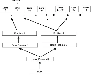
To prove this theorem, we employ Game 0 (original adaptive-security game) through Game 3. In Game 1, the challenge ciphertext is changed to semi-functional. When at most ν secret key queries are issued by an adversary, there are 2ν game changes from Game 1 (Game 2-0), Game 2-0+, Game 2-1 through Game 2-(ν −1)+ and Game 2-ν. In Game 2-h, the ﬁrst h

keys are semi-functional while the remaining keys are normal, and the challenge ciphertext is semi-functional. In Game 2-h+, the ﬁrst h keys are semi-functional and the (h+ 1)-th key is

(15)

For sk_S := (S,k₀∗,k₁∗, . . . ,k∗) and ct_Γ := (Γ,c₀, {c_t}₍_t,−→_x_t₎_∈_Γ, c_d₊₁), we focus on −→k∗_S := (k₀∗,k∗₁, . . . ,k∗) and−→c_Γ := (c₀,{c_t}₍_t,−→_x_t₎_∈_Γ), and ignore the other part of sk_S andct_Γ(and call them secret key and ciphertext, respectively) in this proof outline. In addition, we ignore a negligible factor in the (informal) descriptions of this proof outline. For example, we say “A is bounded by B” whenA≤B+(λ) where(λ) is negligible in security parameterλ.

A normal secret key, −→k∗_Snorm (with access structure S), is the correct form of the secret key of the proposed FE scheme, and is expressed by Eq. (1). Similarly, a normal ciphertext (with attribute set Γ), −→cnorm_Γ , is expressed by Eq. (2). A semi-functional secret key, −→k∗_Ssemi, is expressed by Eq. (8), and a semi-functional ciphertext, −→csemi_Γ , is expressed by Eqs. (3)-(5). A pre-semi-functional secret key, −→k∗_Spre-semi, andpre-semi-functional ciphertext,−→cpre_Γ -semi, are expressed by Eq. (6) and Eqs. (3), (7) and (5), respectively.

To prove that the advantage gap between Games 0 and 1 is bounded by the advantage of Problem 1 (to guess β ∈ {0,1}), we construct a simulator of the challenger of Game 0 (or 1) (against an adversary A) by using an instance with β ← {U 0,1} of Problem 1. We then show that the distribution of the secret keys and challenge ciphertext replied by the simulator is equivalent to those of Game 0 when β = 0 and those of Game 1 when β = 1. That is, the advantage of Problem 1 is equivalent to the advantage gap between Games 0 and 1 (Lemma 4). The advantage of Problem 1 is proven to be equivalent to that of the DLIN assumption (Lemma 1).

The advantage gap between Games 2-h and 2-h+ is similarly shown to be bounded by the advantage of Problem 2 (i.e., advantage of the DLIN assumption) (Lemmas 5 and 2). Here, we introduce special forms of pre-semi-functional keys and ciphertexts, −→k∗_Sspec.pre-semi

and −→cspec_Γ .pre-semi, respectively, such that they are equivalent to pre-semi-functional keys and ciphertexts, −→k∗_Spre-semi and−→cpre_Γ -semi, respectively, except thatw₀r₀ =a₀:=_kr₌₁g_k and r₀ ←U Fq (note that r0, w0

U

← Fq for −→k_S∗ pre-semi and −→cpre_Γ -semi). These forms of keys and ciphertexts,

− →

k∗_Sspec.pre-semiand→−cspec_Γ .pre-semi, are simulated using Problem 2 withβ = 1. From the deﬁnition of these forms, −→k∗_Sspec.pre-semi can decrypt −→cspec_Γ .pre-semi for any Γ when S accepts Γ, i.e., it is hard for simulator B+₂ to tell (−→k∗_Sspec.pre-semi, →−cspec_Γ .pre-semi) for Game 2-h+ from (−→k∗ norm

S ,

− →_csemi

Γ ) for Game 2-h under the assumption of Problem 2. On the other hand, a0(= w0r0) is independently distributed from the other variables when S does not accept Γ (shown in Proof of Claim 1 by using Lemma 3). That is, the joint distribution of −→k∗_Spre-semi and −→cpre_Γ -semi is equivalent to that of −→k∗_Sspec.pre-semi and −→cspec_Γ .pre-semi, when S does not accept Γ (i.e., B+₂’s simulation using Problem 2 with β = 1 is the same distribution as that of Game 2-h+ from the adversary’s view). In other words, w₀ and r₀ in −→k_S∗ spec.pre-semi and −→cspec_Γ .pre-semi (given by

B+₂’s simulation using Problem 2 with β = 1) are correlated for the case that S accepts Γ or for simulatorB₂+’s view, but adversaryAcannot notice the correlation sinceA’s queries should satisfy the condition that Sdoes not accept Γ.

The advantage gap between Games 2-h+ and 2-(h+ 1) is similarly shown to be bounded by the advantage of Problem 2, i.e., advantage of the DLIN assumption (Lemmas 6 and 2).

Finally we show that Game 2-ν can be conceptually changed to Game 3 (Lemma 7).

Proof of Theorem 1 : To prove Theorem 1, we consider the following (2ν+ 3) games. In Game 0, a part framed by a box indicates coeﬃcients to be changed in a subsequent game. In the other games, a part framed by a box indicates coeﬃcients which were changed in a game from the previous game.

(16)

M is:

k₀∗:= (−s₀, 0, 1, η₀, 0)_B∗

0,

fori= 1, . . . , ,

if ρ(i) = (t,−→v_i), k∗_i := (s_i→−e_t,₁+θ_i−→v_i, 0nt _, −→_η

i, 0)B∗

t,

if ρ(i) =¬(t,−→v_i), k_i∗:= (s_i−→v_i, 0nt _, −→_η

i, 0)B∗t,

⎫ ⎪ ⎪ ⎪ ⎪ ⎪ ⎬ ⎪ ⎪ ⎪ ⎪ ⎪ ⎭ (1)

where −→f ←U F_qr,−→sT:= (s₁, . . . , s)T :=M·−→fT, s₀ :=−→1 ·−→f T, θ_i, η₀ ←UFq,−→η_i ←U Fnt

q ,−→et,1 =

(1,0, . . . ,0) ∈ Fnt

q , and −→vi ∈ Fqnt \ {−→0}. The challenge ciphertext for challenge plaintexts

(m(0), m(1)) and Γ :={(t,−→x_t)|1≤t≤d} is:

c₀ := (δ, 0, ζ , 0, ϕ₀)_B₀,

c_t:= (δ−→x_t, 0nt _, ₀nt_{, ϕ}

t)Bt for (t,−→xt)∈Γ,

c_d₊₁ :=gζ_Tm(b),

⎫ ⎪ ⎪ ⎬ ⎪ ⎪ ⎭ (2)

whereb← {U 0,1};δ, ζ, ϕ₀, ϕ_t←U F_q, and −→x_t∈Fnt

q \ {−→0}.

Game 1 : Same as Game 0 except that the challenge ciphertext is:

c₀:= (δ, r₀ , ζ, 0, ϕ₀)_B₀, (3)

c_t:= (δ−→x_t, −→r_t , 0nt_{, ϕ}

t)Bt for (t,−→xt)∈Γ, (4)

c_d₊₁:=g_Tζm(b), (5)

wherer₀←UFq,−→r_t←U Fnt

q , and all the other variables are generated as in Game 0.

Game 2-h+(h= 0, . . . , ν−1) : Game 2-0 is Game 1. Game 2-h+ is the same as Game 2-h

except the reply to the (h+ 1)-th key query forS:= (M, ρ) with ×r matrixM, and c_t of the challenge ciphertext are:

k₀∗:= (−s₀, w₀ , 1, η₀, 0)_B∗

0,

fori= 1, . . . , ,

if ρ(i) = (t,−→v_i),

k∗_i := (s_i−→e_t,₁+θ_i−→v_i, (a_i→−e_t,₁+π_i−→v_i)·Z_t , −→η_i, 0)_B∗

t,

if ρ(i) =¬(t,−→v_i),

k∗_i := (s_i−→v_i, a_i−→v_i·Z_t , −→η_i, 0)_B∗

t, ⎫ ⎪ ⎪ ⎪ ⎪ ⎪ ⎪ ⎪ ⎪ ⎪ ⎪ ⎬ ⎪ ⎪ ⎪ ⎪ ⎪ ⎪ ⎪ ⎪ ⎪ ⎪ ⎭ (6)

c_t:= (δ−→x_t, →−x_t·U_t, 0nt_{, ϕ}

t)Bt for (t,−→xt)∈Γ, (7)

where w₀ ←U Fq, −→g ←U F_qr, −→aT := (a₁, . . . , a)T := M · −→gT, π_i ←U Fq (i = 1, . . . , ), Z_t ←U GL(n_t,F_q), U_t:= (Z_t−1)T fort= 1, . . . , d, and all the other variables are generated as in Game 2-h.

Game 2-(h+ 1) (h= 0, . . . , ν−1) : Game 2-(h+ 1) is the same as Game 2-h+ except the reply to the (h+ 1)-th key query for S:= (M, ρ) with ×r matrix M, andc_t of the challenge ciphertext are:

k₀∗:= (−s₀, w₀, 1, η₀, 0)_B∗

0,

fori= 1, . . . , ,

ifρ(i) = (t,−→v_i), k∗_i := (s_i→−e_t,₁+θ_i−→v_i, 0nt _, −→_η

i, 0)B∗t,

ifρ(i) =¬(t,−→v_i), k_i∗ := (s_i−→v_i, 0nt _, −→_η

i, 0)B∗

Fully Secure Functional Encryption with General Relations from the Decisional Linear Assumption