Stochastic Singular Control Problems with State
Constraints
by Kevin J. Ross
A dissertation submitted to the faculty of the University of North Carolina at Chapel Hill in partial fulfillment of the requirements for the degree of Doctor of Philosophy in the Department of Statistics and Operations Research.
Chapel Hill 2006
Approved by:
Amarjit Budhiraja, Advisor
Chuanshu Ji, Reader
M. Ross Leadbetter, Reader
Eric Renault, Reader
c
°2006 Kevin J. Ross
ABSTRACT
KEVIN J. ROSS: Stochastic Singular Control Problems with State Constraints.
(Under the direction of Amarjit Budhiraja.)
Singular control is an important and challenging class of problems in stochastic con-trol theory. Such concon-trol problems can rarely be solved explicitly and thus numerical approximation schemes are necessary. In this work we develop approximation schemes for singular control problems with state constraints.
The first problem we consider arises in problems of optimal consumption and in-vestment under transaction costs. We use Markov chain approximations to develop a convergent numerical scheme. Proof of convergence uses techniques from the theory of weak convergence. Specific features that make the analysis nontrivial include unbound-edness of state and control spaces and cost function; degeneracies in the dynamics; and presence of both singular and absolutely continuous controls. We present a computational algorithm and the results of a numerical study.
Numerical schemes for singular control problems can be computationally quite in-tensive, and thus it is of great interest to develop less expensive schemes that exploit specific features of the underlying dynamics. To this end we investigate connections between singular control and optimal stopping problems. A key technical step in estab-lishing such connections is proving existence of an optimal singular control. We prove such a result for a general class of singular control problems with linear dynamics and state constrained to be in a polyhedral cone. A particular example of this class of mod-els are the so-called Brownian control problems (BCPs) and thus existence of optimal controls for BCPs follows as a consequence.
ACKNOWLEDGMENTS
I owe a considerable debt of gratitude to my advisor Professor Amarjit Budhiraja. Always approachable, he has provided tremendous guidance and support over the last few years. He has been the source of valuable ideas and advice, both related to this dissertation as well as academic life in general.
I would also like to thank my committee members, Professors Chuanshu Ji, M. Ross Leadbetter, Eric Renault, and Gordon Simons, whose input and guidance have been most helpful.
Many thanks to Dr. Thomas S. Royster Jr., Mrs. Caroline H. Royster, and the Graduate School at UNC for the generous fellowship in the Royster Society of Fellows. Participation in the Society of Fellows has greatly aided my own research, allowed me to broaden my intellectual horizons, and prepared me well for interdisciplinary research in the future.
Thanks always to my family, for their unwavering support of all my endeavors, aca-demic or otherwise.
TABLE OF CONTENTS
LIST OF FIGURES vii
1 Introduction 1
2 Convergent Numerical Scheme for a Problem of Optimal Consumption
and Portfolio Selection with Transaction Costs 8
2.1 Problem Description and Motivation . . . 8
2.2 Optimal Consumption and Portfolio Selection with Transaction Costs . . 14
2.3 An Approximating Markov Decision Problem . . . 21
2.4 Main Convergence Result . . . 36
2.5 Computational Methods for the MDP . . . 59
2.6 Numerical Study . . . 66
3 Existence of Optimal Controls for Singular Control Problems with State Constraints 68 3.1 Introduction . . . 68
3.2 Setting and Main Result . . . 72
3.3 Restriction to Continuous Controls . . . 74
3.4 Existence of an Optimal Control . . . 80
4 Numerical Scheme for a Brownian Control Problem through Optimal
Stopping 93
4.1 Introduction . . . 93
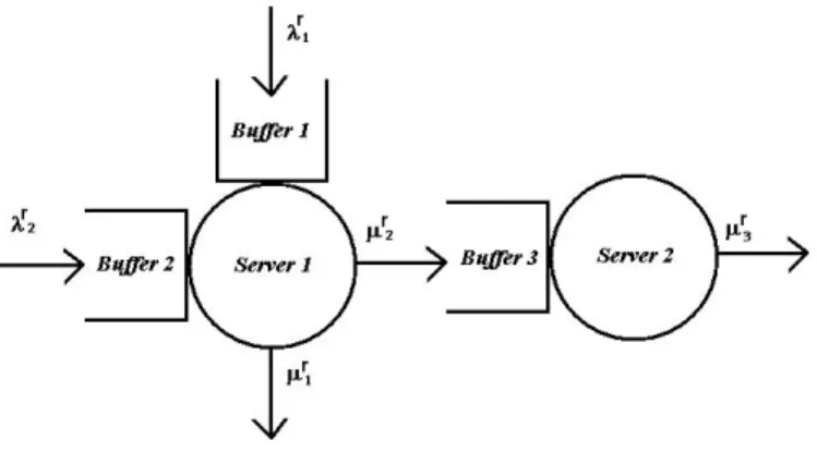
4.2 The Criss-Cross Network . . . 95
4.3 The Brownian Control Problem . . . 96
4.4 Equivalent Workload Formulation of the BCP . . . 98
4.5 Connections between EWF and BCP . . . 100
4.6 A Further Reduction in Parameter Regime IIb . . . 101
4.7 Equivalence between Singular Control and Optimal Stopping Problems . 103 4.8 Proof of Theorem 4.7.1 . . . 105
4.9 Numerical Study . . . 115
LIST OF FIGURES
2.1 State space and directions of control . . . 15
2.2 The discrete state space Sh`+ . . . 22
2.3 Numerically computed optimal control . . . 67
4.1 The criss-cross network . . . 96
4.2 Comparison of approximately optimal controls . . . 117
4.3 Divergence of numerical algorithm for singular control MDP . . . 119
4.4 Convergence of algorithm for optimal stopping MDP . . . 120
4.5 Algorithm for singular control MDP based on optimal stopping . . . 122
4.6 Approximate value function for singular control MDP . . . 122
Chapter 1
Introduction
Stochastic Control Theory is an active area of research in applied probability with ap-plications in diverse disciplines such as aerospace engineering, management science, eco-nomics, mathematical finance, and queuing networks. The area is quite well developed and now there are several excellent texts that are available ([19], [18], [30], [32], [52]). The basic problem can be described as follows. There is a stochastic dynamical system whose evolution can be influenced by exercising a control with a view towards achieving a desired goal. For example, if the dynamical system is described via a stochastic dif-ferential equation then a control may be in terms of modifying the drift or the diffusion coefficient. The control may be modulated continuously over time. It could be a bounded function of the current and past states of the controlled process or it may be unbounded, of the singular or impulsive type. Frequently, the desired goal in a stochastic control problem is to optimize a cost (or reward) function which may depend on both the state process and the control. From a computational point of view the main objective is to compute the minimal cost function, the so-calledvalue function, and the control policies that either achieve or well approximate this optimal cost.
so-called, Hamilton-Jacobi-Bellman (HJB) partial differential equations (PDEs). Rarely can such nonlinear PDEs be solved explicitly and thus in practice one needs to resort to numerical approximations. For diffusion control problems where the value function has suitable smoothness properties and is the unique classical solution of the corresponding HJB equation, there are well established finite difference methods that can be used for computing such approximations. However, many interesting modern applications involve diffusion control problems where due to degeneracies in the dynamics, non-smoothness of the boundary, singular nature of the control process, form of the boundary condition and other complexities, the associated value function is not necessarily smooth and the existence/uniqueness theory of the corresponding HJB equations is not well understood. Despite the fact that over the past twenty-five years there has been a rapid development in the theory ofviscosity solutionsof HJB equations for such diffusion control problems (cf. [10], [18], [49]), the PDE approach to the approximation of the value function becomes much more difficult.
problem as various approximation parameters approach suitable limits. This convergence analysis is completely probabilistic and is based on the theory of weak convergence of probability measures (e.g. [4]).
Although every Markov chain approximation corresponds to some particular finite difference approximation of the corresponding HJB equation, there are two main ad-vantages of the above probabilistic approach to the approximation problem. First, the Markov chain approach is flexible, and it enables use of physical insights derived from dynamics of the controlled diffusion in choosing the approximating chain, or equivalently, the precise form of the finite difference approximation. It is well known that if the finite difference approximation is not chosen appropriately, it may lead to serious instabilities in the numerical procedure. Markov chain approximations allow one to naturally select the appropriate finite difference scheme for a given application. Frequently, numerically unstable schemes can be avoided by incorporating such insights. Second, Markov chain approximation schemes do not require smoothness of the cost or value functions; nor do they rely on associated HJB equations. This is a great advantage in many problems where complex features of the dynamics make the PDE theory for the associated HJB equation hard to tackle, as is true for problems in the current work.
Singular control is perhaps one of the most difficult classes of problems in stochastic control theory. We refer the reader to [5], especially the sections at the end of each chapter, for a thorough survey of the literature. The HJB equations for such problems, which are variational inequalities with gradient constraints, are notoriously difficult to work with. Finite difference approximations for some singular control problems have been studied in [26] and [50]. In particular, the problem we study in Chapter 2 is precisely the one undertaken in [50]. However, our approach to the approximation problem is quite different in that all our techniques are probabilistic. We follow the Markov chain approach of Kushner and Dupuis and in contrast to [50] we prove convergence of the approximation scheme. Markov chain approximations along with convergence proofs for a singular control problem have been studied by Kushner and Martins in [33]. Although the work in Chapter 2 borrows significantly from the ideas in [33], specific features of the dynamics and the model under consideration make the convergence analysis quite delicate. In particular, the model features that make our analysis considerably harder than that in [33] include: unboundedness of the cost function, domain and control space, mixed boundary conditions (Dirichlet-Neumann), degeneracies in the dynamics and presence of both singular and absolutely continuous control. The main convergence result of the chapter is Theorem 2.4.12. This result, and the corresponding proofs, illustrate how the Markov chain approach can be adapted to handle complex dynamical features. While the analysis is for a specific two-dimensional problem, we believe that many of the techniques introduced in this chapter can be applied more generally.
Thus, whenever possible one would like to take advantage of specific problem features to simplify the numerical scheme. One such simplification results from exploiting con-nections between singular control and so-called obstacle/optimal stopping problems (see [45]). Although numerical schemes for singular control problems are notoriously hard, there are relatively simple schemes available for optimal stopping problems.
compact-ness arguments are developed in [40, 25, 15]. The first of these papers considers linear dynamics while the last two consider models with nonlinear coefficients. In all three papers the state space is all of IRd, i.e. there are no state constraints. It is important
to note that, in our model, although the drift and diffusion coefficients are constant, the state constraint requirement introduces a (non-standard) nonlinearity in the dynamics. While our method does not provide any characterization of the optimal control, it is quite general and should be applicable for other families of singular control problems (with or without state constraints).
The existence result of Chapter 3 (Theorem 3.2.3) is critical to establishing con-nections between singular control and optimal stopping problems. In Chapter 4 we investigate such connections for a two-dimensional singular control problem that arises from a scheduling control problem for the so-called criss-cross network (see Figure 4.1). This network has been studied by several authors (see [24], [9], [34], [38], and [8]). In the current work, we focus on the parameter regime IIb of [38], (Condition 4.6.1 of the current work), a regime which to date has not yielded an analytical solution. Using Theorem 3.2.3, we establish in Theorem 4.7.1 equivalence between the singular control problem and an optimal stopping problem. In Section 4.9 we exploit this connection to develop a computational scheme for the singular control problem which is much simpler than one based on a Markov chain approximation of the controlled process. The main idea is to numerically approximate the optimal stopping time and value function of the optimal stopping problem, and then use these quantities and Theorem 4.7.1 to obtain an approximation to the optimal control and value function for the singular control problem. Through several examples we illustrate how such an algorithm performs better numeri-cally than one based on a Markov chain approximation for the original singular control problem.
numbers is denoted as IR+. All vectors are column vectors and vector inequalities are
to be interpreted componentwise. For x ∈ IRn, |x| denotes the Euclidean norm. For a
point x∈IRn and a set A∈IRn, dist(x, A) will denote the distance of x fromA. Given
a Polish space E, a function f : [0,∞) → E is RCLL if it is right-continuous on [0,∞) and has left limits on (0,∞). We define the class of all such functions by D([0,∞) :E). The subset of D([0,∞) : E) consisting of all continuous functions will be denoted by
C([0,∞) :E). A process is RCLL if its sample paths lie in D([0,∞) :E) a.s. For T ≥0 and φ ∈ D([0,∞) : E) let |φ|∗
T
.
= sup0≤t≤T |φ(t)|. The Borel σ-field for a Polish space E will be denoted byB(E). We will denote generic constants in (0,∞) byc, c1, c2,· · ·; their
values may change from one theorem (lemma, proposition) to the next. By convention, the infimum of an empty set is ∞.
Chapter 2
Convergent Numerical Scheme for a
Problem of Optimal Consumption
and Portfolio Selection with
Transaction Costs
2.1
Problem Description and Motivation
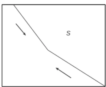
transfer money from the bank account to stock and vice-versa by paying a proportional transaction cost; namely, there are λ ∈ (0,∞) and µ ∈ (0,1) such that the investor pays λ times the amount moved from the bank account to stock as a transaction fee, and similarly, he pays µ times the amount moved from stock to the bank account as a transaction fee. All transaction fees are charged from the bank account. The basic constraint on the consumption control C and the portfolio selection control, denoted (M, N), is that the investor must be solvent at all times. More precisely, if X(t) and Y(t) represent the amount of investment in the bank account and the stock, respectively, at timet, then we require (X(t), Y(t))∈S for all t ≥0, where
S=. {(x, y)∈IR2 :x+ (1 +λ)y≥0 and x+ (1−µ)y≥0}.
The goal of the investor is to maximize the expected total discounted utility of consump-tion,IER0∞e−βtf(C(t))dt, whereβ ∈(0,∞) is the discount factor and the utility function
f : [0,∞)→[0,∞) is a continuous function satisfyingf(0) = 0. The conditionf(0) = 0 can be relaxed if f is nondecreasing and f(0)>−∞by replacing f by f−f(0).
In absence of transaction costs, Merton proved in the classical paper [41] that when the utility function isf(c) =cp/p, p <1, p6= 0 orf(c) = logc(note that the latter utility
attempts to exit the no-transaction region. The formal arguments of [36] were put on a rigorous footing by Davis and Norman in [12] for the casesf(c) =cp/porf(c) = logc. In
their work, under suitable conditions on model parameters, the free boundary problem associated with optimal consumption in the presence of proportional transaction costs is solved explicitly andC2 regularity of the value function is established. The authors show
that the (optimal) no-transaction region is a wedge, in particular, the optimal policy is to exercise the minimal amount of trading necessary to keep wealth inside the no-transaction region. Inside the region, consumption occurs at a finite rate. In [48] Shreve and Soner consider the same problem as in [12] but with conditions on the model parameters that are weaker and much more explicit. Once more, regularity properties of the value function and the associated free boundary are proved. A more general utility function which satisfies suitable smoothness, concavity and growth properties was considered in [50]. Using viscosity solution methods the authors sketch a proof for unique solvability of the associated HJB equation by the value function. A finite difference approximation scheme for approximating the value function is introduced; however, convergence of the proposed scheme for the portfolio selection problem is not proved. The authors do provide results from several numerical studies which identify near optimal control policies and the (numerical) free boundary.
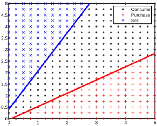
approximation approach their limits suitably. In Section 2.5 we use the approximating MDP to obtain computational schemes for obtaining near optimal control policies. The key result of Section 2.5 is Lemma 2.5.1, which allows us to characterize the value function and optimal control policies via solution of suitable dynamic programming equations (see Theorem 2.5.2). Finally in Section 2.6 results from a numerical study using the algorithm of Section 2.5 are described. In particular, Figure 2.3 shows the numerical no transaction region and the associated (numerical) free boundary obtained by an implementation of the algorithm.
inward into the state space (see Figure 2.1) and therefore do not allow for a similar Skorohod reduction. Nonetheless, one useful feature of the dynamics (see (2.1)) is that once the state of the system reaches the boundary of S, the only admissible control corresponds to moving the state process instantaneously to the origin and keeping it there at all times. This observation allows us to convert an infinite horizon cost to an exit time criterion (see equations (2.2)-(2.4)). This reformulation makes some aspects of the convergence analysis simpler, however, degeneracies in the state dynamics make treatment of convergence properties of exit times quite subtle. To see the basic difficulty consider the following simple example. Let ξn be a sequence of positive reals such that
ξn →0 asn→ ∞. Letxn be the solution of the ODE ˙x=xwith initial conditionξnand
x the solution of the same ODE with 0 initial condition. Clearly xn → x uniformly on
compacts, however ifτn = inf. {t|xn(t) = 0}and τ = inf. {t|x(t) = 0}, then clearly τn6→τ.
In other words, convergence of processes in general need not imply the convergence of the corresponding exit times. The issue is especially problematic when, as is the case for the controlled dynamics considered in this chapter, the diffusion coefficients in the state dynamics are not uniformly non-degenerate. This is another key difference between the current model and the problem studied in [33].
exercising the singular control. In the current problem there is no direct contribution to the (cost) reward function from the singular control term and as a result, the proof of this uniform estimate becomes more involved. Roughly speaking, the main idea of the proof is that a controller cannot make too much use of a singular control without pushing the process to the boundary of the domain.
The chapter is organized as follows. In Section 2.2 we give a precise formulation of the control problem of interest. We also present here two propositions (Propositions 2.2.2 and 2.2.4) which allow approximation of the original control problem by one with a bounded state space and bounded consumption actions. Section 2.3 introduces the discrete MDP that approximates the original singular control problem. It also introduces the continuous time interpolations and the time transformation that are key to the convergence analysis. In Section 2.4 we present the main convergence result that establishes the convergence of the value function of the MDP to that of the original singular control problem. Section 2.5 is devoted to computational methods for the MDP. A key result here is Lemma 2.5.1 which allows, via Theorems 2.5.2 and 2.5.3, iterative methods for computation of the value function and optimal control policies for the MDP. In problems with only absolutely continuous controls, estimates of the form in Lemma 2.5.1 are straightforward consequences of a contraction property that follows from the strictly positive discount factor in the cost (cf. Chapter 6 of [32]). However for singular control problems, due to the instantaneous nature of the control, such contraction estimates are typically unavailable. Here, once again, we use the special feature of the dynamics, which says that too much use of the singular control will rapidly bring the process to the boundary, in obtaining such an estimate. Finally, in Section 2.6 we present results from a numerical study of the algorithm.
a sequence of random variables {ξn}n≥0, we will use the notation δξn for the increment
ξn+1−ξn.
2.2
Optimal Consumption and Portfolio Selection
with Transaction Costs
We begin with a precise mathematical formulation of the optimal consumption-investment problem described in the previous section. Let (Ω,F, IP) be a probability space on which is given a filtration{Ft}t≥0 satisfying the usual hypothesis. LetW be a real-valued{Ft}
-Brownian motion. We will denote the probability system (Ω,F, IP,{Ft}, W) by Φ. The
Wiener process represents the source of uncertainty of the risky asset. The state process, which represents the wealth of the investor, is a controlled Markov process Z ≡ (X, Y) given on the above probability system via the equations:
dX(t) = (rX(t)−C(t))dt−(1 +λ)dM(t) + (1−µ)dN(t),
dY(t) = bY(t)dt+σY(t)dW(t) +dM(t)−dN(t), (2.1)
with initial condition X(0−) = x, Y(0−) = y, where z = (x, y). ∈ S . Here C is an {Ft}-progressively measurable process such that for all t ∈ [0,∞), C(t) ≥ 0 a.s.
and IER0te−rsC(s)ds < ∞. Also, M and N are {F
t}-adapted, non-decreasing, RCLL
S
Figure 2.1: State space and singular control directions.
the boundary of S. From the dynamical description of Z it follows that if z ∈ ∂S then the only control that keeps the investor solvent takesZ to the origin instantly and keeps it there at all times (see Figure 2.1).
Recall the utility function f of Section 2.1. Since f(0) = 0, one can reformulate the state constraint control problem on an infinite time horizon described in Section 2.1 to an exit time control problem, as follows. For z ∈ S and U ∈ A(z), let τ ≡ τ(z, U) be defined as
τ = inf. {t∈[0,∞) :Z(t)∈/ So}, (2.2)
where Z is the controlled process corresponding to initial condition z and control U. Define the cost,J(z, U), for using the control U by
J(z, U)=. IE
Z
[0,τ)
e−βtf(C(t))dt. (2.3) The value function of the control problem is then given by
V(z) = sup
Φ
sup
U∈A(z)
J(z, U), (2.4)
where the outside supremum is over all probability systems Φ. The following will be a standing assumption in this chapter.
We refer the reader to [28, 48, 50] for some sufficient conditions for the above assumption to hold.
State and Control Space Truncation. In order to develop numerical methods for computing V(z), we will need to first approximate the control problem by an analo-gous control problem with a bounded state space and control set. We now present the convergence result which says that the value function of the “truncated control prob-lem” converges to V as the truncation parameters approach their limits. We begin by considering the control space truncation.
For p ∈ (0,∞), let Ap(Φ, z) ≡ Ap(z) be the subset of A(z) consisting of U =
(C, M, N) which satisfy 0 ≤ C(t) ≤ p, for all t ≥ 0, a.s. Define Vp(z) by replacing A(z) withAp(z) in (2.4). The following is the first convergence result.
Proposition 2.2.2 Vp converges to V, uniformly on compact subsets of S, as p→ ∞.
Proof. We first establish pointwise convergence, i.e. Vp(z) → V(z) as p → ∞. Since
Vp(z)≤V(z), it suffices to show that, for all z ∈S,
lim inf
p→∞ Vp(z)≥V(z).
Fix² >0 and choose an “²-optimal control”, i.e. U² ∈ A(z) such thatV(z)−² < J(z, U²).
Suppose τ² is the associated exit time from So. Define a control ˜Up ≡ ( ˜Cp,M˜p,N˜p) by
˜
Cp(t) =. C²(t)∧p, ˜Mp(t) =. M²(t), ˜Np(t) =. N²(t), t ≥ 0. It follows from the fact that
˜
Cp ≤C²and standard comparison results for solutions of stochastic differential equations
(cf. Proposition 5.2.18 of [29]) that the wealth process under control ˜Up is never less than
the wealth process under control U². In particular, denoting by τp the exit time from So
by the controlled process corresponding to the control ˜Up, we have τp ≥ τ². Combining
continuous, we have from Fatou’s lemma
lim inf
p→∞ J(z,
˜
Up)≥lim inf p→∞ IE
Z
[0,τ²)
e−βtf( ˜C
p(t))dt ≥ IE
Z
[0,τ²)
e−βtf(C
²(t))dt ≥V(z)−².
Since² >0 is arbitrary, the pointwise convergence of Vp toV follows. Next we show that
for each p, Vp is lower semicontinuous (l.s.c.) Fix z ∈ S and let S 3 zn → z as n → ∞.
To prove that Vp is l.s.c. it suffices to show that
lim inf
n→∞ Vp(zn)≥Vp(z). (2.5)
Fix ² > 0 and let U² = (C², M², N²) ∈ Ap(z) be an ²-optimal control, i.e. Vp(z)−² <
J(z, U²). Let Z² be the controlled process according toU² and define τ² via (2.2) withZ
replaced by Z². Define Un ≡ (Cn, Mn, Nn) as Cn =. C², Mn(t) =. M²(t)1t<τ²+Mn∗1t≥τ²,
Nn(t) =. N²(t)1t<τ² + Nn∗1t≥τ², where Mn∗, Nn∗ ≥ 0 are chosen so that the controlled
process Zn corresponding to Un and initial condition zn satisfies Zn(τ²) ∈/ So. (Note,
clearly Un ∈ Ap(zn).) This insures that τn = inf. {t : Zn(t) ∈/ So} is at most τ². Note
that on the set{τ² =∞}, we have Un(t) =U²(t) for all t ≥0. We claim that on the set {τ² <∞} we have lim infn→∞τn ≥ τ² a.s., which implies τn → τ² a.s. as n → ∞ on the
set {τ² < ∞}. To see the claim, suppose that lim infτn < τ²−δ for some δ > 0. Then
there existsN0 ≥1 such that τn < τ²−δ/2 for all n ≥N0. Also, from the choice of the
controlUn we see that, for allδ >0 andL∈(0,∞), sup0≤t≤(τ²−δ/2)∧L|Zn(t)−Z(t)| →0,
in probability, as n → ∞. Combining this with the fact that Zn(τn) ∈/ So we have that
Z(t)∈/ So for some t≤ τ
²−δ/2. However, this contradicts the definition of τ². Thus we
have shownτn→τ² a.s. on the set {τ² <∞}.
{τ² =∞}, we have
Vp(z)−Vp(zn) ≤ J(z, U²)−J(zn, Un) +²
= IE
h
1{τ²<∞}
Z
[τn,τ²)
e−βt(f(C
²(t))−f(Cn(t)))dt
i
+²
≤ f∗(p)IE
h
1{τ²<∞}
Z
[τn,τ²)
e−βtdti+²,
wheref∗(p)= sup. 0≤c≤pf(c)<∞. Since τn →τ² a.s. on the set{τ²<∞}, the first term
on the right in the last line above approaches 0 as n → ∞. The inequality (2.5) now follows from the above display on taking n → ∞ and then² →0. Finally note that for eachz, V(z)−Vp(z)↓0. The result now follows from Dini’s Theorem (cf. Theorem M8
[4]).
Next, we consider the truncation of the state space. The reduction will be achieved by replacing the original dynamical system given by (2.1) with one which evolves exactly as before in the interior of some compact domain but is instantaneously reflected back when the controlled process is about to exit the domain. The reflection mechanism is made precise via the notion of a Skorohod map. We begin with the following definition. Fix`∈(0,∞).
Definition 2.2.3 Let φ ∈ D =. D([0,∞) : IR2) be such that φ(0) ∈ (−∞, `]×(−∞, `].
We will denote the space of all such φ by D0. We say a pair (ψ, η)∈ D × D solves the
Skorohod problem (SP) forφ in(−∞, `]×(−∞, `], with normal reflection, if the following hold: (i)ψ(0) =φ(0). (ii) ψ(t) = φ(t)−η(t), t∈(0,∞). (iii) ψ(t)∈(−∞, `]×(−∞, `] for all t ≥0. (iv) η(·) is componentwise nondecreasing. (v) ηi(t) =
R
(0,t]1{ψi(t)=`}dηi(t),
i= 1,2, where η(t) = (η1(t), η2(t))0, ψ(t) = (ψ1(t), ψ2(t))0.
It is well known (cf. [16], [22]) that for everyφ ∈ D0, there is a unique solution (ψ, η) to
the above SP. We will writeψ = Γ(φ) and refer to the map Γ : D0 → D0 as the Skorohod
There exists κ∈(0,∞), independent of `, such that, for allφ1, φ2 ∈ D0,
|Γ(φ1)−Γ(φ2)|∗T ≤κ|φ1−φ2|∗T, T ∈(0,∞). (2.6)
We will now introduce the modified constrained dynamics of the controlled Markov process. Set S`=. S∩(−∞, `]×(−∞, `]. LetZ` ≡(X`, Y`) solve the following system of
equations:
dX`(t) = (rX`(t)−C(t))dt−(1 +λ)dM(t) + (1−µ)dN(t)−dR1(t),
dY`(t) = bY`(t)dt+σY`(t)dW(t) +dM(t)−dN(t)−dR2(t), (2.7)
where Z`(0−) = z, U ≡ (C, M, N) ∈ Ap(z), z = (x, y) ∈ S` and R = (R1, R2)0 is a
componentwise nondecreasing, RCLL,Ft-adapted process satisfying
Z ∞
0
1{X`(t)<`}dR1(t) = 0,
Z ∞
0
1{Y`(t)<`}dR2(t) = 0. (2.8)
The unique solvability of (2.7) and (2.8) follows from the Lipschitz continuity property (2.6) of the Skorohod map and the usual Picard iteration method. Defineτ` and J`(z, U)
as in (2.2) and (2.3) withZ replaced byZ` in (2.2) and τ replaced byτ` in (2.3). Define
V`,p as
V`,p(z) = sup
Φ
sup
U∈Ap(Φ,z)
J`(z, U). (2.9)
The following is the second convergence result of this section.
Proposition 2.2.4 For all p∈(0,∞), V`,p converges to Vp, uniformly on compact
sub-sets of S, as `→ ∞.
such that
sup
Φ (M,Nsup)
sup
z∈S0
IE sup
0≤t≤T∧τ(X
+(t) +Y+(t))≤Λ,
where the supremum is taken over all {F(t)}-adapted, nondecreasing, RCLL processes M and N such thatM(0)≥0, N(0) ≥0; and over all systems Φ. Thus in particular we have that
sup
` supΦ U∈Asupp(Φ,z)
sup
z∈S0
IE sup
0≤t≤T∧τ`
(X`+(t) +Y`+(t))≤Λ, (2.10) whereZ` ≡(X`, Y`) are as defined in (2.7), and τ` is as introduced below (2.8).
Fix δ > 0. Let z ∈ S0 and ² > 0 be arbitrary. Let Φ and U ∈ Ap(z,Φ) be such
that V`,p(z) ≤ J`(z, U) + ². Choose T ∈ (0,∞) such that f∗(p)e−βT/T < ². Then
V`,p(z)≤IE
RT∧τ`
0 e−βtf(C(t))dt+ 2².
Choose `0 ≡`0(δ) such that `0 >(Λf∗(p))/(δβ). Define
A`0 .
={ω: sup
0≤t≤T∧τ`
(X+
` (t) +Y`+(t))> `0}.
Then
IE
Z T∧τ`
0
e−βtf(C(t))dt=IE[ 1A`0
Z T∧τ`
0
e−βtf(C(t))dt] +IE[ 1Ac `0
Z T∧τ`
0
e−βtf(C(t))dt]. (2.11) It follows from Markov’s inequality and (2.10) thatIP[A`0]≤Λ/`0. Thus the first integral on the right side of (2.11) is bounded by (f∗(p)/β)IP[A`0] ≤ δ. Next, for ` ≥ `0, on the setAc
`0, Z`(· ∧T ∧τ`) =Z(· ∧T ∧τ`). In particular, T ∧τ ≥T ∧τ`. Thus
IE[ 1Ac `0
Z T∧τ`
0
e−βtf(C(t))dt]≤IE[
Z T∧τ
0
e−βtf(C(t))dt] ≤ V p(z).
Combining the above bounds, we haveV`,p(z)≤Vp(z) +δ+ 2². Since² >0 is arbitrary,
we have that, for all ` ≥ `0 and z ∈ S0, V`,p(z) ≤ Vp(z) +δ. It is easily seen that the
δ >0, there exists an`0 such that|V`,p(z)−Vp(z)| ≤δ if ` > `0, for all z ∈S0. SinceS0
is an arbitrary compact subset ofS, the result follows.
Corollary 2.2.5 For all z ∈S, limp→∞lim`→∞V`,p(z) = V(z).
2.3
An Approximating Markov Decision Problem
In this section we will present the Markov decision problem whose value function ap-proximatesV`,p. Since throughout this section`, p will be fixed, we will drop them from
the notations: V`,p, τ`, J`,Ap(z) and Z` ≡ (X`, Y`). We will introduce a discrete time,
discrete state controlled Markov chain to approximate the continuous time process given by (2.7).
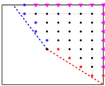
Fixh >0 and define the two-dimensionalh-grid,Lh =. {(jh, kh) :−∞< j, k <+∞}.
The symbol h denotes the approximation parameter and as h approaches 0, a suitable interpolation of the controlled Markov chain, to be introduced below, “approaches” a controlled diffusion process of the form in (2.7). We will assume for simplicity that ` is an integer multiple of h.
A natural definition of the state space for the approximating chain is Sh
` =. S`∩Lh.
However, due to reflection terms in the dynamics of the controlled process, it is convenient to consider a slightly “enlarged” state space, namely, Sh`+ =. S`+h ∩Lh. The “solvency
boundary” of the spaceSh+
` is defined as
∂h =. {(x, y)∈Sh+
` :x+ (1 +λ)y≤h(1 +λ) or x+ (1−µ)y ≤h}.
The points (x, y) ∈Sh+
` for which x= `+h or y= `+h form the reflecting boundary,
∂h
R.
Let{Zh
n, n= 0,1,2, . . .} be a discrete time controlled Markov chain with state space
Sh+
Figure 2.2: The discrete state space Sh`+.
evolution law well approximates the local behavior of the controlled diffusion (2.7). For each n, the increments of the chain δZh
n will approximate exactly one of the following
dynamical descriptions:
• “Controlled diffusion step”: (rXt−Ct, bYt)0dt+ (0, σ)0dWt.
• “Purchase control step”: (−(1 +λ),1)0dM
t.
• “Sales control step”: (1−µ,−1)0dN
t.
• “Reflection step”: dRt.
Each of these steps is described precisely in what follows. We also introduce a family of “interpolation intervals” {∆h, h > 0} used in defining the approximating cost function
and in the convergence arguments. For each pair (z, c) ∈ Sh+
` ×[0, p] we first define a
family ˜∆h(z, c). For the controlled diffusion steps, if the state of the chain is z and the
exercised consumption control is c, ∆h will be taken to be ˜∆h(z, c); whereas for singular
control steps and reflection steps ∆h will be taken to be 0. This reflects the fact that
for the controlled diffusion (2.7), reflection and singular control terms can change the state instantaneously. Suitable conditions on ˜∆h(z, c) in order to obtain convergence
of the continuous time interpolated processes to corresponding controlled diffusions are introduced below.
consistent” in the sense of [32], with a (controlled) diffusion given as:
dX(t) = (r˜ X(t)˜ −C(t))dt, dY˜(t) = bY˜(t)dt+σY˜(t)dW(t).
Formally, given h > 0, we choose for each c ∈ [0, p] and z ∈ Sh+
` \ ∂h a probability
measure qh(0)(z, c, d˜z) on Lh along with an interpolation interval ˜∆h(z, c) which satisfy
the following local consistency conditions for some ρ >0 :
m0(z, c) =.
Z
Lh
(˜z−z)qh(0)(z, c, d˜z) =
rx−c
by
∆˜h(z, c) +O(hρ∆˜h(z, c)), (2.12)
σ0(z, c) =.
Z
Lh
(˜z−z−m0(z, c))(˜z−z−m0(z, c))0q(0)h (z, c, dz)˜
=
0 0
0 |σy|2
∆˜h(z, c) +O(hρ∆˜h(z, c)). (2.13)
In the above displays ˜z = (˜x,y) and throughout, by the symbol˜ O(k) we will mean an expression which is bounded above by α|k|where α is a constant depending only on the coefficients of the model and the truncation parameters`, p. In addition we assume that there existsζ ∈(0,∞) such that qh(0)(z, c, Bζh(z)) = 1 for all c∈[0, p] and h > 0, where
Bζh(z) is a ball of radius ζh centered at z. The interpolation intervals are required to
satisfy:
˜ ∆h
∗
. = sup
z,c
˜
∆h(z, c)→0 as h→0, inf z,c
˜
∆h(z, c)>0 for each h >0, (2.14)
where the sup and inf in the above displays are taken over all (z, c) ∈ Sh+
` ×[0, p]. For
hr|x|+hp+hb|y|+σ2y2. Define for all (x, y)∈Sh+
` \∂h:
q(0)h ((x, y), c,(x+h, y))=. hrx+
Q(x, y) , q
(0)
h ((x, y), c,(x−h, y))
.
= hrx−+hc Q(x, y) ,
qh(0)((x, y), c,(x, y+h))=. hby
++1 2σ2y2
Q(x, y) , q
(0)
h ((x, y), c,(x, y−h))
. = hby
−+ 1 2σ2y2
Q(x, y) ,
qh(0)((x, y), c,(x, y)) =. h(p−c) Q(x, y), ˜
∆h(z, c) =. h
2
Q(x, y). (2.15)
It is easy to check that qh(0),∆˜h defined above satisfy (2.12), (2.13) and (2.14).
Singular Control Steps. The singular control terms in the controlled diffusion are the nondecreasing RCLL processes M and N. The process M pushes the state process in the direction v1 = (−(1 +λ),1)0, whereas N pushes the state process in the direction
v2 = ((1 −µ),−1)0. For the approximating chain we will assume that at most one
among the sales control and purchase control are exercised at any given time instant and the magnitude of the corresponding displacement is O(h). In order to capture the “singular” behavior of the limit diffusion — namely the feature that the state process can instantaneously be displaced by large amounts — we will take the interpolation interval for all singular control steps in the approximating chain to be 0.
In order to obtain weak convergence of the interpolated chain to the controlled dif-fusion, we need to ensure that the control directions match asymptotically those for the physical problem. More precisely, givenh >0 we define for eachz ∈Sh+
` two probability
measures q(hi)(z, d˜z), i= 1,2, on Lh as follows. For states (x, y)∈Sh+
` \∂h:
qh(1)((x, y),(x−h, y)) =λ/(λ+ 1) , qh(1)((x, y),(x−h, y+h)) = 1/(λ+ 1);(2.16) q(2)h ((x, y),(x, y−h)) =µ , qh(2)((x, y),(x+h, y−h)) = 1−µ. (2.17)
conditions:
mi(z) =.
Z
Lh
(˜z−z)q(hi)(z, d˜z) =hvi, (2.18)
σi(z) =.
Z
Lh
(˜z−z−mi(z))(˜z−z−mi(z))0qh(i)(z, d˜z) =O(h2). (2.19) Reflection Steps. We will define a transition kernel that with probability 1 moves a state in ∂h
R to some state in S
h
`. Once more, since reflection in the diffusion control
problem occurs instantaneously, we take the interpolation interval at reflection steps to be 0. Since the directions of reflection in the diffusion control problem are normal, a natural choice of the transition kernel for reflection step is as follows forz ∈∂h
R:
qh(3)((`+h, y),(`, y)) = 1, qh(3)((x, `+h),(x, `)) = 1, q(3)h ((`+h, `+h),(`, `)) = 1. (2.20)
For z /∈ ∂R, q(3)h (z,·) can be defined arbitrarily. It will be seen from the definition of admissible controls given below that for such states the definition of q(3)h is immaterial.
The Controlled Markov Chain. As described above, the control at each step is first specified by the choice of an action: controlled diffusion, singular control, or reflection. Therefore, we define a sequence of control actions{Ih
n, n= 0,1,2, . . .}with Inh = 0,1,2,3
if the nth step in the chain is a controlled diffusion step, purchase control step, sales control step, or a reflection step, respectively. In the case of a controlled diffusion step, the magnitude of the consumption control must also be specified. Consequently, the space of controls is given byU =. {0,1,2,3} ×[0, p].
ph(z, u, d˜z) on Lh by:
ph(z, u, d˜z) =qh(0)(z, c, d˜z) 1{i=0}+qh(i)(z, d˜z) 1{i∈{1,2,3}}. (2.21)
The definition of the transition function forz ∈∂h is not important since in the analysis
of the control problem the chain will be stopped the first time it hits ∂h. For sake of
specificity we setph(z, u, z) = 1 for allz ∈∂h and u∈ U.
We are now ready to specify the controlled Markov chains. Given a sequence Uh = {Uh
n, n = 0,1,2, . . .}(where Unh = (Inh, Cnh)) of U-valued random variables we construct a
controlled Markov chain {Zh
n, n = 0,1,2, . . .} with initial condition zh = (xh, yh) ∈ Sh`+
and state space Sh+
` , as follows:
Z0h =zh, IP[Znh+1 ∈E|Fnh] = ph(Znh, Unh, E), n ≥0, E ∈ B(Sh`+), (2.22)
where Fh
n = σ{Z0h, . . . , Znh, U0h, . . . , Unh}. The following definition of admissible controls
ensures thatZh
n ∈Sh`+ for all n and so the definition in (2.22) is meaningful.
Definition 2.3.1 The control sequence Uh ={Uh
n, n = 0,1,2, . . .} is said to be
admissi-ble for the initial conditionzh and{Znh}({Znh, Unh}) is called the corresponding controlled
Markov chain (resp. controlled pair) if:
1. Uh
n isσ{Z0h,· · · , Znh, U0h,· · · , Unh−1}-adapted.
2. IP[Ih
n = 3|Znh ∈Sh`] = 0 and IP[Inh = 3|Znh ∈∂Rh\∂h] = 1 for all n.
3. Condition (2.22) holds.
We also define for eachz ∈Sh`+ and u= (i, c)∈ U the interpolation intervals
∆h(z, u) = ˜∆h(z, c) 1
{i=0}. (2.23)
For an admissible pair {Zh
n, Unh}, we denote the associated sequence of interpolation
intervals ∆h(Zh
n, Unh) by {∆hn, n = 0,1,2, . . .}. Define, th0
.
= 0 and th n
.
= Pni=0−1∆h i for
n≥1.
Markov Decision Problem (MDP) for the Chain. Given an admissible pair
{Zh
n, Unh} let ηh = inf. {n : Znh ∈ ∂h}. The cost function for the controlled Markov
chain is defined as:
Jh(zh, Uh) = IE ηXh−1
n=0
e−βthnf(Ch
n)
³1−e−β∆h
n
β
´
. (2.24)
Note that we have used the factor (1−e−β∆h
n)/β rather than the more intuitive (and
asymptotically equivalent) ∆h
n. This somewhat simplifies the convergence proofs without
affecting the limiting results. The value function of the MDP is defined as:
Vh(z
h) = sup Uh∈Ah(z
h)
Jh(z
h, Uh). (2.25)
Continuous Time Interpolation. One of the main goals of the study is to show that the value function of the MDP defined in (2.25) converges, ash→0, to the value function of the limit diffusion control problem. This convergence result allows the computation of near optimal policies for the diffusion control problem introduced below (2.6) by numer-ically solving the above MDP. We next introduce the continuous time interpolation and time rescaling techniques that will be used in the proof of our main convergence result.
The continuous time interpolations of various processes will be constructed to be piecewise constant on the time intervals [th
we define nh(t) = max. {n : th
n ≤ t}, t ≥ 0. Note that nh(t) is an {Fnh}-stopping time.
Setting Fh(t) =. Fh
nh(t) we obtain a continuous time filtration {Fh(t), t ≥ 0}. Define
Uh(t) =. Uh
nh(t), t ≥ 0. Also, define the continuous time processes associated with the
controlled diffusion steps as follows. First letBh
0 = 0 and S0h = 0 and define for n≥1,
Bh n =.
n∧Xηh−1
k=0
IE[δZh
k|Fkh] 1{Ih
k=0}, S
h n =.
n∧Xηh−1
k=0
³
δZh
k −IE[δZkh|Fkh]
´
1{Ih
k=0}. (2.26)
Define the continuous time processBhby setting Bh(0)= 0 and. Bh(t)=. Bh
nh(t) fort >0.
The process Sh is defined in a similar manner. We define the interpolations associated
with the purchase control and sales control as follows. Let Mh
0 = 0, N0h = 0, Ei,h0 = 0,
i= 1,2 and define for n ≥1:
Mh n
. =
n∧Xηh−1
k=0
h1{Ih
k=1}, N
h n
. =
n∧Xηh−1
k=0
h1{Ih
k=2}, E
h i,n
. =
n∧Xηh−1
k=0
(δZh
k −hvi) 1{Ih k=i}.
The continuous time processes Mh and Nh are defined as Mh(0) = 0, N. h(0) = 0 and.
Mh(t) =. Mh
nh(t), Nh(t)
. = Nh
nh(t) for t ≥ 0. The processes E1h and E2h are defined
analo-gously. The continuous time process associated with reflection is defined as follows. If nh(t) = 0 define Rh(t) = 0; otherwise let
Rh(t)=. − nh(t)−1
X
k=0
δZh k1{Ih
k=3}. (2.27)
We define the continuous time interpolationZh of the controlled Markov chainZh n
intro-duced in Definition 2.3.1 byZh(t)=. Zh
nh(t), t≥0. The following representation forZh(t)
is easily verified:
Also, it follows from condition (2.12) that on the set {Ih
n = 0, ηh > n},
IE[δZnh|Fnh] =
rX
h n −Cnh
bYh n
∆h(Znh,0, Cnh) +O(hρ∆h(Znh,0, Cnh)) a.s.
This fact, together with the piecewise constant nature of the processes, yields
Bh(t) =
Z t∧τh
0
rX
h(s)−Ch(s)
bYh(s)
ds+δh
1(t), (2.29)
where τh =. th
ηh and δ
h
1 is an {Fh(t)}-adapted process which, in view of (2.14), satisfies
for all t≥0 and m≥1
sup
0≤s≤tIE|δ h
1(s)|m →0 as h→0.
A similar calculation gives the following representation of the cost function (2.24):
Jh(z
h, Uh) =IE
Z
[0,τh]
e−βtf(Ch(t))dt. (2.30) Time Rescaling. A common approach for proving the convergence of Vh to V as
h → 0 is to begin by showing that the collection {(Zh(·), τh), h ≥ 0} is tight and then
characterize the subsequential weak limits suitably. However, for problems with singular controls, showing the tightness of the above family becomes problematic since, in general, the processes {(Mh(·), Nh(·)), h ≥ 0} may fail to be tight. A powerful method for
handling this tightness issue was introduced by Kushner and Martins [37]. The basic idea is to suitably stretch out the time scale so that the various processes involved in the convergence analysis, in the new time scale, are tight; carry out the weak convergence analysis with the rescaled processes; and finally revert back to the original time scale to argue the convergence of Vh toV.
increments, {∆ˆh
n, n = 0,1,2, . . .}, are defined as ˆ∆nh = ∆. hn1{Ih
n=0} +h1{Inh∈{1,2}}. Define
ˆ th
0 = 0 and ˆ. thn=.
Pn−1
i=0 ∆ˆhi for n≥1.
Definition 2.3.2 The rescaled time processTˆh(t)is the unique continuous nondecreasing
process satisfying: (1) Tˆh(0) = 0; (2) the derivative of Tˆh(t) is 1 for t ∈ (ˆth
n,ˆthn+1) if
Ih
n = 0; (3) the derivative of Tˆh(t) for t∈(ˆthn,tˆhn+1) is 0 if Inh = 1,2,3.
It is easy to check that ˆTh(ˆth
n) = thn and that ˆTh(ˆthn+1)−Tˆh(ˆthn) = ∆hn. Let ˆnh(t)
. = max{n : ˆth
n≤t}, t≥0. Using the observation that every reflection step must be followed
by either a singular control step or a diffusion control step, it follows that ˆnh(t) is a
bounded{Fh
n}-stopping time, with bound
ˆ
nh(t)≤2³t
h +
t
infz,c∆ˆh(z,0, c)
´
<∞. (2.31)
Define the continuous time filtration{Fˆh(t), t≥0} by setting ˆFh(t)=. F
ˆ
nh(t).
The rescaled processes (denoted with a ˆ ) are defined in a manner similar to the processes defined below (2.26) with appropriate adjustments to the time variable. For example, we define ˆBh(0) = 0 and ˆBh(t)=. Bh
ˆ
nh(t) if ˆnh(t)> 0. We define the processes
ˆ
Uh(t), ˆSh(t), ˆMh(t), ˆNh(t), ˆEh
1(t), ˆE2h, ˆRh(t), ˆZh(t) analogously (that is, by replacing
nh(t) with ˆnh(t) in the definitions below (2.26)). Then we have the following rescaled
version of (2.28)
ˆ
Zh(t) = z
h+ ˆBh(t) + ˆSh(t) +v1Mˆh(t) +v2Nˆh(t) + ˆE1h(t) + ˆE2h−Rˆh(t). (2.32)
Remark 2.3.3 From the definition of Tˆh(t) if follows that nˆh(t) = nh( ˆTh(t)). This
equality yields a straightforward relationship between the original interpolated processes
and the rescaled processes. For example, Bˆh(t) = Bh( ˆTh(t)). Similar equations hold
between Uh(t), Sh(t), Mh(t), Nh(t), Eh
1(t), E2h, Rh(t), Zh(t) and their corresponding
Using the fact that ˆTh(ˆth
n+1)−Tˆh(ˆthn) = ∆hn which is 0 for singular control and reflection
steps, a calculation similar to that which produced (2.29) yields
ˆ Bh(t) =
Z t∧ˆτh
1 0 r ˆ
Xh(s)−Cˆh(s)
bYˆh(s)
dTˆh(s) + ˆδh1(t), (2.33)
where ˆτh
1
.
= inf{t : ˆZh(t) ∈ ∂h} and ˆδh
1 is an {Fˆh(t)}-adapted process satisfying for all
m≥1,
IE sup
0≤s≤t |δˆh
1(s)|m →0 as h→0. (2.34)
We now state several lemmas related to the time rescaling. The following “change of variables” formula (cf. Theorem IV.3.45 [43]) will be used several times in our analysis.
Lemma 2.3.4 Let Gˆ : [0,∞) → [0,∞) be a continuous and nondecreasing function. Suppose that G(t)ˆ → ∞ as t → ∞. Define the inverse G : [0,∞) → [0,∞) as G(t) = inf{s: ˆG(s)> t}. Then for all bounded and measurable functions g : [0,∞)→[0,∞),
Z
[0,G(t)]
g(s)dG(s) =ˆ
Z
[0,t]
g(G(s))ds. (2.35)
The following lemma is at the heart of the time transformation idea. It ensures that the weak limits of ˆTh(t) increase to ∞ as t → ∞ and thus makes the reverting back to the
original time scale, in the limit, possible (see Theorem 2.4.6).
Lemma 2.3.5 Let {Uh
n, n = 0,1,2, . . .}h>0 be a family of admissible control sequences.
Then for allt ≥0
sup
h
IE|Mh(t) +Nh(t)|<∞. (2.36)
Proof. Without loss of generality, assume h∈(0,1). Define
Yh i (t)
. =
nh(t)∧η h−1
X
δZh k1{Ih
k=i} , n
h i(t)
. =
nh(t)∧η h−1
X
1{Ih
WritingYh
i ≡(Yi,h1, Yi,h2)0, it follows from (2.16) and (2.17) that,
IEYh
1,2(t) =h
1 1 +λIE[n
h
1(t)], IEY2h,1(t) =h(1−µ)IE[nh2(t)].
A straightforward calculation shows|Bh(t)| ≤c
1(1 +t) and IE|Sh(t)| ≤c2(1 +t), where
the constantsc1,c2 are independent ofh andt. From (2.16), (2.17) we see that hnh1(t) =
Mh(t) =Yh
1,1(t) and hnh2(t) =Nh(t) = Y2h,2(t). Thus from (2.28) there is ˜c1 ∈(0,∞) such
that
hnh1(t)≤c˜1(1 +t) +|S1h(t)|+Y2h,1(t), hnh2(t)≤˜c1(1 +t) +|S2h(t)|+Y1h,2(t). (2.37)
Combining the above inequalities we have, for somec3 ∈(0,∞),hIE[nh1(t)]≤c3(1 +t) +
h(1−µ)IE[nh
2(t)] andhIE[nh2(t)]≤c3(1 +t) +hIE[nh1(t)]/(1 +λ).It follows thathIE[nh1(t)]
and hIE[nh
2(t)] are “close” to each other. More precisely, there exist constants α ≥ 1,
c4 >0,L0 >0 such that for L≥L0
h(IE[nh
1(t)]∨IE[nh2(t)])> L⇒h(IE[n1h(t)]∧IE[nh2(t)])> αL−c4.
In particular, we have suphhIE[nh
1(t)] = ∞if and only if suphhIE[nh2(t)] =∞. Now
sup-pose suphhIE[nh
1(t)] = ∞and suphhIE[nh2(t)] =∞. By Cramer’s theorem (see Theorem
2.1.24 [13]), for allδ > 0 there exists a constant c(δ)∈(0,∞) such that for allk0 ∈IN0
and h >0
max
n
IP[|Y2h,1−h(1−µ)n2h(t)|> δhnh2(t), nh2(t) =k0],
IP[|Yh
1,2−h(1/(1 +λ))nh1(t)|> δhnh1(t), nh1(t) = k0]
o
²∈(0,1) and choose K large enough so that
c(δ) 1−e−c(δ)e
−c(δ)(K+1) < ²
8 and
c2(1 +t)
θK−˜c1(1 +t)
< ²
8. (2.38)
Since, by assumption suphhIE[nh
1(t)] = suphhIE[nh2(t)] = ∞, there exists h0 ≤ 1 such
that
IP[nh0
1 (t)>
K h0, n
h0
2 (t)>
K
h0]> ². (2.39)
Then for all t≥0,
IP[|Yh0
2,1(t)−h0(1−µ)nh
0
2 (t)|> δh0nh
0
2 (t), nh
0
2 (t)>
K h0]
=
∞
X
j=[K/h0]+1
IP[|Y2h,10(t)−h0(1−µ)n2h0(t)|> δh0nh20(t), nh20(t) =j]
≤
∞
X
j=[K/h0]+1
c(δ)e−c(δ)j = c(δ)
1−e−c(δ)e
−c(δ)([K
h0]+1) < ²
8,
where the last inequality follows from the choice of K in (2.38). Similarly, IP[|Yh0
1,2(t)− h
0
1+λnh
0
1 (t)|> δh0nh
0
1 (t), nh
0
1 (t)> Kh0]< ²8.Hence, in view of (2.39) we have
IP[|Yh0
2,1(t)−h0(1−µ)nh
0
2 (t)| ≤δh0nh
0
2 (t),
|Yh0
1,2(t)−
h0
1 +λn
h0
1 (t)| ≤δh0nh
0
1 (t),min{nh
0
1 (t), nh
0
2 (t)}>
K h0]>
² 2.
LetE denote the event in the equation above. From (2.37) and (2.38)
IP[h0nh0
1 (t)−Yh
0
2,1(t)≥θK] ≤ IP[|Sh
0
1 (t)| ≥θK−˜c1(1 +t)]
≤ IE|S h0
1 (t)|
θK−˜c1(1 +t)
≤ c2(1 +t)
θK−˜c1(1 +t)