Sparse Nonlinear Feature Selection Algorithm via Local Structure Learning

(1)

Emerging Science Journal

Vol. 3, No. 2, April, 2019

Sparse Nonlinear Feature Selection Algorithm via Local

Structure Learning

Jiaye Li

a*

_{, Guoqiu Wen}

a

_{, Jiangzhang Gan}

a

_{, Leyuan Zhang}

a

_{, Shanwen Zhang}

a

a _{Guangxi Normal University, Guilin 541004, China}

Abstract

In this paper, we propose a new unsupervised feature selection algorithm by considering the nonlinear and similarity relationships within the data. To achieve this, we apply the kernel method and local structure learning to consider the nonlinear relationship between features and the local similarity between features. Specifically, we use a kernel function to map each feature of the data into the kernel space. In the high-dimensional kernel space, different features correspond to different weights, and zero weights are unimportant features (e.g. redundant features). Furthermore, we consider the similarity between features through local structure learning, and propose an effective optimization method to solve it. The experimental results show that the proposed algorithm achieves better performance than the comparison algorithm.

Keywords: Feature Selection;

Kernel Function;

Local Structure Learning;

High-Dimensional.

Article History:

Received: 28 February 2019 Accepted: 07 April 2019

1- Introduction

With the advent of the digital age, a large amount of data has been generated. These data is difficult to deal with in terms of human capabilities and efficiency [1]. At this point, data mining and machine learning are born. In many learning tasks in machine learning (e.g., classification, clustering et al.), it is often difficult to process high-dimensional [2] data. Moreover, in many cases, the processing time and amount of calculation of the model are greatly improved when processing high-dimensional data. Therefore, it is necessary to use the feature selection algorithm [3-5] to preprocess (i.e., dimensionality reduction) high-dimensional data.

Feature selection is the selection of a subset of features that represent the overall characteristics of the data [6, 7]. In the existing feature selection algorithms, they often apply different weights to different features through a sparse regularization factor, thereby selecting relatively important features [26-29]. For example, Zhu proposes Local and Global Structure Preservation for Robust Unsupervised Spectral Feature Selection, which maintains the local structure of features by feature self-expression and maintains a global representation of features by low rank representation of sparse regularization factors. This method also uses local structure learning to maintain the local structure of the sample points. However, there are still some limitations to the existing feature selection algorithms that need to be addressed.

First, there are some feature selection algorithms that take into account the similarity between sample points, although it can take into account the local structural information of the data to some extent. But it has not been applied to the features, which is a small flaw. After considering the similarity of features, we can find that among some similar features, only a part of the features can be selected. Because it is clear that in similar features, the probability of having redundant features is large. Secondly, according to the kernel function in SVM, we can know that in low-dimensional space, only the linear relationship between features can be mined. When the features are mapped into a high-dimensional space, the

*_CONTACT_:_{[email protected]}

DOI:http://dx.doi.org/10.28991/esj-2019-01175

(2)

nonlinear relationship between the features is linearly separable in the high-dimensional space. In this way, the relationship within the feature can be more fully explored, thus making the mining more thorough.

This paper proposes a new unsupervised feature selection algorithm to deal with the above two problems. Specifically, for the nonlinearity of the feature, we use a Gaussian kernel function to map each feature to a kernel matrix and then apply a weight to each feature. The important feature pairs have a large weight value, and the relatively unimportant feature (i.e., redundant feature) corresponds to a weight value of zero. For the similarity of features, we use local structure learning to consider the similarity between features. At the same time, the local structure of the feature can be maintained. For our proposed algorithm, we adopt the method of alternating iterative optimization, so that the algorithm is gradually decremented in each iteration, and finally reaches convergence. The main contributions we have listed for our approach are as follows.

 The similarity and non-linear relationship between features are considered simultaneously on a framework. The

relationship between features is more fully explored through kernel sparse learning and local structure learning, thus effectively removing redundant features.

 The global structure of the data is maintained by low rank constraints, and complements the local structure learning.

At the same time, low rank constraints can also remove noise samples and outliers, which improves the robustness of the algorithm to some extent.

 We propose an algorithm of alternating iterative optimization to solve our objective function. The method

gradually reduces the value of the objective function in each iteration and finally converges. At the same time, we also use theory to prove the convergence of our proposed algorithm. The experimental results also show that compared with other comparison algorithms, our proposed algorithm achieves better results on real data sets.

2- Related Work

Feature selection is an important way of data pre-processing. It mainly looks for a subset of features that represent the original data. Due to the popularity of sparse learning, most of the existing feature selection algorithms use sparse learning. However, from the perspective of machine learning, the existing feature selection algorithms are mainly divided into unsupervised feature selection algorithm, semi-supervised feature selection algorithm and supervised feature selection algorithm.

In the unsupervised feature selection algorithm of the past two years, Almusallam et al. proposed an efficient unsupervised feature selection for streaming features [8]. The algorithm uses the K-means algorithm to aggregate features that are not known into a feature stream. It uses three independent similarity measures to determine whether to add existing features to the subset features by calculating the similarity measure. Wan et al. proposed global and intrinsic geometric structure embedding for unsupervised feature selection [11]. This method takes into account the information difference between the original feature space and the low-dimensional subspace. The projection matrix is constrained

by the 𝑙₂ or 𝑙_2,1− norm to select more sparse and more discriminative properties.

At the same time, some new feature selection algorithms have been proposed in the last two years. For example, Xue et al. proposed online weighted multi-task feature selection [9]. This paper proposes a weighted multitasking model that not only selects important features, but also sparse solutions. At the same time, the convergence speed of the algorithm is also guaranteed. Liu et al. proposed global and local structure preservation for feature selection [10]. The article mainly states that it is extremely important to maintain the global similar structure and local geometry of the data for supervised feature selection algorithms. For the unsupervised feature selection algorithm, it is more important to maintain the local geometry of the data. Li et al. proposed a stable feature selection algorithm [12]. The algorithm is a stable feature

selection algorithm based on energy learning. It uses 𝑙₁ or 𝑙₂ regularization term to investigate its stability. Tsagris et al.

proposed feature selection for high-dimensional temporal data [13]. The algorithm extends the constraint based feature selection algorithm for high-dimensional temporal data, and finally achieves good results.

(3)

3- Our Method

In this section, we first introduce the symbols used in this article and then explain our proposed Unsupervised Feature Selection Algorithm via Local Structure Learning and Kernel Function(Abbreviated as: LSK FS) , in Sections 3.1 and 3.2, respectively, and then optimize the proposed optimization method in Section 3.3. Finally, we analysis the convergence of the objective function in Section 3.4.

3-1- Notations

For the data matrix _ n d

X R , the i-th row and the j-th column are denoted as i

X andXj respectively, and the elements

of the i-th row and the j-th column are denoted as xi j, . The trace of the matrix X is denoted bytr(X),

T

X denotes the

transpose of the matrix X, and 1

X represents the inverse of the matrix X. We also denote the norm and norm of X

respectively as 2 2

2 2

n i d

j F i x  j x

X and

1 1

d j j X 



_ x .

3-2- LSK FS Algorithm

Suppose a given sample data set_Χ_ n d

R , where n and d represent the number of samples and the number of attributes,

respectively.

This paper first breaks the data set_Χ_ n d

R into d column vectors, each vector 1

, 1,..., n i

xR i d. Then it treats each

element in eachxi as an independent feature valuexijR, j = 1,...,n. And projects them into the kernel space to get the

kernel matrix ( )i_ n n

K R , namely:

1 1 1 2 1

2 1 2 2 2

( )

1 2

( , ) ( , ) ( , )

i i i i i in

i

in i in i in in

k x x k x x k x x

k x x k x x k x x

 

 

_ _

 

 

K

… …

… … … …

…

(1)

Thus the original _ n d

X R becomes d kernel matrices.

The unsupervised feature selection algorithm mainly mines more representative features in the data. In the absence

of the class label Y, using the data matrix X as a response matrix, the internal structure of the original features of the

data can be better preserved [18, 19]. In order to fully exploit the nonlinear relationship of data features. Get the following expression:

( ) 1

d i i i

α 





Χ K W

(2)

Where _ n d

W R represents the kernel coefficient matrix, _{α R}_ d1_{is used to perform feature selection, which is equivalent}

to the weight vector of the feature, αi is an element of the vector α,

 i_ n n

Κ R is the kernel matrix.

Predecessors have proved that the local structure between data can be used to reduce the dimension [20], so this paper makes local structure learning by establishing a similarity matrix between data features in low-dimensional space. The following formula is obtained through local structure learning:

2 ,

, 2

min d T T

i j i j

i jx x s



Z W W (3)

Where n1

i

xR represents i-th feature. _ n d

W R is the conversion matrix of high-dimensional data in low-dimensional

space, si j, is an element of matrix S, indicating the similarity between featurexiand featurexj. If the featurexi is the

k-th nearest neighbor of k-the featurexj, then the valuesi j, is obtained by the Gaussian kernel function; otherwise =0. In order

to make X get a better fitting effect, and consider the structural relationship between data features in low-dimensional

space, we get the following formula:

2

2 ( )

1 , 2 ,

, , 1

min d

d

i T T

i i j i j i j

i F

α λ x x s













S W α X K W W W (4)

Since the similarity matrix S is particularly affected by the influence of parametersσ. In order to reduce the number

of adjustment parameters, a more efficient similarity matrix is learned. In this paper, structural learning and low-dimensional space learning are alternated to achieve their optimal results. Specifically get the following formula:

2

2 2

( )

1 , 2 , 2 2

, , 1

, ,

min

. ., , = 1,s 0, 0,if Ν( ), 0

d

i T T

i i j i j i j i

i F

T

i i i i j

α λ x x s λ s

s t i s s j i otherwise



   

   



S W α X K W W W

1

(5)

Where λ1,λ2 is the tuning parameter, si is the i-th column of the similar matrix S, and

2 2

i

s is used to avoid

(4)

order to maintain rotation invariance, we set T = 1 i

s 1 . Therefore, the above formula can make the similarity corresponding

to the feature having a relatively close distance large, and the feature having a relatively long distance has a small corresponding value.

In order to eliminate the interference of the outliers, the noise samples are removed at the same time [21]. This paper

adds a low rank constraint [22] to the matrix W, namely:



W AB (6)

Where _ n r

A R , _ r d

B R ,rmin( , )n d , we added an orthogonal limit to A, in order to fully consider the correlation

between the output variables. We add a l1norm of α for sparse learning and feature selection [23]. Finally we get our

final objective function as follows:

2

2 ( )

1 , 2 ,

, , , 1 2

2 2 3 1

,

min

. ., , = 1, s 0,

0, if Ν( ), 0,

d

i T T

i i j i j i j

i F

i T

i i i

T i j

α λ x x s

λ s λ

s t i s

s j i otherwise



  

 

 

  



1

S A B α X K AB AB AB

α

A A I

(7)

Where T _{ } r r

A A I R , λ1, λ2 and λ3 are the tuning parameter. The kernel matrix K is calculated by the Gaussian kernel

function, and its main function is to map the data to the kernel space, thereby mining the nonlinear relationship between

the data features. The l1norm of the last item α is used to sparse the features for feature selection. If the value of the

element corresponding to the vector α is zero, it means that the feature is not selected.

3-3- Optimization

Since the objective function is not co-convex, the closed solution cannot be directly obtained. Therefore, this paper proposes an alternate iterative optimization method to solve the problem, which is divided into the following four steps:

Update A by fixing S, α and B:

When S, α and B are fixed, the optimization (7) problem becomes:

2

2 ( )

1 , 2 ,

1

min

. .,

d

i T T

i i j i j i j

i F

T

α λ x x s

s t 

  





A X K AB AB AB

A A I

(8)

We make ( )

1

= d

i i i

α 



Ρ K , then the (8) formula can be transformed into:

2 2

1 , 2 ,

min

. .,

d _T _T

i j i j

F i j

T

λ x x s

s t

  





A X PAB AB AB

A A I

(9)

We simplify the (9), we have:

1

min ( )

( ), . .,

T T T T T T T T

T T T T

tr

λ tr s t

  

 

A X X X PAB B A P X B A P PAB

B A XLX AB A A I

(10)

Where tr( ) represents the trace of matrix, = - _ d d

L Q S R is a Laplace matrix, Q is a diagonal matrix, and the elements

of each column are , 1 ,

d

i i j i j

q 



_s . Deriving for A, we have:

1

2_λ T T_2 T T_2 T T

XLX ABB P XB P PABB (11)

Due to the orthogonality of A, we can optimize it by the method in [24].

Update B by fixing S, α and A

By fixing S, α and A, the objective function (7) can be simplified as follows:

2

2 ( )

1 , 2 ,

1

min d

d

i T T

i i j i j i j

i F

α λ x x s













B X K AB AB AB (12)

It is easy to get (12) is equivalent to the following formula:

1

min ( )

( )

T T T T T T T T

T T T

tr λ tr

  



B X X X PAB B A P X B A P PAB

B A XLX AB

(13)

When we ask for B and let its derivative be zero, we can get:

1 1

( T T _λ T T ) T T

 

(5)

Update S by fixing A, α and B

After fixing A, α and B, the objective function (7) becomes:

2 2

1 , 2 , 2 2

,

min

. ., , = 1, s 0,

0, if Ν( ), 0

d _T _T

i j i j i

i j T

i i i

i j

λ x x s λ s

s t i s

s j i otherwise

 

 

 



S AB AB

1 (15)

We first calculate the Euclidean distance between every two data features to construct the neighbours of all the

features. If the j-th feature does not belong to the nearest neighbour of the i-th feature, then the value of si j, is zero;

otherwise, the value of si j, is solved by equation (18).

At the same time, optimizing S is equivalent to optimizing each s ii( 1,..., )d individually, so we further translate the

optimization problem into the following equation:

, ,

2 ₂

1 , 2 ,

, 2

1 1,min0, 0 ( )

T i i i i j

d T T

i j i j i j

i j

s s s 



λ x ABx AB s λ s (16)

Here, _Z__Rd d _{, in which} 2

, 1 ₂

T T

i jλ xi xj

Z AB AB , such (16) further becomes:

, ,

2 1

1 1, 0, 0

2 2

min 2 T

i i i i j

i i

s s s

λ s

λ

    Z (17)

Under KKT conditions, we can get the following:

1

, ,

2

( )

2

i j i j

λ

s Z τ

λ 

   (18)

Since each data feature has a neighbour, we sort eachZ ii( 1,... )d in descending order, that isZˆi{Zˆi,1,...,Zˆi,d}, we know:

, 1 0

i k

s   ,si k, 0. We have:

1 , 1 2

ˆ ₀

2 i k λ

Z τ

λ 

   (19)

Under the conditions T = 1

i

s 1 , we can get:

1 1 , , 1 1 2 2 1 ˆ ˆ

( ) 1

2 2

k k

i k i k

j j

λ λ

Z τ τ Z

λ k kλ

      



(20)

Update α by fixing A, B and S

After fixing A, B and S, the objective function (7) becomes:

2 ( ) 3 1 1 min d i i i F α λ  





α X K AB α (21)

In order to optimize the next step, here is the simplification of the above formula, namely:

( ) ( )

(1) ( )

2

(1) ( )

1 3 1

2

(1) ( )

1 3 1

2

1 ,. ,. ₂ 3 1

1

min ( ... )

i i n d

d d d _F d d _F n

i i d i

i q q                     



       α Q K ΑΒ R

α

Χ K ΑΒ K ΑΒ α

Χ Q Q α

Χ α (22) We set (1) (1) ( ) ( ) ,1 , ( ) ,1 , d d

i i d

i d d

i i d

q q q q             

M R and have:

2 ( ) 3 1 2 1 2 ( ) 3 1 2 1 ( ) 1 1 ( ) ( ) 3 1 1 min

min ( )

min 2

( ( ) ) i i n T i i i n

T i T

i

n n

T T i T

i i

n

T i i T

i                  



α α α

Χ α M α

Χ M α α

Χ Χ α M Χ

α M M α α

(23)

(6)

2 ( ) 1

3 1

( )

( ) ( ) d

i i

i F

f α

F f λ



 

 



α X K AB

α α α

(24)

Note that α₁ is convex but not smooth. So using approximate gradient to optimizeα, we can update iterationsα by

the following rules.

1 arg min ( , )

t  _α Gηt t

α α α

(25)

      2

3 1

, ,

2 t

ηt t t t t t

η

G α α f α   f α α α   α α λ α

(26)

In the above formula, ( ) ( ) ( )

1 1

( )=2 ( ( ) ) 2 ( )

n n

T i i T i T

t t i

i i

f

 

 α α



M M 



X M , ηt is a tuning parameter, αt is the value of αin the t-th

iteration.

By ignoring the independence in equation (26), we can get:

2 ₃

1 1

1 ( ) arg min

2 t

t η t _α t F

t λ π

η

    

α α α U α

(27)

Where t t 1 ( )t

t f η   

U α α , ( ) t

η t

π α is the Euclidean projection on the convex setηt, because α1 has a separable form, the

formula (27) can be written as follows:

2 3

1 ₂

1 arg min

2 i

i i i i

t t

α

t λ

α α U α

η

   

(28)

Where_αi_and

1

i t

α_ are the i-th elements of α and αt1 respectively, then according to formula (28), 1

i t

α_ can obtain the

following closed solution:

3 3

* ( ), if

0, otherwise.

i i i

t t t

i

t t

λ λ

u sign u u

η η

α     

 (29)

To speed up the approximate gradient algorithm in equation (26), we have added auxiliary variables:

+1 1

+1

1

( )

t

t t t t

t β

β 



  

V α α α

(30)

Where

2 1

1 1 4

2 t t

β β_   

.

Algorithm 1. Pseudo code for solving (7) Input: _ n d

X R , 1, 2, 3, r, η0, β1=1, γ; Output: A, B, S, α;

1.Initialize t=1;

2.Randomly initialize (0)

A , (0)

B , and α0; 3.Compute (i)

K by formula (1); 4.Repeat

5.Update A via formula (8); 6.Update B via formula (12); 7.Update S via formula (15);

8.Update α according to the following rules 9.while F( )αt Gηt1



πηt1( ),α αt t



;

10.Set ηt1γηt1; 11. end while 12. Set ηtγηt1;

13. Compute αt1arg min_ Gηt( ,α Vt); 14. Compute

2 t t+1

1 1 4

2 β

β    ;

15. Compute formula(30) ; 16. t=t+1;

(7)

3-4- Convergence Analysis

According to (18), for alli j, 1,...,n, ( 1)

,

t i j

s  has a closed solution. We can get the following formula:

2

( ) ( ) ( ) ( ) ( ) ( ) ( ) ( 1)

1 , 2 ,

1 2 ( 1)

2 , 2

2

( ) ( ) ( ) ( ) ( ) ( ) ( ) ( )

1 , 2 ,

1 2 ( )

2 , 2

d

i t t T t t T t t t

i i j i j i j

i F d t i i j d d

i t t T t t T t t t

i i j i j i j

i F

d t

i i j

α λ x x s

λ s

α λ x x s

λ s             



X K A B A B A B

(31)

When α and ( 1)t

S are fixed, to update _A( 1)t _and_B( 1)t _{, we can get:}

2

( ) ( 1) ( 1) ( 1) ( 1) ( 1) ( 1) ( 1)

1 , 2 ,

1 2 ( 1)

2 , 2

2

( ) ( ) ( ) ( ) ( ) ( ) ( ) ( 1)

1 , 2 ,

1 2 ( 1)

2 , 2

d

i t t T t t T t t t

i i j i j i j

i F d t i i j d d

i t t T t t T t t t

i i j i j i j

i F

d t

i i j

α λ x x s

λ s

α λ x x s

λ s                     



X K A B A B A B

X K A B A B A B

(32)

From the above two types, we have:

2

( ) ( 1) ( 1) ( 1) ( 1) ( 1) ( 1) ( 1)

1 , 2 ,

1 2 ( 1)

2 , 2

2

( ) ( ) ( ) ( ) ( ) ( ) ( ) ( )

1 , 2 ,

1 2 ( )

2 , 2

d

i t t T t t T t t t

i i j i j i j

i F d _t i i j d d

i t t T t t T t t t

i i j i j i j

i F

d t

i i j

α λ x x s

λ s

α λ x x s

λ s                   



X K A B A B A B

X K A B A B A B

(33)

Theorem 1 let αt be the sequence generated by Algorithm 1, then for t 1, (34) holds:

2 * 1 * 2 2 ( ) ( ) ( 1) F t γL F F t     α α α α (34)

According to reference [38], γ is a constant defined in advance, L is the Lipschitz constant of the f( )α gradient in

equation (24), and *

arg min ( )F

 α

α α .

Through the above inequality and Theorem 1, we can easily see that our algorithm is convergent.

4-

Experiments

We compared the classification accuracy of our algorithm and 8 comparison algorithms in 12 data sets (shown in Table 1).

4-1- Experimental Settings

We tested our proposed unsupervised feature selection algorithm on four binary data sets and eight multi-class data sets. They are Yale, Colon, Lung_discrete, Glass, SPECTF, Sonar, Clean, Arrhythmia, Movements, Ecoli, Urban_land and Forest, where the first three data sets are from feature selection data, and the last nine data sets are from the UCI data set. The details of the data set are shown in Table 1:

Table1. The information of the data sets Datasets Samples Dimensions Classes

Glass 214 9 6

Movements 360 90 15

SPECTF 267 44 2

Ecoli 336 343 8

Sonar 208 60 2

(8)

Clean 476 167 2

Forest 325 27 4

Arrhythmia 452 279 13

Colon 62 2000 2

Yale 165 1024 15

Lungdiscrete 73 325 7

At the same time, we found eight representative feature selection comparison algorithms to compare with our proposed algorithm. The main introduction of the algorithm is as follows:

EUFS [30]: This paper proposes a new unsupervised feature selection algorithm, which is different from other unsupervised feature selection algorithms to generate tags through clustering algorithms. This method directly embeds feature selection into the clustering algorithm through sparse learning theory. The most prominent contribution of this method is that other unsupervised feature selection algorithms can be applied to this framework.

FSASL [31]: The intrinsic structure of the data is rarely considered for existing feature selection algorithms. By placing structural learning and feature selection in a framework at the same time, the algorithm can effectively select representative features while maintaining the structure of the data (i.e., structural learning and feature selection complement each other).

NDFS [32]: The algorithm is a new unsupervised feature selection algorithm that mines discerning information. Specifically, it imposes a non-negative constraint on the class indication to learn clustering tags more accurately. At the

same time, l2,1norm is used to remove redundant features. It is an algorithm that performs clustering and feature

selection simultaneously.

NetFS [33]: This method is also an unsupervised feature selection algorithm, but the algorithm is mainly for Networked Data. Due to the large amount of noise in Networked Data, the algorithm combines latent representation learning for feature selection. Through sparse learning and latent representation learning, the algorithm can remove the noise interference well and finally achieve good robustness.

RLSR [34]: This paper proposes a semi-supervised feature selection algorithm by finding the global and sparse

solutions of the projection matrix. The main contribution of the algorithm is to propose a regular term 2

2,1

l norm, and

gives a detailed theoretical proof, which proves that the regular term can effectively select features and take into account global information.

RFS [35]: This paper presents a new robust feature selection algorithm through sparse learning. Specifically, it

applies l2,1norm to both the loss function and the regular item. Sparse restriction on the regular term can effectively

remove the redundant features. The l2,1norm of the loss function can effectively remove the noise samples, thus

achieving a robust effect.

RSR [36]: The algorithm is a new unsupervised feature selection algorithm that learns by regularized

self-characterization. Specifically, if a feature is particularly important, it can be represented linearly by most other features (i.e., a feature can be represented by a combination of other features). In addition, the algorithm shows good performance on both manual and real data sets.

K_OFSD [37]: The algorithm is an online feature selection algorithm, which mainly selects relevant features through neighbor learning. Through this method, the class imbalance problem can be effectively solved. At the same time, the dimensionality of the high-dimensional data is effectively reduced by the dependency between the conditional features and the decision-making class.

In our proposed model, we set 2 2

1 2

{ , } {10 ,...,10 }λ λ _  _{, the rank of the kernel coefficient matrix}

{1,..., min( , )}

r n d , and the

parameter of l2,pnorm p{0.1,...,1.9}. The parameters

5 5

{2 ,..., 2 }

c  and 5 5

{2 ,..., 2 }

g  are used to select the best SVM for

classification. Through 10-fold cross-validation, we divide the data set into a training set and a test set. In order to minimize the experimental error, we perform 10 times experiments, and finally find the average of the classification accuracy.

Since the experiment uses the classification accuracy rate to measure the performance of the algorithm, we define the classification accuracy as follows:

/

correct

accX X (31)

Where X represents the total number of samples and Xcorrect represents the correct number of samples for classification.

(9)

2 1

1

( )

N i i

std acc μ

N 





 (32)

Where N represents the number of experiments, acci represents the classification accuracy of the i-th experiment, μ

represents the average classification accuracy, and the smaller the std, the more stable the representative algorithm.

4-2- Experiment Result

In Figure 1, we can clearly see the classification accuracy of the 10 experiments. The algorithm we proposed is not the highest every time, but most of the cases are the highest. In Table 2, we can see the average classification accuracy of each algorithm on 12 data sets. The algorithm proposed by us is obviously superior to other comparison algorithms. Specifically, it is 4.78% higher than EUFS in average classification accuracy and 5.05% higher than FSASL, which indicates that our algorithm is better than the general feature selection algorithm. Compared with K_OFSD, NDFS, NetFS, RLSR, RFS, and RSR. LSK_FS increased 13.63%, 8.55%, 6.69%, 7.88%, 6.68%, and 3.59%, respectively. In particular, our algorithm is particularly effective on the dataset SPECTF.

The number of experiments The number of experiments

Arrhythmia Clean

The number of experiments The number of experiments

Colon Ecoli

The number of experiments The number of experiments

Forest Glass

1 2 3 4 5 6 7 8 9 10

0 10 20 30 40 50 60 70 80

the number of experiments

ac

c(

%)

EUFSFSASL

K-OFSD NDFS NetFS RLSR RFS RSR LSK-FS

1 2 3 4 5 6 7 8 9 10

0 10 20 30 40 50 60 70 80 90 100

the number of experiments

ac

c

(%)

EUFS FSASL K-OFSD NDFS NetFS RLSR RFS RSR LSK-FS

1 2 3 4 5 6 7 8 9 10

0 10 20 30 40 50 60 70 80 90

the number of experiments

ac

c

(%)

1 2 3 4 5 6 7 8 9 10

0 10 20 30 40 50 60 70 80 90

the number of experiments

ac

c(

%)

1 2 3 4 5 6 7 8 9 10

0 10 20 30 40 50 60 70 80 90

the number of experiments

ac

c(

%)

1 2 3 4 5 6 7 8 9 10

0 10 20 30 40 50 60 70

the number of experiments

ac

c

(%)

(10)

The number of experiments The number of experiments

Lungdiscrete Movements

The number of experiments The number of experiments

Sonar SPECTF

The number of experiments The number of experiments

Urban_land Yale

Figure 1. Average classification accuracy of all methods for all datasets

1 2 3 4 5 6 7 8 9 10

0 10 20 30 40 50 60 70 80 90

the number of experiments

ac

c

(%)

1 2 3 4 5 6 7 8 9 10

0 10 20 30 40 50 60 70 80 90

the number of experiments

ac

c(

%)

1 2 3 4 5 6 7 8 9 10

0 10 20 30 40 50 60 70 80 90

the number of experiments

ac

c(

%)

1 2 3 4 5 6 7 8 9 10

0 10 20 30 40 50 60 70 80 90 100

the number of experiments

ac

c

(%)

1 2 3 4 5 6 7 8 9 10

10 20 30 40 50 60 70

the number of experiments

ac

c(

%)

1 2 3 4 5 6 7 8 9 10

10 20 30 40 50 60 70 80

the number of experiments

ac

c

(%)

(11)

Table 2. Average classification accuracy (acc(%))

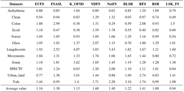
In Table 3, we can see the average standard deviation of each algorithm on 12 data sets. The standard deviation of the proposed LSK_FS algorithm is the smallest, indicating that our algorithm has the best stability.

Table 3. Standard deviation of classification accuracy (std(%))

Datasets EUFS FSASL K_OFSD NDFS NetFS RLSR RFS RSR LSK_FS

Arrhythmia 0.88 0.85 1.04 0.89 0.02 0.85 1.29 1.09 0.79

Clean 0.54 0.94 0.03 1.29 1.32 0.03 0.97 0.74 0.49

Colon 1.88 2.99 0.38 1.31 0.29 0.59 2.08 0.93 1.5

Ecoli 1.18 0.47 0.30 1.59 1.78 0.55 0.40 0.82 0.69

Forest 1.05 1.05 0.93 1.05 1.06 1.29 1.16 0.99 0.54

Glass 1.05 1.02 1.37 2.07 1.15 0.70 1.00 1.29 1.01

Lungdiscrete 1.92 2.52 4.07 3.03 3.43 1.82 1.67 1.21 1.60

Movements 1.04 1.31 1.33 1.76 1.06 1.65 1.44 0.80 0.72

Sonar 1.18 1.81 1.62 1.85 1.45 1.19 1.28 1.28 1.38

SPECTF 1.01 1.24 0.03 1.20 2.08 1.10 1.11 1.01 0.04

Urban_land 0.77 1.38 1.01 1.44 0.88 1.69 2.74 0.83 1.41

Yale 1.44 0.95 1.4 1.71 2.28 3.16 1.74 0.99 1.08

Average value 1.16 1.38 1.13 1.60 1.40 1.22 1.41 1.00 0.94

The LSK_FS algorithm can achieve such good results, mainly for the following two reasons: 1. Consider the similarity between data features. 2. Fully consider the nonlinear relationship between data features.

4-3- Parameter Sensitivity Analysis

We set the range of values for 1 and 2 to

2 1 2

{10 ,10 ,...,10 }  . By adjusting the values of parameters 1 and 2, we

show the results of our proposed algorithm in Figure 2.

As shown in Figure 2, the proposed algorithm is sensitive to adjusting parameters. Specifically, it is not very sensitive

on most data sets, but it also has subtle changes. This is because the algorithm proposed by us has better robustness. 1

is used to control the value of 2

,

, 2

d T T

i j i j

i jx x s

 AB AB , while , 22 ,

d T T

i j i j

i jx x s

 AB AB takes into account the nonlinear relationship

of the features.2 is used to control the value of

2 2

i

s , and 2

2

i

s takes into account the similarity of features. Therefore,

in our proposed algorithm, it is necessary to adjust the parameters.

Datasets EUFS FSASL K_OFSD NDFS NetFS RLSR RFS RSR LSK_FS

Arrhythmia 60.52 66.71 60.74 65.57 54.20 70.53 64..02 66.33 70.96

Clean 84.61 84.83 86.53 77.82 95.78 91.53 84.64 84.77 96.13

Colon 82.88 77.07 64.60 64.43 64.38 64.42 82.48 83.17 84.14

Ecoli 84.97 86.01 69.28 82.81 84.47 78.31 85.74 85.81 86.19

Forest 85.23 86.06 74.23 76.31 86.43 85.78 83.50 86.55 88.50

Glass 68.90 70.17 52.09 67.86 70.20 69.36 64.17 70.42 71.38

Lungdiscrete 86.11 86.07 75.45 82.77 73.41 84.43 85.88 85.55 86.41

Movements 81.36 81.61 71.19 86.61 81.42 73.58 72.08 88.61 88.92

Sonar 83.81 78.67 79.11 85.43 86.66 77.26 83.91 83.91 88.48

SPECTF 79.54 79.70 79.40 78.48 83.95 79.22 78.04 79.54 92.94

Urban_land 61.78 62.05 53.25 51.27 56.96 60.20 58.82 61.72 63.56

Yale 75.27 73.69 63.78 71.22 65.04 64.05 69.76 73.81 75.63

(12)

Arrtythmia Clean Colon

Ecoli Forest Glass

Lungdiscrete Movements Sonar

SPECTF Urban_land Yale

Figure 2. Accuracy of the proposed algorithm under different parameter values

4-3- Convergence Analysis

In Figure 3, we show the objective function values for each iteration of the proposed algorithm, on 12 data sets. We

set the stop criteria of the proposed algorithm to 4

( 1) ( ) ( ) 10

obj t obj t obj t   , where obj t( ) represents the value of the

objective function at the t-th iteration. From Figure 3 we can see that: 1. The proposed optimization algorithm is

(13)

Arrhythmia Clean Colon

Ecoli Forest Glass

Lungdiscrete Movements Sonar

SPECTF Urban_land Y ale

Figure 3. The convergence graph of algorithm 1 for all data sets

5- Conclusion

This article has proposed a new feature selection algorithm to remove redundant features. Specifically, the local structure learning is applied to the features to take into account the local structure and similarity of the features. Moreover, the kernel function is applied to map all the features in the high-dimensional space, so that the nonlinear relationship of the features is linearly separable in the high-dimensional space. In addition, low rank constraints are used to remove noise samples, maintain the global structure of the data and achieve robust results. Finally, the experimental results also show the superiority of our proposed algorithm. In future work, we plan to improve our algorithms through robust statistical learning.

6- Funding and Acknowledgements

This work is partially supported by the China Key Research Program (Grant No: 2016YFB1000905); the Key Program of the National Natural Science Foundation of China (Grant No: 61836016); the Natural Science Foundation of China (Grants No: 61876046, 61573270, 81701780 and 61672177); the Project of Guangxi Science and Technology

0 5 10 15 20

0 1 2

3x 10

4 Iteration times O b je c ti v e v a lu e

0 10 20

0 5000 10000 15000 Iteration times O b je c ti v e v a lu e

0 5 10 15 20

0 2 4 6 8x 10

0 10 20

1000 1010 1020 1030 1040 Iteration times O b je c ti v e v a lu e

0 10 20

0 5 10 15 20

0 1 2 3x 10

0 5 10 15 20

0 2 4 6

8x 10

0 10 20

(14)

(GuiKeAD17195062); the Guangxi Natural Science Foundation (Grant No: 2015GXNSFCB139011, 2017GXNSFBA198221); the Guangxi Collaborative Innovation Center of Multi-Source Information Integration and Intelligent Processing; the Guangxi High Institutions Program of Introducing 100 High-Level Overseas Talents; Innovation Project of Guangxi Graduate Education(Grant No: YCSW2019073) and the Research Fund of Guangxi Key Lab of Multisource Information Mining & Security (18-A-01-01).

7- Conflict of Interest

The authors declare no conflict of interest.

7- References

[1]X. Zhu, H. Suk and D. Shen, "Matrix-Similarity Based Loss Function and Feature Selection for Alzheimer's Disease Diagnosis," 2014 IEEE Conference on Computer Vision and Pattern Recognition, Columbus, OH, 2014, pp. 3089-3096. doi: 10.1109/CVPR.2014.395.

[2]Zhu, Xiaofeng, Zi Huang, Yang Yang, Heng Tao Shen, Changsheng Xu, and Jiebo Luo. “Self-Taught Dimensionality Reduction on the High-Dimensional Small-Sized Data.” Pattern Recognition 46, no. 1 (January 2013): 215–229. doi:10.1016/j.patcog.2012.07.018.

[3]Zhu, Xiaofeng, Shichao Zhang, Zhi Jin, Zili Zhang, and Zhuoming Xu. “Missing Value Estimation for Mixed-Attribute Data Sets.” IEEE Transactions on Knowledge and Data Engineering 23, no. 1 (January 2011): 110–121. doi:10.1109/tkde.2010.99. [4]Bolón-Canedo, Verónica, Noelia Sánchez-Maroño, and Amparo Alonso-Betanzos. “Feature Selection for High-Dimensional

Data.” Progress in Artificial Intelligence 5, no. 2 (February 15, 2016): 65–75. doi:10.1007/s13748-015-0080-y.

[5]Ling, Charles X., Qiang Yang, Jianning Wang, and Shichao Zhang. “Decision Trees with Minimal Costs.” Twenty-First International Conference on Machine Learning - ICML ’04 (2004). doi:10.1145/1015330.1015369.

[6]Zhang, Shichao, Zhi Jin, and Xiaofeng Zhu. “Missing Data Imputation by Utilizing Information Within Incomplete Instances.” Journal of Systems and Software 84, no. 3 (March 2011): 452–459. doi:10.1016/j.jss.2010.11.887.

[7]Nie F, Zhu W, Li X. (2016). Unsupervised feature selection with structured graph optimization[C]// Thirtieth AAAI Conference on Artificial Intelligence. AAAI Press, 2016:1302-1308.

[8]Almusallam, Naif, Zahir Tari, Jeffrey Chan, and Adil AlHarthi. “UFSSF - An Efficient Unsupervised Feature Selection for Streaming Features.” Lecture Notes in Computer Science (2018): 495–507. doi:10.1007/978-3-319-93037-4_39.

[9]Xue, Wei, and Wensheng Zhang. “Online Weighted Multi-Task Feature Selection.” Lecture Notes in Computer Science (2016): 195–203. doi:10.1007/978-3-319-46672-9_23.

[10]Xinwang Liu, Lei Wang, Jian Zhang, Jianping Yin, and Huan Liu ,“Global and Local Structure Preservation for Feature Selection.” IEEE Transactions on Neural Networks and Learning Systems 25, no. 6 (June 2014): 1083–1095. doi:10.1109/tnnls.2013.2287275.

[11]Wan, Yuan, Xiaoli Chen, and Jinghui Zhang. “Global and Intrinsic Geometric Structure Embedding for Unsupervised Feature Selection.” Expert Systems with Applications 93 (March 2018): 134–142. doi:10.1016/j.eswa.2017.10.008.

[12]Li, Yun, Jennie Si, Guojing Zhou, Shasha Huang, and Songcan Chen. “FREL: A Stable Feature Selection Algorithm.” IEEE Transactions on Neural Networks and Learning Systems 26, no. 7 (July 2015): 1388–1402. doi:10.1109/tnnls.2014.2341627. [13]Tsagris, Michail, Vincenzo Lagani, and Ioannis Tsamardinos. “Feature Selection for High-Dimensional Temporal Data.” BMC

Bioinformatics 19, no. 1 (January 23, 2018). doi:10.1186/s12859-018-2023-7.

[14]Zhao, Hong, Ping Wang, and Qinghua Hu. “Cost-Sensitive Feature Selection Based on Adaptive Neighborhood Granularity with Multi-Level Confidence.” Information Sciences 366 (October 2016): 134–149. doi:10.1016/j.ins.2016.05.025.

[15]Wang, Wei, Yan Yan, Stefan Winkler, and Nicu Sebe. “Category Specific Dictionary Learning for Attribute Specific Feature Selection.” IEEE Transactions on Image Processing 25, no. 3 (March 2016): 1465–1478. doi:10.1109/tip.2016.2523340. [16]Sheeja, T.K., and A. Sunny Kuriakose. “A Novel Feature Selection Method Using Fuzzy Rough Sets.” Computers in Industry

97;111–121 (May 2018): 111–116. doi:10.1016/j.compind.2018.01.014.

[17]Zhang, Tao, Biyun Ding, Xin Zhao, and Qianyu Yue. “A Fast Feature Selection Algorithm Based on Swarm Intelligence in Acoustic Defect Detection.” IEEE Access 6 (2018): 28848–28858. doi:10.1109/access.2018.2833164.

[18]Almusallam, Naif, Zahir Tari, Jeffrey Chan, and Adil AlHarthi. “UFSSF - An Efficient Unsupervised Feature Selection for Streaming Features.” Lecture Notes in Computer Science (2018): 495–507. doi:10.1007/978-3-319-93037-4_39.

(15)

195–203. doi:10.1007/978-3-319-46672-9_23.

[20]Liu X, Wang L, Zhang J, Yin Jianping and Liu Huan. “Global and Local Structure Preservation for Feature Selection.” IEEE Transactions on Neural Networks and Learning Systems 25, no. 6 (June 2014): 1083–1095. doi:10.1109/tnnls.2013.2287275. [21]Wan, Yuan, Xiaoli Chen, and Jinghui Zhang. “Global and Intrinsic Geometric Structure Embedding for Unsupervised Feature

Selection.” Expert Systems with Applications 93 (March 2018): 134–142. doi:10.1016/j.eswa.2017.10.008.

[22]Li, Yun, Jennie Si, Guojing Zhou, Shasha Huang, and Songcan Chen. “FREL: A Stable Feature Selection Algorithm.” IEEE Transactions on Neural Networks and Learning Systems 26, no. 7 (July 2015): 1388–1402. doi:10.1109/tnnls.2014.2341627. [23]Tsagris, Michail, Vincenzo Lagani, and Ioannis Tsamardinos. “Feature Selection for High-Dimensional Temporal Data.” BMC

Bioinformatics 19, no. 1 (January 23, 2018). doi:10.1186/s12859-018-2023-7.

[24]Zhao, Hong, Ping Wang, and Qinghua Hu. “Cost-Sensitive Feature Selection Based on Adaptive Neighborhood Granularity with Multi-Level Confidence.” Information Sciences 366 (October 2016): 134–149. doi:10.1016/j.ins.2016.05.025.

[25]Wang, Wei, Yan Yan, Stefan Winkler, and Nicu Sebe. “Category Specific Dictionary Learning for Attribute Specific Feature Selection.” IEEE Transactions on Image Processing 25, no. 3 (March 2016): 1465–1478. doi:10.1109/tip.2016.2523340. [26]Sheeja, T.K., and A. Sunny Kuriakose. “A Novel Feature Selection Method Using Fuzzy Rough Sets.” Computers in Industry

97 (May 2018): 111–116. doi:10.1016/j.compind.2018.01.014.

[27]Zhang, Tao, Biyun Ding, Xin Zhao, and Qianyu Yue. “A Fast Feature Selection Algorithm Based on Swarm Intelligence in Acoustic Defect Detection.” IEEE Access 6 (2018): 28848–28858. doi:10.1109/access.2018.2833164.

[28]Zhang, Chengqi, Yongsong Qin, Xiaofeng Zhu, Jilian Zhang, and Shichao Zhang. “Clustering-Based Missing Value Imputation for Data Preprocessing.” 2006: 1081-1086 IEEE International Conference on Industrial Informatics (August 2006). doi:10.1109/indin.2006.275767.

[29]Qin, Yongsong, Shichao Zhang, Xiaofeng Zhu, Jilian Zhang, and Chengqi Zhang. “Semi-Parametric Optimization for Missing Data Imputation.” Applied Intelligence 27, no. 1 (January 18, 2007): 79–88. doi:10.1007/s10489-006-0032-0.

[30]Wang, Suhang, Jiliang Tang, and Huan Liu. "Embedded unsupervised feature selection." In Twenty-ninth AAAI conference on artificial intelligence. 2015: 470-476.

[31]Du, Liang, and Yi-Dong Shen. “Unsupervised Feature Selection with Adaptive Structure Learning.” Proceedings of the 21th ACM SIGKDD International Conference on Knowledge Discovery and Data Mining - KDD ’15 (2015). doi:10.1145/2783258.2783345.

[32] Li, Zechao, Yi Yang, Jing Liu, Xiaofang Zhou, and Hanqing Lu. "Unsupervised feature selection using nonnegative spectral analysis." In Twenty-Sixth AAAI Conference on Artificial Intelligence. 2012: 1026-1032.

[33]Li, Jundong, Xia Hu, Liang Wu, and Huan Liu. "Robust unsupervised feature selection on networked data." In Proceedings of the 2016 SIAM International Conference on Data Mining, pp. 387-395. Society for Industrial and Applied Mathematics, 2016: 387-395.

[34]Chen, Xiaojun, Guowen Yuan, Wenting Wang, Feiping Nie, Xiaojun Chang, and Joshua Zhexue Huang. “Local Adaptive Projection Framework for Feature Selection of Labeled and Unlabeled Data.” IEEE Transactions on Neural Networks and Learning Systems 29, no. 12 (December 2018): 6362–6373. doi:10.1109/tnnls.2018.2830186.

[35]Nie, Feiping, Heng Huang, Xiao Cai, and Chris H. Ding. "Efficient and robust feature selection via joint ℓ2, 1-norms minimization." In Advances in neural information processing systems, pp. 1813-1821. 2010.

[36]Zhu, Pengfei, Wangmeng Zuo, Lei Zhang, Qinghua Hu, and Simon C.K. Shiu. “Unsupervised Feature Selection by Regularized Self-Representation.” Pattern Recognition 48, no. 2 (February 2015): 438–446. doi:10.1016/j.patcog.2014.08.006.

[37]Zhou, Peng, Xuegang Hu, Peipei Li, and Xindong Wu. “Online Feature Selection for High-Dimensional

Class-Imbalanced Data.” Knowledge-Based Systems 136 (November 2017): 187–199. doi:10.1016/j.knosys.2017.09.006.