and Corrected Adaptively
Truncated Likelihood Methods
by Harald Dornheim and Vytaras Brazauskas
AbstrAct
Two recent papers by Dornheim and Brazauskas (2011a, 2011b)
introduced a new likelihood-based approach for robust-efficient
fitting of mixed linear models and showed that it possesses
favor-able large- and small-sample properties which yield more
accu-rate premiums when extreme outcomes are present in the data. In
particular, they studied regression-type credibility models that can
be embedded within the framework of mixed linear models for
which heavy-tailed insurance data are approximately
log-location-scale distributed. The new methods were called corrected
adap-tively truncated likelihood
methods (or CATL, for short). In this
paper, we build upon that work and further explore how CATL
methods can be used for pricing risks. We extend the area of
appli-cation of standard credibility ratemaking to several well-studied
examples from property and casualty insurance, health care, and
real estate fields. The process of outlier identification, the ensuing
model inference, and related issues are thoroughly investigated on
the featured data sets. Throughout the case studies, performance
of CATL methods is compared to that of other robust regression
credibility procedures.
Keywords
1. Introduction
Credibility theory is one of the oldest but still most common premium ratemaking techniques in insur-ance industry, and it continues to attract the atten-tion of practicing actuaries and academic researchers. Since the publication of the first regression-linked credibility model (Hachemeister, 1975), numerous extensions, improvements, and practical applications of this model have been proposed in the actuarial lit-erature. Here is a short but representative list of recent papers on this topic:
• Frees, Young, and Luo (1999) gave a longitudi
-nal data a-nalysis interpretation of the standard (Bühlmann 1967; Bühlmann and Straub 1970) and other additive credibility ratemaking procedures. This interpretation also remains valid in the frame-work of mixed linear models. A few years later, the same authors presented several case studies
involv-ing such models (Frees, Young, and Luo 2001). • Fellingham, Tolley, and Herzog (2005) analyzed a
real data set provided by a major health insurance provider, which summarized claims experience for select health insurance coverages in Illinois and Wisconsin. Credibility methods, in conjunction with mixed linear models and Bayesian hierarchi-cal models, were used to make next-year predictions of claims costs.
• Guszcza (2008) provided an excellent introduction
to hierarchical models that can be viewed as an extension of traditional (linear) credibility models. Several hierarchical models were then used in a loss reserving exercise, to model loss development across multiple accident years.
• Klinker (2011) introduced generalized linear mixed
models (GLMM) as a way of incorporating cred
-ibility in a generalized linear model setting. The
application of a GLMM to a case study on ISO data
revealed connections between this approach and the Bühlmann-Straub credibility.
As is the case with many mathematical models, credibility-type models contain unknown structural
parameters (or, in the language of mixed linear
mod-els, fixed effects and variance components) that have
to be estimated from the data. For statistical inference
about fixed effects and variance components, tra-ditional likelihood-based methods such as (restricted) maximum likelihood estimators, (RE)ML, are com-monly pursued. However, it is also known that while these methods offer most flexibility and full efficiency at the assumed model, they are extremely sensitive to small deviations from the hypothesized normality of random components as well as to the occurrence of outliers. To obtain more reliable estimators for pre-mium calculation and prediction of future claims, vari-ous robust methods have been successfully adapted to credibility theory in the actuarial literature (see, for
example, Garrido and Pitselis 2000; Dornheim and Brazauskas 2007; Pitselis 2002, 2008).
At this point a short discussion about robust statistics—a well-established field in statistics—might aid the reader who is not familiar with this area. In a nutshell, robust statistics is concerned with model
mis-specification (or using the actuarial terminology,
model risk) and data quality (e.g., measurement errors, outliers, typos). The main focus is on parametric mod-els, their fitting to the observed data, and identification
of outliers. Fitting of the model, however, is accom -plished by employing procedures that are designed to have limited sensitivity to changes in the underlying assumptions as well as to “unexpected” data points. The procedures that possess such properties are called
robust. A very important tool for measuring perfor-mance of, and for providing guidance on how to con-struct robust estimators is the influence function (IF). The IF helps to quantify the estimator’s robustness
and efficiency, which usually are two competing cri-teria. Typically, robust and efficient estimators belong to one of three general classes of statistics: L-, M-, or
R-statistics. (Here, L stands for linear in the “linear combinations of order statistics”; M stands for
maxi-mum in the “maximum likelihood type statistics”;
R stands for ranks in the “statistics based on ranks”.) It is not uncommon, however, to have estimators that can be reformulated within more than one of these
M-statistics, for example, are arguably the most ame-nable to generalization and often lead to theoretically optimal procedures. R-statistics can be recast in the context of hypothesis testing and enjoy a close rela-tionship with the broad field of nonparametric sta-tistics. L-statistics are fairly simple computationally and have a straightforward interpretation in terms of quantiles.
Further, in the initial stages of its development,
research in the field of robust statistics was focused on quite simple parametric problems (e.g., estimation of the location parameter of a bell-shaped curve), but over the years it expanded into linear models, time series analysis and other more complex problems. Now, almost five decades later, the impact of robust statistics is felt in numerous applied and interdisciplin-ary areas, ranging from natural and social sciences to computer science, engineering, insurance, and finance. Robust procedures add the most value to the model-ing process when the underlymodel-ing model contains many unknown parameters and/or multiple assumptions, because the more complex the model, the higher the
chance to misspecify it. Finally, robust statistics is
parametric by its nature and thus differs from empiri-cal nonparametric methods which have no (or very weak) parametric assumptions. The main advantages the parametric methods enjoy over the nonparametric ones are: (a) parametric models are easier to interpret, (b) they are parsimonious, i.e., have few parameters, and (c) they facilitate inference beyond the range of
observed data. On the other hand, the attentive reader
will recognize that some of these advantages are also risks (e.g., extrapolation beyond the data). Therefore, in this context, robust techniques are indispensable,
since they focus on model risk management. For a
comprehensive (and much deeper) introduction into the area of robust statistics, the reader should
con-sult Maronna, Martin, and Yohai (2006). Note also
that in the academic literature and actuarial practice there exist various methods that are labeled “robust” or “robust-efficient” but fall outside the scope of the
present discussion. For example, quantile regression
also has the robustness-efficiency quality, but the esti-mated variable/parameter is generally not the object
of actuarial interest. Another popular approach uses a large loss adjustment before the model fitting, which is supposed to “robustify” the estimation process. This approach, however, has no theoretical justifica-tion and thus its statistical properties are unknown.
Let us get back to the robust methods at the inter-section of credibility and mixed linear models. In this area, the most recent proposal—corrected adaptively
truncated likelihood methods (CATL)—is designed for situations when heavy-tailed claims are approxi-mately log-location-scale distributed (Dornheim and Brazauskas 2011a, 2011b). This new class of robust-efficient credibility estimators enjoys a number of desirable features.
• First, it provides full protection against within-risk
outliers and observations that may have disturbing effects on the estimation process of the between-risk variability. (Note that the latter property cannot be guaranteed when one applies standard versions of M-estimators that solely robustify the
estima-tion of the individual’s claim experience.)
• Second, the estimators do not require expert judg -ment to find appropriate truncation points which are obtained adaptively from the data.
• Third, the CATL procedure automatically identifies
and removes atypical data points without employing extensive graphical tools or including data-specific predictor variables into the model. This makes the modeling process easier and quicker. (Note that the emphasis on the automatic nature of CATL methods
should not be viewed as the authors’ endorsement of
the fact that the decision-making process can now be delegated to computers. Understanding of the practi-cal problem, its context, available data, and the eco-nomic consequences of the model-based decisions is the sole province of human intelligence . . . at least in the foreseeable future.)
models for heavy-tailed claims is presented in
Appen-dix (Sections 7.2 and 7.3). For a complete description
of these methods, see Dornheim (2009).
2.1. The CATL procedure
For robust-efficient fitting of the mixed linear
model with normal random components, Dornheim (2009) and Dornheim and Brazauskas (2011a) devel-oped adaptively truncated likelihood methods. Those methods were further generalized to log-location-scale models with symmetric or asymmetric errors and labeled corrected adaptively truncated
likeli-hood methods, CATL (Dornheim 2009; Dornheim and Brazauskas 2011b). More specifically, utiliz-ing the notation of Sections 7.2 and 7.3, the CATL estimators for location li and variance components
s2
a1, . . . , s
2
aq, s 2
e can be found by the following
three-step procedure:
1. Detection of within-risk outliers. Consider the random sample
log log
, , , , . . . , , , , , = 1, . . . , .
1 1 y1 1 y
i I
i i i i i i i i i i i i
x z
(
x z( )
)
(
( )
υ)
τ τ τ υτIn the first step, the corrected re-weighting mech-anism automatically detects and removes outlying events within risks whose standardized residu-als computed from initial high breakdown-point estimators exceed some adaptive cut-off value. This threshold value is obtained by comparison of an empirical distribution with a theoretical one. Let us denote the resulting “pre-cleaned” random sample as
log log
, , , , . . . , , , , ,
* * * * * * * *
= 1, . . . , .
1 1 y1 1 * * y * *
i I
i i i i ii ii ii ii
x z
(
x z( )
)
(
( )
υ)
τ τ τ υτNote that for each risk i, the new sample size is
t*i (t*i ≤ti).
2. Detection of between-risk outliers.
In the second step, the procedure searches the pre-cleaned sample (marked with *) and discards entire risks whose risk-specific profile expressed the reader through the entire process of outlier
identi-fication and the associated statistical inference using examples. The featured data sets include exposure measures, heteroscedasticity, random and fixed effect covariates and outliers. Throughout the case studies performance of CATL methods is compared to that of other robust regression credibility procedures.
The rest of the paper is organized as follows. In Section 2, we present the CATL procedure for fitting heavy-tailed mixed linear models and the resulting formulas for robust-efficient credibility premiums.
In Section 3, we analyze Hachemeister’s bodily injury
data using CATL and compare the findings with those
of classical robust methods. For illustrative purposes,
we fit a log-normal regression model (although other log-location-scale models could be considered as well) and show how exposure measures are incorporated to account for heteroscedasticity in the data. The impact of a single within-risk outlier on the computation of credibility estimates of future claims as well as their prediction intervals is discussed. The case study of Section 4 is related to health care data that contains Medicare costs for inpatient hospital charges classi-fied by state. This data set is also contaminated by outlying risks and thus offers further insights into how robust procedures act on data. Moreover, we fit a more generic regression-type model that requires additional explanatory variables. Robust credibility estimates and prediction intervals for future Medicare costs are computed and compared to those of classical methods. In Section 5, we venture outside the
actu-ary’s comfort zone and demonstrate the usefulness of
CATL procedures in the field of real estate. We
ana-lyze a widely studied data set of Green and Malpezzi
(2003). Summary is provided in Section 6.
2. CATL credibility for
heavy-tailed claims
as a within-risk outlier. Procedures that do not remove
such claims during the model-fitting process pro-duce an inflated estimate of within-risk variability for State 4 (i.e., sˆ2
e). N
remark 2 (Between-risk outliers)
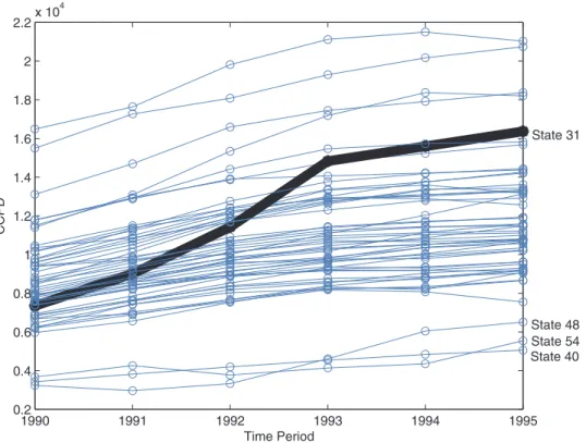
To better understand Step 2, let’s examine the
first graph of Section 4, where hospital claims over a period of six years are plotted for 54 states/regions across the United States. In the plot, we clearly see that all claims within each of the states 40, 48, and 54
are apart from the bulk of other states. They would be treated as between-risk outliers because each of these states affects the level of variability (heterogeneity)
among the states. Procedures that treat these risks the
same way as other risks produce significantly larger estimates of between-risk variability of random effects (i.e., sˆ22
a). N
remark 3 (Mean correction factors)
In view of the mixed linear model as described in Section 7.3, residuals that follow asymmetric log-location-scale distributions have no longer mean zero. Thus, the expectations E(log(yi)) and E(log(yiai))
dif-fer from Xib and li, respectively. Therefore, to ensure
that the estimators are targeting the right variables when estimating li, we need to correct the equation
towards the mean by adding EˆF0(ei). This also explains
the word “corrected” in the acronym CATL. N
2.2. Robust credibility ratemaking
The re-weighted estimates for location, lˆi, and
structural parameters, qˆ
CATL = (sˆ2a1, . . . , sˆ 2
aq, sˆ
2
e), are
used to calculate robust credibility premiums for the ordinary but heavy-tailed claims part of the original data. The robust ordinary net premiums
ˆit ˆ ˆ , , t 1, . . . , 1, = 1, . . . ,i I ordinary
it ordinary
rBLUP i i
(
)
µ = µ α = τ +
are found by computing the empirical limited expected
value (LEV) of the fitted log-location-scale distribu-tion of claims. The percentile levels of the lower bound
ql and the upper bound qg used in LEV computations by the random effect significantly deviates from
the overall portfolio profile. These risks are iden-tified when their robusiden-tified Mahalanobis dis-tance (this is a Wald-type statistic with robustly estimated input variables) exceeds some adaptive cutoff point. The process results in a “cleaned” sample of risks, denoted as
x z y x z y
i I
i i
( )
i i ii ii ii ii(
** **, ,log **,υ**)
, . . .,( ** **τ , τ ,log( )**τ ,υ**τ ),= 1, . . . , *.
1 1 1 1 * * * *
Note that the number of remaining risks is I* (I* ≤ I).
3. CATL estimators.
In the final step, the CATL procedure employs traditional likelihood-based methods, such as (restricted) maximum likelihood, on the cleaned sample and com putes re-weighted parameter esti-mates bˆCATL and qˆCATL= (sˆ2a1, . . . , sˆ
2
aq, sˆ
2
e). Here, the
subscript CATL emphasizes that the maximum likelihood type estimators are not computed on the original sample, i.e., the starting point of Step 1, but rather on the cleaned sample which is the end result of Step 2.
Using the described procedure, we find the shifted
robust best linear unbiased predictor for location:
X Z ( )
λ =ˆi ** ˆi βCATL+ ** ˆi αrBLUP i, +EˆF0 εi , i=1, . . . , ,I
where bˆCATL and aˆrBLUP,i are standard likelihood-based
estimators but computed on the clean sample from Step 2. Also, EˆF0(ei) is the expectation vector of the
t*i -variate cdf Ft*i (0, Rˆi). For symmetric error distri -butions we obtain the special case EˆF0(ei) = 0.
remark 1 (Within-risk outliers)
To illustrate what the above-described procedure
does in Step 1, let’s take a look at the first graph
of Section 3, where a multiple time series plot of
Hachemeister’s bodily injury data is given. Notice
Goovaerts and Hoogstad (1987), Dannenburg, Kaas, and Goovaerts. (1996), Bühlmann and Gisler (1997), Frees, Young, and Luo (1999), Garrido and Pitselis (2000), and Pitselis (2002, 2008) used this data set
to illustrate the effectiveness of diverse regression credibility ratemaking techniques.
3.1. Data characteristics
Hachemeister (1975) considered t= 12 periods, from the third quarter of 1970 to the second quarter of 1973, of claim data for bodily injury that are covered by a private passenger auto insurance. The response variable of interest to the actuary is the severity
aver-age loss per claim, denoted by yit. It is followed over the periods t = 1, . . . , ti= t for each state i = 1, . . . , I.
Average losses were reported from I = 5 different states (Appendix, Section 7.1).
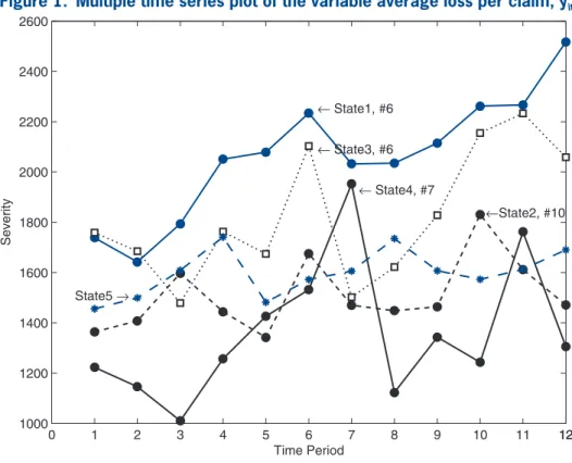
A multiple time series plot of the observed variable average loss per claim, yit, is provided in Figure 1.
The plot indicates that states differ with respect to their within-state variability and severity. State 1 reports the highest average losses per claim, whereas State 4 seems to have larger variability compared to
other states. For all five states we observe a small
increase of severity over time. Since yit varies over states and time (periods t = 1, . . . , 12), these charac-teristics are important explanatory variables. There-fore, Hachemeister originally suggested using the linear trend model given by
x z
yit = β + α + εit it i it, (1)
where p = q = 2 in (5) and xit = zit = (1, t). This
results in a random coefficients model of the form yi = Xi(b + ai) + ei, with diagonal matrix Ri =
Var(yiai) = Var(ei) = se2 diag(u-i11, . . . , u-it1), where uit > 0 are some known (potential) volume
mea-sures. By assumption (b) in Section 7.2, we consider independent (unobservable) risk factors that have variance-covariance structure D = diag(s2
a1, s 2
a2). Notice that the quarterly observations #6 in State 1,
#10 in State 2, #7 in State 4, and maybe #6 in State 3 seem to be apart from their state-specific inflation
trends (see Figure 1).
are usually chosen to be extreme, e.g., 0.1% for ql and 99.9% for qg.
Then, robust regression is employed to price sepa-rately identified excess claims. The risk-specific excess claim amount of insured i at time t is defined by
O
for y q
y q for q y q
q q for y q
it
it ordinary
it l
it l it ordinary
l it g
g l it ordinary it g
(
)
(
)
= −µ− − µ ≤ <
− − µ ≥
ˆ
ˆ , < .
ˆ , .
ˆ , .
Further, let It denote the number of insureds in the portfolio at time t and let T
i I i
= τ
≤ ≤
max ,
1 the maximum
horizon among all risks. For each period t= 1, . . . , T, we find the mean cross-sectional overshot of excess claims Oˆit= I-1
t
Σ
Iti=1Oˆit, and fit robustly the randomeffects model
…
i o
Oˆ =t tξ + εt, t= 1, , ,T
where ot is the row-vector of covariates for the hypothetical mean of overshots x. Here we choose ot= 1, and let xˆ denote a robust estimate of x. Then,
the premium for extraordinary claims, which is com-mon to all risks i, is given by
o it extra
t
µ = ξˆ.
Finally, the portfolio-unbiased robust regression
credibility estimator is defined by
i I
i CATL
rBLUP i i ordinary
rBLUP i i extra
i
(
)
i(
)
iµˆ ,τ +1 αˆ , = µˆ ,τ +1 αˆ , + µˆ ,τ +1, =1, . . . , .
From the actuarial point of view, premiums assigned
to the insured have to be positive. Therefore, we deter-mine pure premiums by max 0, ˆi, 1 ˆ , .
CATL rBLUP i
i
{
µ τ +(
α)
}
3. Hachemeister’s bodily
injury data
variable in the framework of adaptively truncated likelihood credibility. Then, we fit (log-normal) mod-els of the form
x z
ln y
( )
it = β + α + ε = λ + εit it i it it it, (2)where eit~ N(0, s2eit). First of all, we assume that error
terms are serially uncorrelated and process variances are equal for all states, so that s2
ei=s
2
e. This yields
the unweighted covariance matrix Ri = R =s2
e It×t,
i = 1, . . . , I, as special case of (1). Results of the
fitted model using CATL based on Henderson’s
Mixed Model equation (H) are presented in Table 1. In real-data sets where the within-risk variability dif-fers considerably from risk to risk, it is more appro-priate to model unequal process variances when using CATL methods. As noted by Dornheim (2009), this assumption is rather significant for detection of
atypi-cal data points. Figure 1 indicates substantial dif -ferences in within-risk variability among the states. Hence, we fit model (2) twice, once when assum-ing equal (E) process variances and another time for
We use Hachemeister’s regression model (1) as our
reference model to facilitate comparison of CATL cred-ibility with other estimators discussed by the authors mentioned above. We also consider a revised version
of Hachemeister’s model. When applying the linear
trend model to bodily injury data, Hachemeister (1975) obtained unsatisfying model fits due to systematic underestimation of the regression line. Bühlmann and
Gisler (1997) suggest taking the intercept of the regres -sion line centered at the mean time (instead of the ori-gin of the time axis). This ensures that the regression line stays between the individual and collective regres-sion lines. Accordingly, we choose design matrices Xi= (xi1, . . . , xit)′ and Zi= (zi1, . . . , zit)′, with xit= zit=
(1, t - Gi)′, where Gi=u-1
ii
Σ
tt=1tuit, is the center of
grav-ity of the time range in risk i, and uii=
Σ
tt=1uit.
3.2. Model estimation, outlier detection
and model inference
For Hachemeister’s regression credibility model
and its revised version (R), we use ln(yit) as response
0 1 2 3 4 5 6 7 8 9 10 11 1212
1000 1200 1400 1600 1800 2000 2200 2400 2600
← State1, #6
← State4, #7
←State2, #10
← State3, #6
State5 →
Time Period
Severity
it is common to observe situations, where risks with larger exposure measure typically exhibit lower
vari-ability (Kaas, Dannenburg, and Goovaerts 1997; Frees, Young, and Luo 2001). Here, it seems that number of claims per period, denoted by uit, significantly affects
the within-risk variability. Indeed, the data set presented in the appendix supports this fact. In comparison to number of claims, State 4 reports high average losses per claim. This, in turn, yields to the increased
within-state variability that is noticeable in Figure 1.
To obtain homoscedastic error terms, we fit models using uit as subject-specific weights. This model can
be written as
x z
ln y
( )
it = β + α + ε υit it i it it ,1 2
where {eit} is an i.i.d. sequence of normally distrib-uted noise terms. Similarly, the classical linear trend model as described by Hachemeister becomes
x z
yit = β + α + ε υit it i it it .
1 2
In view of the latter regression equation,
Hachemeis-ter’s model can be considered as generalization of the
weighted Bühlmann-Straub model.
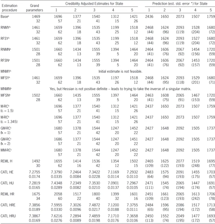
Our findings for fitting of weighted regression models to Hachemeister’s data are shown in Table 2,
together with the results obtained from other prominent estimation procedures. The base model is the linear unequal (U). Here is a summary of all the notations
used in Tables 1–3:
• REML H and REML HR: REML fitting, based
on Henderson’s mixed model equations, of
Hache-meister’s model (REML H) and
Hachemeister’s-revised model (REML HR).
• CATL HE and CATL HU: CATL fitting, based
on Henderson’s mixed model equations, of Hache-meister’s model using the assumption of equal pro -cess variances (CATL HE) and unequal pro-cess variance (CATL HU).
• CATL HRE and CATL HRU: CATL fitting,
based on Henderson’s mixed model equations, of
Hachemeister’s-revised model using the assump
-tion of equal process variances (CATL HRE) and unequal process variance (CATL HRU).
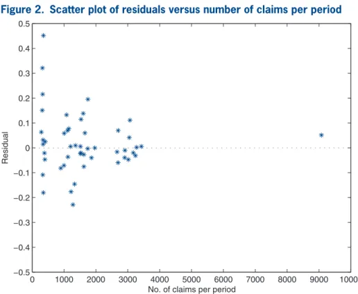
Scenario 1 denotes the real-data set used by Hache-meister. We report fixed effects b (intercept and slope) and for each state credibility adjusted estimates and predicted average claim sizes (premiums for the next period, t = 13). Further, in Figure 2 we plot residuals
from the fitted log-Hachemeister model (2) versus the potential exposure measure, number of claims per
period. The megaphone-shaped picture reveals that the logarithmic transformation of average loss per claim did not remove heteroscedasticity of error components. Thus, additional weighting is required. In practice,
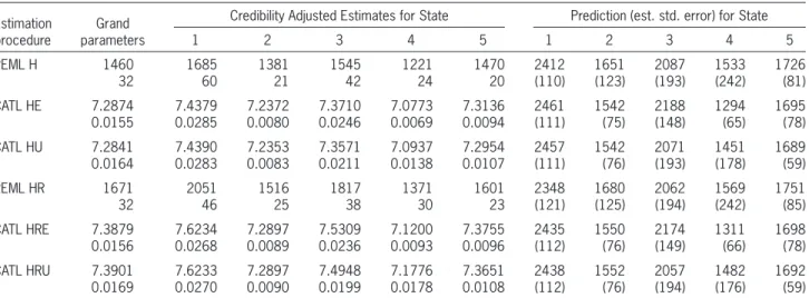
Table 1. Grand parameters, credibility adjusted estimates, and predictions of Hachemeister’s bodily injury data (Scenario 1) based on unweighted regression
Estimation
procedure parametersGrand
Credibility Adjusted Estimates for State Prediction (est. std. error) for State
1 2 3 4 5 1 2 3 4 5
REML H 1460
32 168560 138121 154542 122124 147020 2412(110) 1651(123) 2087(193) 1533(242) 1726(81) CATL HE 7.2874
0.0155 7.43790.0285 7.23720.0080 7.37100.0246 7.07730.0069 0.00947.3136 2461(111) 1542(75) 2188(148) 1294(65) 1695(78) CATL HU 7.2841
0.0164 7.43900.0283 7.23530.0083 7.35710.0211 7.09370.0138 0.01077.2954 2457(111) 1542(76) 2071(193) 1451(178) 1689(59) REML HR 1671
32 205146 151625 181738 137130 160123 2348(121) 1680(125) 2062(194) 1569(242) 1751(85) CATL HRE 7.3879
0.0156 7.62340.0268 7.28970.0089 7.53090.0236 7.12000.0093 0.00967.3755 2435(112) 1550(76) 2174(149) 1311(66) 1698(78) CATL HRU 7.3901
0.0169 7.62330.0270 7.28970.0090 7.49480.0199 7.17760.0178 0.01087.3651 2438(112) 1552(76) 2057(194) 1482(176) 1692(59)
Note: For REML procedures, we report grand mean, bˆ, and corresponding credibility adjusted estimates, bˆi.
• Base: Linear trend model (Goovaerts and Hoogstad 1987).
• RNMY and RNMN: REML fitting; Newton-
Raphson iteration method; Rao’s MIVQUE(0) start -ing values; Estimator of variance-covariance matrix
is constrained to be positive definite = Yes (RNMY) and = No (RNMN). (Frees, Young, and Luo 1999). • RFSY and RFSN: REML fitting; Fisher-Scoring
iteration method; Swamy’s starting values; Estima -tor of variance-covariance matrix is constrained to
be positive definite = Yes (RFSY) and = No (RFSN).
(Frees, Young, and Luo 1999).
• MNMY and MNMN: Maximum likelihood
fit-ting; Newton-Raphson iteration method; Rao’s MIVQUE(0) starting values; Estimator of
variance-covariance matrix is constrained to be positive
definite = Yes (MNMY) and = No (MNMN). (Frees,
Young, and Luo 1999).
• MFSY and MFSN: Maximum likelihood fitting;
Fisher-Scoring iteration method; Swamy’s starting
values; Estimator of variance-covariance matrix is
constrained to be positive definite = Yes (MFSY)
and = No (MFSN). (Frees, Young, and Luo 1999). trend model estimated by Goovaerts and Hoogstad
(1987). To investigate the influence of the pursued procedure for estimation in Hachemeister’s regression model, Frees, Young, and Luo (1999) implemented
several combinations of estimation methods (R =
REML, M = Maximum likelihood), iteration methods (N = Newton-Raphson, F = Fisher-Scoring) and start -ing values (M = Rao’s MIVQUE(0), S = Swamy’s moment estimator) in SAS using the package PROC
MIXED. Moreover, the authors distinguish between constraining the estimator of the variance-covariance matrix D, Dˆ, to be positive definite (Y) or not (N). In
order to limit distorting effects of within-risk outliers
on the assessment of individual’s claim experience, Pitselis (2002) applied MM- and GM-estimators to Hachemeister’s regression model. We denote these approaches by MM-RC and GM-RC, respectively.
As an extension of his joint work about robust
esti-mation in the Bühlmann-Straub model (Garrido and Pitselis 2000), Pitselis (2008) also employs regression
M-estimators (M-RC) that are based on Hampel’s
influence function approach (Hampel et al., 1986).
Here is a summary of all the additional notations:
Figure 2. Scatter plot of residuals versus number of claims per period
0 1000 2000 3000 4000 5000 6000 7000 8000 9000 10000
−0.5 −0.4 −0.3 −0.2 −0.1 0 0.1 0.2 0.3 0.4 0.5
No. of claims per period
Table 2. Grand parameters, credibility adjusted estimates, and predictions of Hachemeister’s bodily injury data (Scenario 1) based on weighted regression
Estimation
procedure parametersGrand
Credibility Adjusted Estimates for State Prediction (est. std. error *) for State
1 2 3 4 5 1 2 3 4 5
Basea 1469 1696 1377 1540 1312 1421 2436 1650 2073 1507 1759
32 57 21 41 15 26
RNMYa 1461 1659 1396 1535 1199 1518 2468 1624 2093 1528 1680
32 62 18 43 25 12 (44) (96) (119) (204) (72)
RFSYa 1461 1659 1396 1535 1199 1518 2468 1624 2093 1527 1680
32 62 18 43 25 12 (44) (96) (119) (204) (72)
RNMNa 1501 1660 1434 1555 1394 1464 2464 1606 2067 1454 1720
28 62 13 39 5 20 (41) (76) (92) (156) (59)
RFSNa 1501 1660 1434 1555 1394 1464 2464 1606 2067 1453 1720
28 62 13 39 5 20 (41) (76) (92) (157) (59)
MNMYa Initial estimate is not feasible.
MFSYa 1461 1659 1396 1535 1197 1518 2468 1624 2093 1529 1680
32 62 18 43 26 12 (44) (95) (118) (201) (71)
MNMNa Yes, but Hessian is not positive definite - leads to trying to take the inverse of a singular matrix.
MFSNa 1502 1660 1435 1555 1397 1464 2463 1608 2065 1467 1720
28 62 13 39 5 20 (41) (75) (91) (153) (59)
M-RCb
(c= 1.5) 169657 137721 154041 131215 142126 2437 1650 2073 1507 1759 M-RCb
(c= 1.345) 169657 137721 154041 131215 142126 2437 1650 2073 1507 1759 GM-RCc
(k= 1) 168057 137821 154442 124720 145222 2427 1648 2092 1505 1737 GM-RCc
(k= 2) 168657 137721 154442 124720 145122 2427 1648 2092 1505 1737
MM-RCc 1680 1378 1544 1247 1452 2427 1648 2092 1505 1737
57 21 42 20 22
REML H 1492 1655 1414 1536 1354 1502 2465 1625 2077 1519 1695
30 62 16 42 12 15 (109) (122) (193) (248) (77)
CATL HE 7.2755 7.3790 7.2464 7.3422 7.1169 7.2932 2483 1575 2091 1455 1703 0.0174 0.0335 0.0084 0.0228 0.0114 0.0110 (64) (94) (193) (175) (57) CATL HU 7.2819 7.4348 7.2349 7.3530 7.0901 7.2967 2471 1545 2065 1447 1691 0.0165 0.0289 0.0082 0.0210 0.0137 0.0105 (111) (74) (194) (174) (57)
REML HR 1675 2058 1517 1800 1399 1601 2451 1661 2065 1613 1706
34 60 22 40 32 16 (109) (123) (193) (242) (78)
CATL HRE 7.3856 7.5955 7.3026 7.4872 7.1200 7.3755 2484 1596 2086 1517 1713 0.0189 0.0330 0.0096 0.0217 0.0188 0.0111 (65) (95) (194) (172) (58) CATL HRU 7.3867 7.6216 7.2894 7.4859 7.1710 7.3658 2450 1552 2049 1477 1693 0.0169 0.0276 0.0089 0.0198 0.0176 0.0106 (113) (74) (195) (172) (57)
Sources:a Frees, Young, and Luo (1999), b Pitselis (2008), c Pitselis (2002).
approaches or robust regression techniques discussed
by Pitselis (2002, 2008). For the second and fourth
state, CATL HE/U determines slightly lower
premi-ums. For instance, for State 4 CATL HU yields, 1447 whereas the base model by Goovaerts and Hoogstad (1987) finds 1507. This can be traced back to the
removal of the suspicious observations #6 and #10 in State 2 and #7 in State 4. Robust methods employed
by Pitselis (2002, 2008) hardly react to these potential
outliers. This is mainly due to the subjectively chosen truncation points c and k, which may be inappropriate (too high). CATL HU also detects claim #4 in State 5 as an outlier and assigns negligible excess premiums (discounts) of -1.47 per risk. For the revised linear
trend model (R) patterns are similar. N
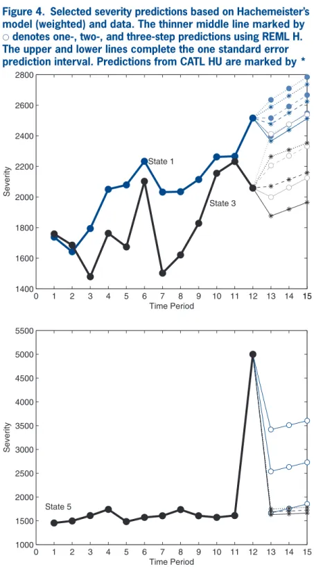
Discussion of Figure 3
We display in Figure 3 the three-step predictions of
the average loss per claim for States 1, 3, and 5 when using REML H and CATL HU. The thinner lines show predictions and one standard error of the prediction for each of the three states. These can be compared
to Frees, Young, and Luo (1999, Figure 1). Note, the
less variable States 1 and 5 have shorter prediction intervals compared to State 3. As expected, in
Sce-nario 1 predictions and intervals obtained from REML and CATL HU nearly coincide. N
To illustrate robustness of regression credibil-ity methods that are based on M-RC, MM-RC, and
GM-RC estimators for quantifying individual’s risk experience, Pitselis (2002, 2008) replaces the last obser -vation of the fifth state 1690 by 5000 (Scenario 2). We follow the same contamination strategy and sum-marize outcomes in Table 3. It turns out that the choice of the methodology has a major impact on the fitting of credibility models.
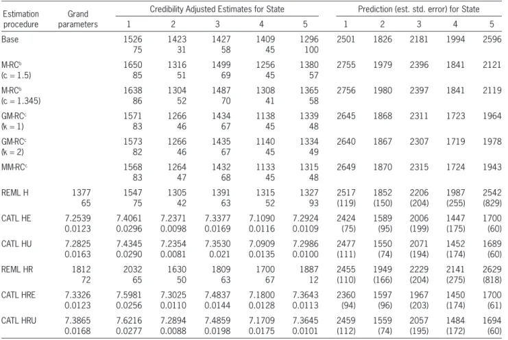
Discussion of Table 3
In the presence of a single outlier in Scenario 2, it is not surprising that standard statistical methods react dramatically. In the contaminated State 5, the REML
H and base credibility estimate of Goovaerts and Hoogstad (1987) get highly attracted by the outlying • M-RC: Robust credibility based on M-estimators.
(Pitselis 2008).
• MM-RC and GM-RC: Robust credibility based on multiple M-estimators (MM-RC) and general-ized M-estimators (GM-RC). (Pitselis 2002).
The reliability of credibility estimates, µˆi,t+1, is of major concern to the insurer. In particular, down-biased predictions result in too-low portfolio premi-ums, which in turn lead to insufficient funding and
threatening of the insurer’s solvency in the long-run.
To assess the quality of assigned credibility premi-ums we also report their standard errors in Table 2. These can be used to construct prediction intervals of
the form BLUP (credibility estimate µˆi,t+1) plus and
minus multiples of the standard error (Frees, Young,
and Luo 1999). Here, we estimate the standard error of prediction, sˆ
µˆ i,t+1, from the data using the common nonparametric estimator
ˆ ˆ ˆ
ˆ ˆ ,
ˆ
2 1 2
1 2 1
1
2
1
1 2
, 1 MSE bias
y y
i i
i it it it it i it it it it t
t
i
i
∑
(
i∑
)
( )
( )
(
)
(
)
σ = µ − µ
= υ ω υ µ − − υ ω υ µ −
µ
− −
= τ
= τ
τ+
where µˆit denotes the credibility estimate obtained from the pursued regression method, uii is the total
number of claims in state i, and wit is the hard-
rejection weight for the observed average loss per claim yit when employing the CATL procedure. For
non-robust REML where no data points are trun-cated, we put wit= 1 as special case.
Discussion of Table 2
Let us start with Hachemeister’s linear trend
model. We observe that REML estimates based on
Henderson’s Mixed Model Equations, REML H, and the resulting predictions mirror findings of Frees, Young, and Luo (1999) who investigated the influence
observation and increase from 1695 to 2542 and
from 1759 to 2596, respectively. Further, it is well
known that the occurrence of outliers distorts the estimation process of variance components and, hence, yields too-low credibility weights. As a con-sequence, credibility adjusted estimates are pulled toward the increased grand mean (most notably the slope component) which results in inflated credibility premiums and prediction intervals across all states. In particular, for REML H the estimated standard error
in State 5 explodes from 77 to 829 due to enhanced
within-risk variability that is caused by the single catastrophic event. Even though only the fifth con-tract is contaminated, the portfolio-unbiased
regres-sion M- and GM-credibility estimators with chosen
tuning parameters c = 1.345 and k = 2, respectively, are significantly distorted. Indeed, these estimators provide protection in the assessment of the individ-ual state experience. However, they reveal a
substan-tial lack of robustness toward single large claims that have adverse effects on the between-risk variability as well. Consequently, the entire estimation process for states that have merely small claims (e.g., see State 2) also becomes distorted. These deficiencies have been removed by CATL estimators. We observe that CATL HU still provides reasonable credibility premiums for all contracts in the portfolio. Both the grand location, lˆ = (7.28, 0.016), the credibility
adjusted estimates, lˆi, the estimated standard errors,
and predictions of expected claims remain stable. We shall emphasize that the latter changes only
margin-ally from 1691 to 1689 in the contaminated State 5.
The CATL HU identifies the single large claim and distributes uniformly an extraordinary premium of 4.33 to all contracts. N
In Figure 4 we visualize the impact of a single out -lier on the premium ratemaking process. When using classical regression techniques such as REML, the
Figure 3. Selected severity predictions based on Hachemeister’s model (weighted) and data. The thinner middle line marked by d denotes one-,
two-, and three-step predictions using REML H. The upper and lower lines complete the one standard error prediction interval. Predictions from the CATL HU procedure are marked by *
0 1 2 3 4 5 6 7 8 9 10 11 12 13 14 1515
1400 1600 1800 2000 2200 2400 2600 2800
← State 1
← State 3
← State 5
Time Period
Table 3. Grand parameters, credibility adjusted estimates, and predictions of Hachemeister’s contaminated bodily injury data based on weighted regression
Estimation
procedure parametersGrand
Credibility Adjusted Estimates for State Prediction (est. std. error) for State
1 2 3 4 5 1 2 3 4 5
Base 1526 1423 1427 1409 1296 2501 1826 2181 1994 2596
75 31 58 45 100
M-RCb 1650 1316 1499 1256 1380 2755 1979 2396 1841 2121
(c= 1.5) 85 51 69 45 57
M-RCb 1638 1304 1487 1308 1365 2756 1980 2397 1841 2119
(c= 1.345) 86 52 70 41 58
GM-RCc 1571 1266 1434 1138 1339 2645 1868 2311 1723 1964
(k= 1) 83 46 67 45 48
GM-RCc 1573 1266 1435 1140 1334 2640 1867 2307 1719 1978
(k= 2) 82 46 67 45 49
MM-RCc 1568 1264 1432 1133 1315 2649 1870 2315 1724 1943
83 47 68 45 48
REML H 1377 1547 1305 1391 1315 1327 2517 1852 2206 1987 2542
65 75 42 63 52 93 (119) (150) (204) (255) (829)
CATL HE 7.2539 7.4061 7.2371 7.3377 7.1090 7.2924 2424 1589 2006 1447 1700 0.0123 0.0296 0.0098 0.0169 0.0116 0.0109 (75) (95) (199) (175) (60) CATL HU 7.2825 7.4345 7.2354 7.3530 7.0909 7.2986 2477 1550 2071 1452 1689 0.0163 0.0290 0.0081 0.021 0.0135 0.0100 (111) (74) (194) (174) (60)
REML HR 1812 2032 1630 1809 1700 1887 2455 1949 2229 2141 2629
72 65 50 63 67 12 (110) (166) (204) (275) (818)
CATL HRE 7.3326 7.5981 7.3025 7.4837 7.1800 7.3643 2360 1597 1967 1450 1700 0.0123 0.0256 0.0110 0.0144 0.0128 0.0113 (94) (96) (203) (174) (61) CATL HRU 7.3865 7.6216 7.2894 7.4859 7.1709 7.3645 2459 1559 2057 1484 1694 0.0168 0.0277 0.0088 0.0198 0.0175 0.0101 (112) (74) (195) (172) (60)
Source:b Pitselis (2008), c Pitselis (2002).
contaminated contract elevates the grand mean of all states, most of all the forecasted credibility pre-mium and its prediction interval in State 5. Clearly, CATL provides robustness for adequate inference in
Hachemeister’s regression model.
4. Medicare data
In this section, we apply CATL procedures to a health care data set that contains Medicare costs for inpatient hospital charges. This real-data set has been
examined by Frees, Young, and Luo (2001) to dem
-onstrate that general mixed linear models can be used to produce credibility estimates of future claims.
4.1. Data characteristics
The underlying health care data set for Figure 5 has
been published by the Health Care Financing Admin
-istration and reports inpatient hospital charges over
t= 6 years, from 1990 to 1995. These charges have been covered by the Medicare program in I = 54 states across the United States, including the District of
Columbia, Virgin Islands, Puerto Rico, and an unspeci -fied category, in addition to the 50 states.
The Medicare program reimburses hospital claims on per-stay basis, hence, the dependent variable is
covered claims per discharge, denoted by CCPD. The multiple time series plot in Figure 5 indicates that there
is rather substantial variability among the states and some variability over the time. Therefore, it is natural to explain the response at least by the regressors state and
time. Frees, Young, and Luo (2001) investigated sev -eral possible explanatory variables through graphical tools and found that the component average hospital
stay per discharge in days, denoted by AVE_DAYS,
More interestingly, the state of New Jersey (State 31)
reveals a notably greater increase of CCPD over the years 1990 to 1993. Frees, Young, and Luo (2001)
identify this outlying growth of medical costs and take it explicitly into account in their model by incorporat-ing a state-specific correction term for the time slope
in New Jersey. Further analysis (e.g., employing scat -ter plots) shows that the second observation of the 54th state is explained by an unusually high hospital
utilization AVE_DAYS. Thus, this data point that has
large distorting effects on classical estimation proce-dures, such as REML, has been manually removed by
0 1 2 3 4 5 6 7 8 9 10 11 12 13 14 1515
1400 1600 1800 2000 2200 2400 2600 2800
State 1
State 3
Time Period
Severity
0 1 2 3 4 5 6 7 8 9 10 11 12 13 14 15
1000 1500 2000 2500 3000 3500 4000 4500 5000 5500
State 5
Time Period
Severity
Figure 4. Selected severity predictions based on Hachemeister’s model (weighted) and data. The thinner middle line marked by
s denotes one-, two-, and three-step predictions using REML H.
we model the serially uncorrelated error terms by the unweighted variance-covariance matrix Ri = s2eIt×t,
where eit ~ N(0, s2e) for all states. This model can be viewed as an extension of Hachemeister’s linear
trend model in Section 3. It is similar to the preferred
mixed linear model in Frees, Young, and Luo (2001),
denoted by Model 6. Note, however, that their model includes an additional special interaction variable to represent the atypical large time slope in State 31 and is given by
1 31
_ ,
(4)
1 2 4
3 1 2
CCPD YEAR State
AVE DAYS YEAR
it t
it i i t it
(
{ })
= β + β + β =
+ β + α + α + ε
where b2+b41 {State = 31} +ai2 can be interpreted as the New Jersey specific total contribution of the
regressor YEAR.
In our analysis, the CATL procedure detects and rejects all suspicious data points that have been
iden-tified by laborious graphical tools in Frees, Young, and
Luo (2001) and, therefore, supersedes the modeling
the authors (see Frees, Young, and Luo 2001, Table 1, Figure 4). In Figure 5 we observe that two other out-lying risks are State 40 and 48. These states report rela
-tively low CCPD over time and, thus, have a distorting
effect on the estimation of between-state variability.
4.2. Model fitting, outlier detection,
prediction
For CATL we fit an error components model of
the form
ln CCPD YEAR AVE DAYS
YEAR
it t it
i i t it
( )= β + β + β
+ α + α + ε
_
, (3)
1 2 3
1 2
where b = (b1, b2, b3)′ is the grand location,
ai= (ai1, ai2)′ are the unobservable random effects, and xit = (1, t, AVE_DAYSit) and zit = (1, t) are the corresponding explanatory variables for i = 1, . . . ,
I= 54 states followed over the periods t = 1, . . . , t= 6.
Frees, Young, and Luo (2001) found that no weighting
by some exposure measure is required to accommo-date potential heteroscedasticity in the data. Therefore,
1990 1991 1992 1993 1994 1995
0.2 0.4 0.6 0.8 1 1.2 1.4 1.6 1.8 2
2.2x 10
4
State 31
State 48
Time Period
CCPD
State 40State 54
the Medicare data set containing all 54 states, whereas the outlying States 31 and 54 have been deleted for
approach 2. Note that our REML estimates do not incorporate the New Jersey-specific time slope. Discussion of Table 4
When the entire data set is considered (approach 1) we observe that the standard method REML 1 gets attracted by the outlying data points and produces estimates of fixed effects that differ significantly from
those of Model 6. For instance, b3 is 348.3 for Model 6 versus 21.9 for REML 1. Also, REML 1 finds the time slope b2= 675.3 for all states. However, the mean slope of the state of New Jersey should be much steeper (b2+b4= 753.1 + 1540.81) as indicated by Model 6
and Figure 7. Once the States 31 and 54 have been
eliminated (REML 2), these standard estimates are com parable to those in Model 6 but still do not account for the extraordinary increase of hospital costs in State 31. As expected, the robust CATL procedure provides protection against catastrophic events and we do not observe any significant differ-ences between the estimates obtained when
employ-ing CATL 1 or CATL 2. Also, Figure 7 shows that
of New Jersey-specific covariates. Results of the detection process using CATL with equal process
variances are visualized in Figure 6. We see that
State 31 (New Jersey) having an extraordinary high
time slope, States 40, 48 and 54 having unusual
low intercepts, and the second observation of the
54th state (though not visible in Figure 6) have
been entirely removed.
In Table 4 we provide results of fitted regression
models based on Equation (4) for Model 6 in Frees, Young, and Luo (2001), and on Equation (3) for the
CATL approaches 1 and 2. Here, approach 1 denotes
1990 1991 1992 1993 1994 1995
0.2 0.4 0.6 0.8 1 1.2 1.4 1.6 1.8 2
2.2x 10
4
Time Period
CCPD
Figure 6. Multiple time series plot of covered claims per discharge (denoted CCPD) over the years 1990 to 1995 after data cleaning
Table 4. Comparisons of diverse fitted regression credibility models
Model
Parameter Estimates of Model Variables Intercept
(b1)
Year (b2)
Year (State = 31) (b4)
AVE_DAYS (b3)
Model 6* 4,827 753.1 1,540.81 348.3
REML 1 7,932.6 675.3 21.9
REML 2 5,447.9 744.5 301.8
CATL 1 8.491 0.081 0.061
CATL 2 8.504 0.081 0.059
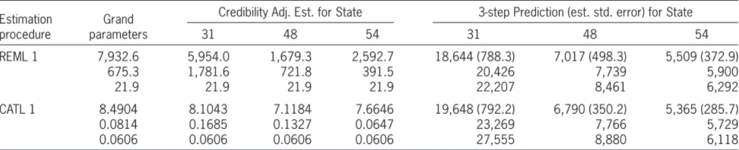
ibility adjusted estimates bˆi when using REML 1.
Likewise, the grand location and credibility-adjusted locations are summarized for CATL 1. The result-ing credibility estimates for the expected CCPDit as well as the estimated standard errors for construc-tion of predicconstruc-tion intervals, are registered over the forecasted periods t = 7, 8, 9, that represent the years 1996 to 1998.
the robust procedures allow for the greater rate of inflation of Medicare costs in New Jersey. N
For the computation of one-, two-, and three-step predictions over the years 1996–1998, we assume
that the most recent subject-specific average
hospi-tal utilizations per discharge (AVE_DAYSit) remain
constant, i.e., AVE_DAYSi6= AVE_DAYSi7. Then, in Table 5 we give the grand mean bˆ and selected
cred-19900 1991 1992 1993 1994 1995 1996 1997 1998
0.5 1 1.5 2 2.5
3x 10
4
New Jersey
Virgin Islands
Other
Time Period
CCPD
Figure 7. The years 1990–1995 represent actual CCPD for selected states New Jersey (State 31), Virgin Islands (State 48), and “Other” (State 54). For 1996–1998, the middle line, marked by s, denotes the one-, two-, and three-step predictions using
REML. The upper and lower lines complete the two standard deviations interval. Predictions and intervals obtained from CATL are marked by d
Table 5. Grand parameters, credibility adjusted estimates, and predictions of Medicare data for selected states New Jersey (State 31), Virgin Islands (State 48) and “Other” (State 54)
Estimation
procedure parametersGrand
Credibility Adj. Est. for State 3-step Prediction (est. std. error) for State
31 48 54 31 48 54
REML 1 7,932.6 675.3 21.9
5,954.0 1,781.6 21.9
1,679.3 721.8 21.9
2,592.7 391.5 21.9
18,644 (788.3) 20,426 22,207
7,017 (498.3) 7,739 8,461
5,509 (372.9) 5,900 6,292 CATL 1 8.4904
0.0814 0.0606
8.1043 0.1685 0.0606
7.1184 0.1327 0.0606
7.6646 0.0647 0.0606
19,648 (792.2) 23,269 27,555
6,790 (350.2) 7,766 8,880
5,365 (285.7) 5,729 6,118
Note: For REML fitting, eq. (4.2), we report grand mean, bˆ, and corresponding credibility adjusted estimates, bˆi.
(PERYPC) and annual percentage growth of
popula-tion (PERPOP) on the response NARSP. The response
variable NARSP represents the MSA’s average sale
price in logarithmic units and is based on transac-tions reported through the Multiple Listing Service, National Association of Realtors. The balanced data set contains I = 36 MSAs with n = 9 annual
observa-tions each, over the years 1986 to 1994. We fit an error
components model of the form
NARSP PERYPC PERPOP
YEAR
it it it
i i it
= µ + β + β
+ β + α + ε ,
1 2
3
where i = 1, . . . , I, t = 1, . . . , ni= n, µ is the popu-lation grand mean, ai is the metropolitan-specific
random intercept and b = (b1, b2, b3)′ is the fixed effects of time-dependent explanatory variables
PERYPCit, PERPOPit, and YEARt, respectively. We assume that the error terms are serially uncorrelated, so that Ri=s2
eiIn×n.
5.1. Data characteristics
In this subsection, we characterize the housing sales price data using graphical and common statistical tools.
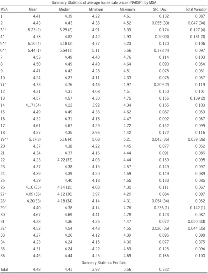
Table 6 summarizes the response variable NARSP, by
MSA. We see that MSAs vary in their average and
median NARSPs. In particular, average sales prices
recorded for metropolitan areas #3, #5, #6 and #19 both start and close at comparatively high price levels. We also observe that the within-MSA variability (Std. Dev.) indicates substantial differences among MSAs.
For instance, we record an extremely high variability
of 0.24 for MSA #29 versus nearly negligible varia-tions of as low as 0.03 for MSA #32. These MSAs are considered to be outlying with respect to their unusually high/low within-MSA variability. These pat terns are highlighted when considering the total
variation of yearly percentage-change in NARSP.
(Note that the total variation of yearly
percentage-change in NARSP is computed as the sum of the eight absolute percentage-changes for each NARSP
observed over a 9-year period.) Discussion of Figure 7
Most of the findings that are outlined in Table 5 for the selected states New Jersey, Virgin Islands, and
“Other” can be visualized in Figure 7. We see that credibility estimates for Virgin Islands and “Other”
are similar. However, we observe that the predic-tion intervals obtained from CATL are somewhat
shorter. For instance, this is due to the removal of the
second data point in the 54th state. Let us focus on predictions in the state of New Jersey. As indicated by results recorded in Table 4, it becomes apparent that REML significantly underestimates the inflation trend of Medicare costs. In contrast, CATL produces
suitable forecasts for CCPDs. We shall also empha
-size that intervals based on CATL are shorter. N
5. Housing prices in
U.S. metropolitan areas
In the case study of this section, we analyze annual housing prices in U.S. metropolitan statistical areas (MSAs). In view of the previous two sections, where Section 3 falls directly in traditional property/casualty field and Section 4 follows the health insurance prac-tice, this type of data is not what actuaries concentrate on currently in their work. With this choice of data we
clearly venture outside the actuary’s comfort zone, but
hope to provide additional insights, highlight the ver-satility of these advanced techniques, and to broaden their area of application.
In this section, we employ graphical tools and sta-tistical criteria to
• view data,
• find atypical data points, and
• evaluate the reliability of the newly designed robust
approach as diagnostic tool.
We also compare fitted parameters of robust CATL with classical REML. The data set we consider is taken
from Frees (2004) and had been studied originally by Green and Malpezzi (2003).
Table 6. Summary statistics of average housing sales prices (NARSP), by MSA. Each MSA has n = 9 observations. The label * (#) marks outlying MSAs identified by using CATL with identically (non-identically) distributed error terms.
For selected criteria the top 4 and the bottom 4 ranks are given in parentheses
Summary Statistics of average house sale prices (NARSP), by MSA
MSA Mean Median Minimum Maximum Std. Dev. Total Variation
1 4.41 4.39 4.22 4.61 0.132 0.087
2 4.43 4.43 4.36 4.52 0.055 (33) 0.047 (34)
3*# 5.23 (2) 5.29 (2) 4.91 5.39 0.174 0.127 (4)
4* 4.73 4.82 4.42 4.93 0.200(3) 0.131 (3)
5*# 5.10 (4) 5.18 (3) 4.77 5.23 0.170 0.106
6*# 5.44 (1) 5.54 (1) 5.11 5.56 0.178 (4) 0.097
7 4.53 4.49 4.40 4.76 0.114 0.103
8 4.50 4.49 4.40 4.64 0.090 0.054
9 4.41 4.42 4.28 4.51 0.078 0.051
10 4.24 4.27 4.11 4.33 0.076 0.057
11* 4.73 4.76 4.46 4.97 0.209 (2) 0.119
12 4.31 4.31 4.08 4.51 0.150 0.101
13 4.57 4.57 4.30 4.75 0.155 0.139 (2)
14 4.17 (34) 4.22 3.92 4.34 0.155 0.103
15 4.49 4.49 4.36 4.62 0.087 0.059
16 4.32 4.31 4.18 4.47 0.092 0.067
17 4.61 4.67 4.29 4.72 0.152 0.099
18 4.27 4.35 3.96 4.42 0.172 0.116
19*# 5.17(3) 5.16 (4) 5.08 5.21 0.043 (35) 0.039 (36)
20 4.37 4.38 4.22 4.45 0.077 0.052
21 4.34 4.37 4.16 4.44 0.091 0.086
22 4.23 4.22 (33) 4.03 4.44 0.159 0.098
23 4.37 4.38 4.15 4.57 0.149 0.097
24 4.39 4.39 4.20 4.59 0.149 0.089
25 4.39 4.40 4.18 4.55 0.133 0.085
26 4.16 (35) 4.14 (35) 4.03 4.30 0.111 0.067
27* 4.09 (36) 4.12 (36) 3.97 4.20 0.084 0.097
28* 4.20(33) 4.18 (34) 4.14 4.31 0.054 (34) 0.052
29* 4.40 4.38 4.14 4.76 0.236 (1) 0.142 (1)
30 4.67 4.69 4.41 4.78 0.123 0.087
31 4.38 4.36 4.26 4.47 0.072 0.050 (33)
32* 4.52 4.54 4.48 4.55 0.026 (36) 0.044 (35)
33 4.27 4.26 4.12 4.39 0.096 0.098
34 4.23 4.24 4.15 4.36 0.077 0.075
35 4.31 4.24 4.22 4.59 0.125 0.094
36 4.45 4.44 4.25 4.69 0.165 0.100
Summary Statistics Portfolio
and 7. We see that not only are overall NARSP increas -ing in time but also that average house sale prices
increase for each MSA. Indeed, as Figure 8 indicates,
there is substantial variability among MSAs, not just a simple time trend. This plot also reveals that MSAs
#3, #5, #6, #19, and #27 stay permanently away from the majority of data, which is seen from unusually
high (low) subject-specific intercepts. Finally, this
preliminary analysis will help us to understand how few atypical MSAs can have disturbing effects on classical estimation of variance components. It turns out that the robust CATL procedure can provide major improvements in model fit over the non-robust REML.
5.2. Model fitting and outlier detection
We find CATL estimates under the following assumptions for residuals: identically distributed, i.e.,
eit ~ N(0, s2e), and non-identically distributed, i.e., eit~ N(0, s2ei). As discussed in a previous section, this
assumption is rather significant for detection of atyp-ical data points. In the current example, the assump-tion of equal error variances allows us to identify such
Table 7 provides summary statistics for NARSP,
by year. We observe that almost all statistical quanti-ties increase over time except for the overall variation (Std. Dev.) in the data. These do not hint at any signifi-cant time-dependency.
Figure 8 is a multiple time series plot of NARSP
and provides a visualization of the findings in Tables 6 Table 7. Summary statistics of average housing sales prices (NARSP), by Year. Each year summarizes I = 36 MSAs. The total summarizes (9 36) 324 observations
Year Mean Median Minimum Maximum Std. Dev.
4.31 4.24 3.92 5.11 0.28
4.36 4.26 3.98 5.21 0.29
4.40 4.32 4.03 5.36 0.33
4.46 4.36 3.98 5.56 0.36
4.50 4.39 3.97 5.56 0.35
4.54 4.45 4.04 5.55 0.34
4.57 4.50 4.12 5.54 0.32
4.60 4.52 4.17 5.52 0.30
4.62 4.56 4.20 5.55 0.29
Total 4.48 4.41 3.92 5.56 0.33
1 2 3 4 5 6 7 8 9
3.8 4 4.2 4.4 4.6 4.8 5 5.2 5.4 5.6 5.8
Time Period
NARSP
Multiple time−series plot of NARSP
MSA
6
3 5 19
27
6. Summary
In this paper, we have illustrated how corrected adaptively truncated likelihood methods, CATL, can be used for robust-efficient fitting of general regression-type models with heavy-tailed data. We have seen that this procedure is a flexible and effec-tive risk-pricing tool. This has been demonstrated through three well-studied examples from the fields of property and casualty insurance, health care, and real estate. In particular, we have shown the entire pro-cess of data analysis, model selection, outlier identi-fication, and the associated statistical inference.
Further, a number of observations can be made based on our analysis. In particular, for Hachemeister’s
bodily injury data, we notice that CATL methods (a) allow to mitigate heteroscedasticity through explicit incorporation of weighting and/or use of logarith-mic transformation; (b) accommodate within-risk vari-ability through modeling of subject-specific process variance; (c) provide high robustness against outliers occurring both within and between risks through adap-tive detection rules that automatically identify and reject excess claims in samples of small size; (d) pro-vide robust credibility premiums; (e) demonstrate efficiency and reliability of detection rules, there-fore making the use of graphical tools (for identifica-tion of outliers) and expert judgment (for the choice of truncation points) non-essential; and (f) compete well against established robust methods. Analysis of the Medicare and the house-pricing data sets just reinforces our findings.
Furthermore, for the readers who are interested in
implementing CATL methods, the matlab computer code is available from the authors upon request. Also, we shall emphasize again that one should be careful about the automatic nature of “data cleaning” and model fitting exhibited by CATL methods (see com-ments c and e above). This aspect of the methodology is an important improvement, as it makes the process of statistical modeling easier and quicker. However, it does not imply that the actuary may now ignore such crucial issues as understanding of the practical MSAs as outlying when their individual within-subject
variation is comparatively high or low. By contrast, when assuming unequal error variances, the CATL procedures only detect those MSAs for which random effects appear to be extreme.
Discussion of Table 8
CATL estimates for the grand mean µˆ are lower than those from REML, which was expected. This effect can be traced back to the identification and
elim-ination of extreme MSAs having rather high NARSP
over time (Table 6). As a result, we record substan-tially reduced estimates for variance components s2
a
and s2
e. In particular, when removing MSAs #3, #4, #5, #6, #11, #19, #27, #28, #29, #32 from the data, the between-MSA variability sˆ2
a drops dramatically
from 0.097 (REML) to as low as 0.018 (CATL, iden
-tical). This is accompanied by a reduction of the over-all within-subject variability sˆ2
e from 0.005 (REML)
to 0.003 (CATL, identical). That is, when assuming identically distributed error terms, the CATL methods eliminate MSAs where either individual random inter-cepts are extreme or their within-subject variability differs clearly from the most typical one. Note that the CATL procedure reliably removes all extraordinary MSAs that have been detected using laborious and
time-consuming graphical tools. For CATL methods
with non-identical error variances the latter type of extremes is ignored, hence fewer MSAs are truncated from the data, and thus, the estimated variance com-ponent sˆ2
a is slightly increased to 0.026. Now, only the
MSAs #3, #5, #6, #19 that have atypical high intercept are marked as extraordinary. We see that the estimates for fixed effects are of the same magnitude. N
Table 8. Fitted values for the housing sales price data
Estimation Procedure
Fixed Effects ComponentsVariance µˆ bˆ1 bˆ2 bˆ3 sˆ2e sˆ2a