CAS: Minimum Bias, Generalized Linear Models, and Credibility in the Context of Predictive Modeling

(1)

Models, and Credibility in the

Context of Predictive Modeling

by Chris Gross and Jon Evans

ABSTRACT

When predictive performance testing, rather than testing model

assumptions, is used for validation, the need for detailed model

specification is greatly reduced. Minimum bias models trade

some degree of statistical independence in data points in exchange

for statistically much more tame distributions underlying

indi-vidual data points. A combination of multiplicative minimum

bias and credibility methods for predictively modeling losses

(pure premiums, claim counts, average severity, etc.) based on

explanatory risk characteristics is defined. Advantages of this

model include grounding in long-standing and conceptually

lucid methods with minimal assumptions. An empirical case

study is presented with comparisons between multiplicative

minimum bias and a typical generalized linear model (GLM).

Comparison is also made with methods of incorporating

cred-ibility into a GLM.

KEYWORDS

(2)

to implement credibility adjustments. Brosius and Feldblum (2003) provide a modern practical guide to minimum bias methods, and Anderson et al. (2007) offer a similar practical guide to GLM. Fu and Wu (2007) demonstrate that a generalized weighting adjustment of minimum bias iteration equations could be used to produce the same numerical estimates as an MLE-estimated GLM with a likelihood function other than Poisson. Note that this paper will use only the standard weighting of multiplicative mini-mum bias iteration equations. A demonstration of predictive model fitting and testing can be found in Evans and Dean (2014), particularly the predic-tive testing methods that will be used in this paper. “Gibbs sampling” is a term we will use for Markov chain Monte Carlo (MCMC) methods as they are implemented using Gibbs sampling software, such as BUGS (Bayesian Inference Using Gibbs Sampling), WinBUGS, or JAGS (Just Another Gibbs Sampler). Scollnik (1996) introduced MCMC. Particularly relevant to this paper is the recent book on predictive modeling for actuaries by Frees, Derrig, and Meyers (2014), which contains very detailed information on GLM, particularly incorporating Gibbs sampling. This paper represents, in a certain sense, an opposite perspective from that of Frees, Derrig, and Meyers (2014) and of Scollnik (1996), by emphasizing very simple models combined with rigorous predictive testing, as described in Evans and Dean (2014). Some more information about the research context of this paper is included in Appendix C.

1.2. Outline

The remaining sections of this paper are as follows:

2. Predictive performance as the modeling objective 3. Multiplicative minimum bias iteration

4. Incorporating credibility

5. Anchoring and iteration blending for practical iterative convergence

6. Testing of individual explanatory variables 7. Empirical case study

1. Introduction

As predictive models that relate losses (pure premiums, claim counts, average severity, etc.) to explanatory risk characteristics become ever more commonplace, some of the practical problems that frequently emerge include the following:

• Models often use complex techniques that are effectively “black boxes” without a lucid concep-tual basis.

• Models may require very detailed parametric or distributional assumptions. Invalid assumptions may result in biased parameters.

• A highly frequentist approach, usually involving maximum likelihood estimation (MLE), can lead to overfitting sparsely populated data bins.

Some long-standing methods can be combined to overcome these problems:

• Minimum bias iterative fitting of parameters is sim-ple, long-standing in practice, and nonparametric in specification.

• Credibility methods are similarly simple and long-standing; moreover, credibility directly solves the sparse bin problem.

Most important, properly done predictive test-ing, in contrast with testing model assumptions, makes highly detailed model specification generally unnecessary.

1.1. Research context

(3)

be fitted to the points (x_i, y_i), i = 1, . . . , k, using any method, and then tested on the points (x_i, y_i),

i = k + 1, . . . , n. The test would be concerned only with how well yˆ_i = mˆxi + bˆ predicts yi for the test set. A bootstrap quintile test might be used, whereby the validation points are sorted by the value yˆ_i into five equal-sized groups. The average value of y_i should ascend with the quintile groups, and for each group the average value of y_i should be close to the average value of yˆ_i.

Figure 2.1 is a hypothetical example of a quintile test, with bootstrap confidence intervals added, as described by Evans and Dean (2014), for the valida-tion of rating factors. Note that the assumpvalida-tion that x∼ normal(0, s2_{) and other implicit assumptions of} linear regression are unnecessary here.

In practice, predictive modelers often split data into three or more sets (i.e., training, testing, and vali-dation), but only the distinction between two separate data sets for fitting and validation will be covered in this paper.

In the predictive framework, detailed model assumptions are not necessary. A model, even if its assumptions seem unjustified or erroneous, is valid as long as it performs well at predicting outcomes for data that were not used to fit its parameters. This 8. Summary discussion

Appendix A. Details of empirical case study Appendix B. Gibbs sampling model code

Appendix C. Response to a reviewer comment about the research context of this paper

2. Predictive performance

as the modeling objective

Traditionally, statistical models tend to use the same data for both fitting and validation. Validation tends to involve testing the model assumptions. For example, a linear regression of the form Y = m X + b + x, where x ∼ normal(0, s2_{), might be fitted, using least squares,} to a set of data points (x_i, y_i), i = 1, . . . , n. Validation tests would check to verify that the residuals xi are normally distributed with constant variance s2_and are independent of x_i, y_i, and each other. Hypothesis tests would then be performed to confirm that the probability is sufficiently remote that the actual data set would result in m = 0 or b = 0 (null hypotheses). This framework relies on detailed assumptions, with-out which validation testing would not be possible.

Modern predictive models split available data into multiple sets for separate fitting and validation. In the previous example, the parameters m and b might

0% 50% 100% 150% 200%

Lowest Low Middle High Highest Lowest Low Middle High Highest

Relative Pure Loss Ratio

Quintiles Based on Expected Rate Relativity

5th Percentile 95th Percentile

Before Rating Factors After Rating Factors

(4)

in each year, as well as when the years are combined. However, this pattern clearly seriously violates many of the previously mentioned standard assumptions for linear regression:

• x is clearly not normal. • s2_{is not constant.} • x is dependent on X.

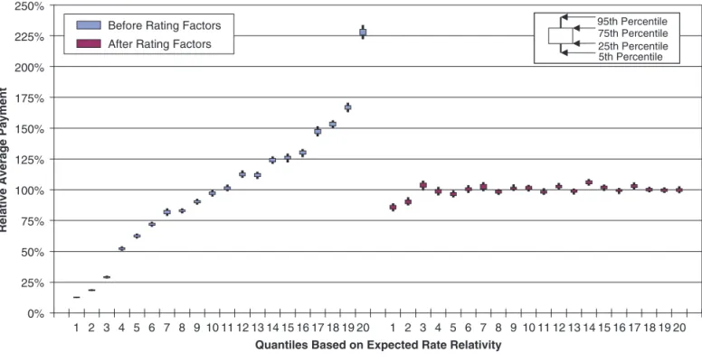
Figure 2.5 shows a bootstrap quintile test using the regression line from Year 1 to predict Year 2. Despite violating the assumptions, predictive perfor-mance for the expected loss rate in Year 2 based on the explanatory variable is excellent, and the model would be very useful in practice.

Figures 2.6 and 2.7 show an alternative compo-sition by Year 1 and Year 2 of the same combined comes with the caveat that care must be taken that

both the fitting and the validation data be represen-tative of—effectively random samples of—the loss process. For example, predictive testing might be misleading if both the fitting data and the validation data occurred in a single year that was influenced by a somewhat rare catastrophe, such as a hurricane.

2.1. A hypothetical example contrasting

predictive performance validation

versus assumption-testing validation

The following hypothetical example illustrates how predictive performance may be high even in a situation where the assumptions of linear regres-sion are seriously violated. Additionally, an alterna-tive situation is shown to illustrate how relying on testing the assumptions of linear regression may lead to missing a high predictive value that might be obtained from a linear regression, or possibly even using a regression estimate that results in very poor predictive performance.

Example 1

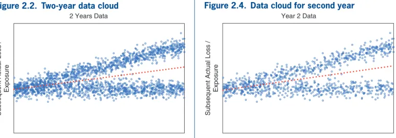
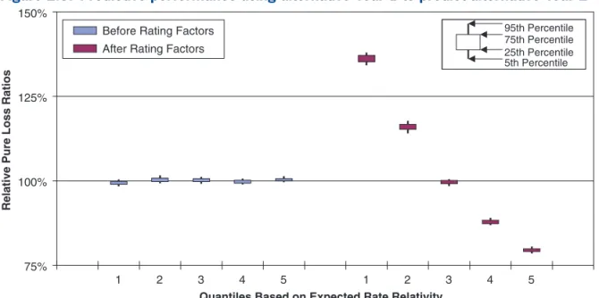
Figure 2.2 displays a data cloud in which the verti-cal axis is the actual loss per exposure subsequent to information available about an explanatory variable shown by the horizontal axis, along with a dotted regression line. Figures 2.3 and 2.4 show the cor-responding data clouds for Year 1 and Year 2, respec-tively. It is clear that the same forked pattern appears

Subsequent Actual Loss /

Exposure

Prior Continuous Explanatory Variable 2 Years Data

Figure 2.2. Two-year data cloud

Exposure

Prior Continuous Explanatory Variable Year 1 Data

Figure 2.3. Data cloud for first year

Exposure

Prior Continuous Explanatory Variable Year 2 Data

(5)

Note that in a real-world application of a predic-tive framework, the performance of the regression line from the first year to predict the second year would be tested. If it performed well, then the regres-sion line for the second year would be used to forecast a third year. So predictive performance testing would result in utilizing the regression line in the first case but discarding it in the alternative case. The real- world loss process would most likely lead to the third year resembling the second year in the first situ-ation, but having a different slope from that of the second year in the alternative situation. Consequently, data shown in Figure 2.2. In this alternative

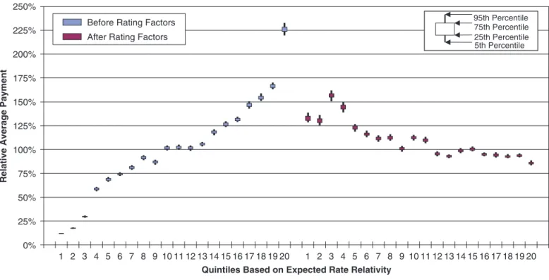
situa-tion, both Year 1 and Year 2 demonstrate patterns that are clearly consistent with the assumptions of linear regression, but the slope has changed signifi-cantly from Alternative Year 1 to Alternative Year 2. Figure 2.8 shows a bootstrap quintile test using the regression line from Alternative Year 1 to predict Alternative Year 2. Despite obeying the linear regres-sion assumptions in each year, the model’s predictive performance is terrible. In fact, it is so bad that it would be much better to simply predict a 0 slope for Alternative Year 2.

5th Percentile 95th Percentile 25th Percentile 75th Percentile 5th Percentile 95th Percentile 25th Percentile 75th Percentile 5th Percentile 95th Percentile 25th Percentile 75th Percentile

75% 100% 125% 150%

1 2 3 4 5 1 2 3 4 5

Relative Pure Loss Ratios

Quantiles Based on Expected Rate Relativity

Figure 2.5. Predictive performance using Year 1 to predict Year 2

Exposure

Prior Continuous Explanatory Variable Alternate Year 1 Data

Figure 2.6. Alternative data cloud for first year

Exposure

Prior Continuous Explanatory Variable Alternate Year 2 Data

(6)

classification dimension. Also, the total exposure in any class is positive,

i kj

∑

=

P_i₁_,..,i_n > 0; otherwise it would

make sense to exclude the class entirely from esti-mating rating parameters. A multiplicative minimum bias model assumes that L_i₁_,..,i_n = Bi1,..,in + Pi1,..,in Xj i

j nj j

, 1,...,

∏

=

.

The parameters X_j,i_j are fitted with the goal of minimiz-ing some bias function, or functions, of the residual errors B_i₁_,..,i_n.

The minimum bias goal is that the sum of the residual errors for each class

i kj

∑

= Bi1,..,in should be 0.

A corresponding iterative sequence of parameter esti-mates can be formed whose convergence corresponds to convergence toward that goal:

1

. , ,1

, , 1

,...,

,..., , ,

1

X

L

P X

j k

j k t

i i i k

l i t l j

n j

l

∑

∏

=

+ =

= ≠

The effective sample is now nj j=

∑

1,...,n

data points with

values i kj

∑

=

Li1,..,in, which reduces to nj

j=

∑

1,...,n

– (n − 1)

linearly independent numbers. There is a correspond-ing (n − 1) dimensional degeneracy in the parameters. predictive performance testing would work well by

obtaining predictive value when it is available but avoiding the pitfall of a poor prediction.

In contrast, in a more traditional statistical frame-work, typically the combined first- and second-year data would be tested for the assumptions of linear regression. The assumption testing would obviously fail, and the regression would be discarded. This would avoid the poor predictive performance in the alternative case but also miss the high predictive value for the first case. However, if it so happened that the assumption testing were performed only on the second-year data in the alternative situation, in which the assumptions would be valid for that year, the regression would be used, resulting in poor pre-dictive performance for the third year.

3. Multiplicative minimum

bias iteration

Suppose the basic data available consist of aggre-gated actual losses L_i₁_,...,i

n ≥ 0 and exposures Pi1,...,in ≥ 0,

(P_i₁_,..,i_n = 0 ⇒ Li1,..,in = 0), where ij = 1, . . . , nj indexes

the individual classes within the classification dimen-sion j, and i₁,..,i_n denotes the cell corresponding to the intersection of a single class selected in each

75% 100% 125% 150%

1 2 3 4 5 1 2 3 4 5

Relative Pure Loss Ratios

(7)

leads to equations for MLE that correspond to a fixed limit point of the minimum bias iteration, as pointed out by Brown (1998).

However, the Poisson distributional assumption is usually unrealistic and not a part of the minimum bias model. Data are generally not restricted to inte-ger values. The Poisson coefficient of variation is not scale independent (e.g., it is 10 times greater when applied to dollar amounts than when applied to the same amounts measured as pennies) and implodes for large nominal means (e.g., a mean of 1 million implies a coefficient of variation of 0.1%). So the Poisson assumption is important only in the optimi-zation equations it implies for MLE.

4. Incorporating credibility

Credibility adjustments, 0 ≤ Z_j,i

j≤ 1, can be easily

and directly incorporated into the iteration equations:

1

1 .

, ,1

, , 1 ,

,..., ,..., , , , ,..., ,..., , , 1 1 1 1 X X Z L P X Z L P X j k

j k t j k

i i i k

l i t l j

j k i i

i i l i t l j n j n j l n n l

∑

∏

∑

∏

(

)

= = + − + = = ≠ ≠

Note that, other than the constraint of the interval [0, 1], nothing has been specified about the deter-mi nation of Z_j,i. There are many possibilities for

Z_j,i_j, including functions of the sum of exposure,

P_j,k = i kj

∑

=

P_i

1,..,in. The ultimate test will be the predictive

performance of the final model regardless of whether

Z_j,i itself satisfies any traditional goals of credibility theory, such as limiting fluctuation or having the greatest accuracy.

For GLM, the basic and common protection against fitting parameters to data that are not credible is to throw away explanatory variables whose parameters are not statistically distinct from 0, those variables with high p-values.

If the parameters X_k,i_k are multiplied by a constant

c> 0 and the parameters X_l,i

l are divided by c, where

0 ≤ k < l ≤ n, then Xj i j nj j

, 1,...,

∏

=

will be unchanged.

The central limit theorem implies that the distri-bution of

i kj

∑

=

L_i₁_,..,i

n can be expected to more closely

resemble a normal distribution, with a generally lower coefficient of variation than the individual cell values

L_i₁_,..,i_n. However, whereas the cellular values L_i₁_,..,i_n can reasonably be assumed to be statistically independent of each other, the further aggregated values

i kj

∑

= Li1,..,in

include many statistical dependencies, since there is an overlap of cells between classes in different dimen-sions. So a trade-off is made for a minimum bias iter-ation model. Statistical independence of sample data points, a desirable property, is partially sacrificed in exchange for the benefit of a more normal distribu-tion, generally having a lower coefficient of variation than the distributions underlying each sample data point. This taming of the distribution of data points means that it becomes less necessary to specify the distribution of the individual cellular loss values or, as may be the case, the distributions of individual loss observations within the cells, as would be necessary for a GLM.

Example 2

Suppose there are three classification dimensions, each with 10 classes, resulting in 1,000 individual cells. We can expect about 100 times as much data volume underlying each class as for each cell, and correspondingly an average coefficient of variation by class that is only about 10% as much as by cell. Two classes in different dimensions overlap in 10 cells, and thus actual losses between them will have a cor-relation coefficient of about 10%.

(8)

of (n − 1) classification dimensions to the value of 1.0, or to fix such a parameter in each of n dimensions and add a single overall base rate parameter. Another approach is to use a single overall base rate and rescale the parameters in each dimension to a weighted aver-age of 1.0 at the end of each iteration.

Example 3

If P = 1 1 1 1



  and L =

1 2 3 4



 , then parameter

iterations will oscillate back and forth between the

values X = 1.5 3.5 2.0 3.0



  and X =

0.6 1.4 0.8 1.2



 .

How-ever, if we anchor one parameter at 1.0, the iterations

will converge to X = 1.000 2.333 1.200 1.800



 .

Iteration blending can be implemented to accel-erate convergence by modifying the iterative equa-tions to be

X Z L P X Z L P X X

j k t

j k

i i i k

l i t l j

j k i i

i i l i t l j

j k t

n j n j l n n l 1 1 ,

, , 1

,

,...,

,..., , ,

, ,...,

,..., , ,

, , 1

1 1 1 1

∑

∏

∑

∏

(

)

( ) = α + −                   + − α

+

=

= ≠

≠

−

where 0 < α < 1 is a selected constant blending parameter.

As an extreme illustration of correlation, let one classification dimension be replicated or made once redundant. Setting α = 0.5 will allow the model to converge. Each one of the replicated dimensions will end up sharing equally in the observed predic-tive relationship, combining together to provide the appropriate prediction. In the case of full credibility, they will exactly reproduce the result obtained from not replicating the dimension. With less than full credibility, the result will not be exactly the same as that obtained from not replicating the dimension, but it will be similar.

To add true credibility, or “shrinkage,” adjustment is complicated. The two main approaches are these:

1. General linear mixed models. At least some rating factors are assumed to be random rather than fixed effects, but an MLE-like fitting method is still used. Numerical solution is rather difficult and, in practice, functions in R or procedures in SAS are used, effectively as black boxes. See Frees, Derrig, and Meyers (2014); Klinker (2001); and Nelder and Verrall (1997) for background.

2. Bayesian networks and Gibbs sampling. Rating factors in each class dimension follow a prior dis-tribution. The parameters of the prior distributions follow distributions that are very diffuse. Numeri-cal solution is performed using a Gibbs sampling program, such as JAGS or WinBUGS. The model itself is elaborately specified and lucid to an audi-ence sophisticated enough read the specification. See Frees, Derrig, and Meyers (2014) and Scollnik (1996) for background.

In Section 7, we will demonstrate an example of the second approach.

5. Anchoring and iteration

blending for practical

iterative convergence

In practice, the convergence of the iterative algo-rithms can be a problem even after the application of credibility. For one thing, there is still the prob-lem of (n − 1) dimensional degeneracy previously mentioned. Also, highly correlated dimensions can contribute to nonconvergence or slow convergence in practice. Other than the automatic degeneracy, we will not attempt to deal in a precise mathematical way with the more general convergence issue, which appears to be an open problem for multiplicative min-imum bias. From a practical point of view, anchoring and iteration blending can effectively provide timely convergence.

(9)

3. Initially we will ignore credibility considerations, aside from reviewing p-values, and later we will use Gibbs sampling to incorporate credibility. 4. The GLM will be fitted, as is customary, to the

individual data records without aggregation into cells based on intersections of the explanatory variables, as happens for the minimum bias model.

7.2. Comparison of GLM and

minimum bias model results

Figures 7.1 and 7.2, and Table 7.1, show the boot-strap quantile testing results of the fitting and the performance testing models. Optimal noise-to-signal estimates along the lines described in Evans and Dean (2014) suggested using 20 quantiles. Also, see Evans and Dean (2014) for details on the definitions of the test statistics. The “old statistic” test measure is the ratio of the variance of the relative average payments after rating factors are applied, to the same variance before rating factors are applied, lower being better. For example, an “old statistic” value of 0.200 can be intuitively interpreted as indicating that the rating factor has eliminated or “flattened out” 80% of the difference in relative losses that it detected. The “new statistic” test measure is essentially the square root of the difference between these two variances, higher being better. For example, a “new statistic” value of 0.300 can be intuitively interpreted as indi-cating that the rating factor has typically reduced the relative differences between quantiles (or, if appli-cable, categories) by 30% (e.g., two cate gories with relative loss ratios of 80% and 130% might have something closer to 90% and 110%, respectively, for relative loss ratios after the rating factor is applied).

Although Figures 7.1 and 7.2 correspond only to the minimum bias fits, Table 7.1 demonstrates that the log-Poisson GLM was identical to the minimum bias approach, and the best-fitting model. In fact, we checked the individual predicted values and verified that they were numerically identical. Log-Gaussian and log-gamma were almost as good. The MLE for our run of log–inverse Gaussian failed to converge, almost certainly driven by its unrealistic variance assumption.

6. Testing of individual

explanatory variables

Sometimes predictive modeling techniques are used specifically to determine whether or not indi-vidual explanatory variables, or equivalent classi-fication dimensions, are statistically significant. As mentioned earlier, when using GLM techniques, it is common to consider the p-values of the estimated parameters. These p-values are calculated under the distributional and other assumptions, such as inde-pendence of the GLM model being used.

Whether distributional assumptions are made (as with GLM) or not (as with minimum bias), tests of predictive performance can be performed and com-pared, with and without a given classification dimen-sion. In cases where the improvement is insignificant, the dimension should be removed for the sake of parsimony.

7. Empirical case study

The empirical data used in this case study consist of 371,123 records of medical malpractice payments obtained from the National Practitioner Data Bank. Three explanatory variables will be used for model-ing payment amounts: Origination Year, Allegation Group, and License Field. The records will be ran-domly split into two sets, for model fitting and vali-dation, respectively. Further details are included in Appendix A.

7.1. GLM model specifications

For our GLM model, we will consider the following:

1. The logarithmic link function, which causes the fit factors to act multiplicatively.

(10)

0% 25% 50% 75% 100% 125% 150% 175% 200% 225% 250%

1 2 3 4 5 6 7 8 9 10 11 12 13 14 15 16 17 18 19 20 1 2 3 4 5 6 7 8 9 10 11 12 13 14 15 16 17 18 19 20

Relative Average Payment

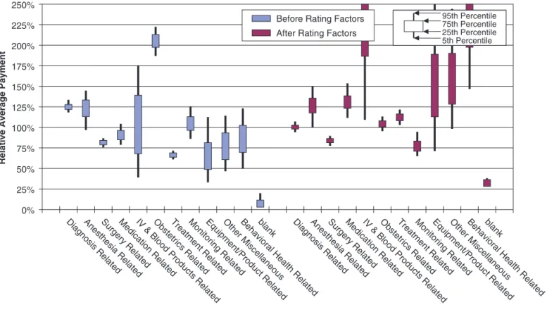
Figure 7.1. Bootstrap 20-quantiles test validation of minimum bias rating factors

0% 25% 50% 75% 100% 125% 150% 175% 200% 225% 250%

blank

Behavioral Health Related Other Miscellaneous Equipment/Product Related Monitoring Related

Treatment Related Obstetrics Related IV & Blood Products Related Medication Related

Surgery Related Anesthesia Related Diagnosis Related blank

Surgery Related Anesthesia Related Diagnosis Related

(11)

independence assumptions, etc. The optimal perfor-mance of minimum bias / log-Poisson is likely due to the general validity of its implicit connection to the central limit theorem, as discussed earlier.

The GLM assumption that all risks are identically distributed is potentially problematic when taken together with the log-link function.

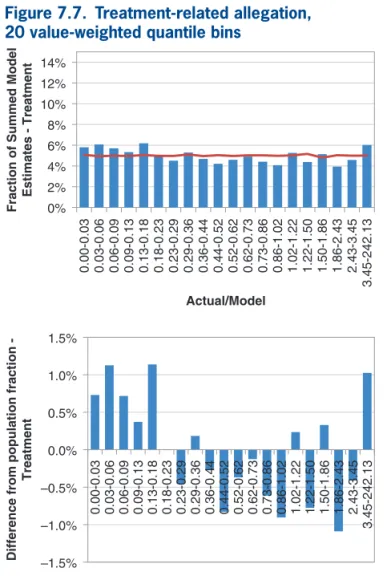
Figures 7.5 through 7.7 illustrate the lack of distri-butional consistency for this data set. We have broken the observations in the training data into 20 quantiles weighted by modeled values, sorted by actual versus modeled result. Using the same breakpoints, deter-mined from the entire training data set, we then calcu-lated the summed modeled values for each allegation group. If the errors were identically distributed for each allegation group, there should be only a random fluc-tuation, around the 5% of total expected for each bin.

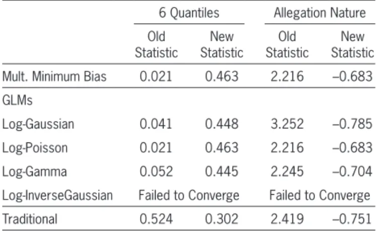
Figure 7.5 shows all allegation groups and, naturally, each bin demonstrates no differences in the weighted proportion. Figure 7.6 shows that the anesthesia-related allegation group has a much higher percentage of the error distribution in the lowest bin than what would be expected from the overall popu-lation. Figure 7.7 shows that, while not as dramatic,

Table 7.1. Predictive performance statistics for various models

20 Quantiles Allegation Nature Old

Statistic StatisticNew StatisticOld StatisticNew

Mult. Minimum Bias 0.007 0.512 0.023 0.425

GLMs

Log-Gaussian 0.010 0.511 0.041 0.422

Log-Poisson 0.007 0.512 0.023 0.425

Log-Gamma 0.009 0.511 0.033 0.422

Log-InverseGaussian Failed to Converge Failed to Converge

Traditional 0.135 0.470 0.089 0.408

0% 25% 50% 75% 100% 125% 150% 175% 200% 225% 250%

1 2 3 4 5 6 7 8 9 10 11 12 13 14 15 16 17 18 19 20 1 2 3 4 5 6 7 8 9 10 11 12 13 14 15 16 17 18 19 20

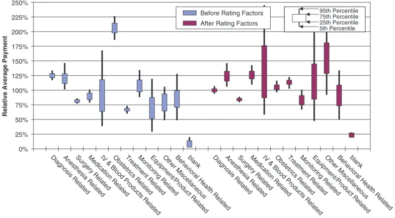
Figure 7.3. Bootstrap 20-quantiles test validation of traditional rating factors

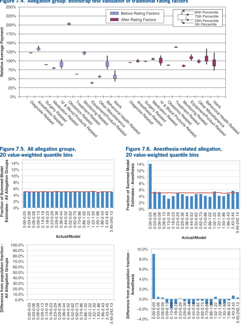
Figures 7.3 and 7.4 correspond to “traditional”

univariate rate relativities for the three explanatory variables. Rating factors are calculated separately and independently in each classification dimension. The traditional method clearly performs much worse than minimum bias and the convergent GLMs, but it is still a great improvement over no adjustment.

(12)

0% 25% 50% 75% 100% 125% 150% 175% 200% 225% 250%

blank

Behavioral Health Relate

d Other Miscellaneous Equipment/Product Related Monitoring Related

Treatment Related Obstetrics Related IV & Blood Products Relate

d Medication Related

Figure 7.4. Allegation group: Bootstrap test validation of traditional rating factors

0% 2% 4% 6% 8% 10% 12% 14%

0.00-0.03 0.03-0.06 0.06-0.09 0.09-0.13 0.13-0.18 0.18-0.23 0.23-0.29 0.29-0.36 0.36-0.44 0.44-0.52 0.52-0.62 0.62-0.73 0.73-0.86 0.86-1.02 1.02-1.22 1.22-1.50 1.50-1.86 1.86-2.43 2.43-3.45

3.45-242.13

Fraction of Summed Model

Estimates - All Allegation Groups

Actual/Model

0.0% 10.0% 20.0% 30.0% 40.0% 50.0% 60.0% 70.0% 80.0% 90.0% 100.0%

0.00-0.03 0.03-0.06 0.06-0.09 0.09-0.13 0.13-0.18 0.18-0.23 0.23-0.29 0.29-0.36 0.36-0.44 0.44-0.52 0.52-0.62 0.62-0.73 0.73-0.86 0.86-1.02 1.02-1.22 1.22-1.50 1.50-1.86 1.86-2.43 2.43-3.45

3.45-242.13

Difference from population fraction

-All -Allegation Groups

Figure 7.5. All allegation groups, 20 value-weighted quantile bins

0% 2% 4% 6% 8% 10% 12% 14%

0.00-0.03 0.03-0.06 0.06-0.09 0.09-0.13 0.13-0.18 0.18-0.23 0.23-0.29 0.29-0.36 0.36-0.44 0.44-0.52 0.52-0.62 0.62-0.73 0.73-0.86 0.86-1.02 1.02-1.22 1.22-1.50 1.50-1.86 1.86-2.43 2.43-3.45

3.45-242.13

Fraction of Summed Model Estimates - Anesthesia

Actual/Model

–4.0% –2.0% 0.0% 2.0% 4.0% 6.0% 8.0% 10.0%

-Anesthesia

0.00-0.03 0.03-0.06 0.06-0.09 0.09-0.13 0.13-0.18 0.18-0.23 0.23-0.29 0.29-0.36 0.36-0.44 0.44-0.52 0.52-0.62 0.62-0.73 0.73-0.86 0.86-1.02 1.02-1.22 1.22-1.50 1.50-1.86 1.86-2.43 2.43-3.45

3.45-242.13

(13)

the treatment-related allegation group shows greater variation than the overall error distribution, with more of the highest and lowest values.

This is far from uncommon with highly skewed insurance data. The problem is compounded by the multiple dimensions of data. Error distributions could be, and likely are, differently distributed across many of the dimensions, if not every dimension being ana-lyzed. Without adjustment, the basic assumption in a GLM is that the errors are identically distributed. The use of the log-link function, in conjunction with maximum likelihood estimation, puts a great deal of faith in the distributional assumption, inferring con-clusions about results in the tail, based on the more voluminous observations at the lower parts of the dis-tribution. But it is the tail itself that is of primary inter-est in most insurance quinter-estions, with the majority of the aggregate losses being caused by the minority of claims. Despite the unreasonable implied assumption of a log-Poisson GLM, because it happens to have effectively the same parameter estimation formulas as the multiplicative minimum bias approach, which has the advantages of the associated central limit theorem (as previously described), it is less vulner-able to these distributional differences.

Table 7.2 shows a comparison of the model biases by allegation group on the validation data using 0.00-0.03 0.03-0.06 0.06-0.09 0.09-0.13 0.13-0.18 0.18-0.23 0.23-0.29 0.29-0.36 0.36-0.44 0.44-0.52 0.52-0.62 0.62-0.73 0.73-0.86 0.86-1.02 1.02-1.22 1.22-1.50 1.50-1.86 1.86-2.43 2.43-3.45

3.45-242.13

Actual/Model

–1.5% –1.0% –0.5% 0.0% 0.5% 1.0% 1.5%

0.00-0.03 0.03-0.06 0.06-0.09 0.09-0.13 0.13-0.18 0.18-0.23 0.23-0.29 0.29-0.36 0.36-0.44 0.44-0.52 0.52-0.62 0.62-0.73 0.73-0.86 0.86-1.02 1.02-1.22 1.22-1.50 1.50-1.86 1.86-2.43 2.43-3.45

3.45-242.13

0% 2% 4% 6% 8% 10% 12% 14%

Fraction of Summed Model Estimates - Treatment

-Treatment

Figure 7.7. Treatment-related allegation, 20 value-weighted quantile bins

Table 7.2. Bootstrapped (actual – modeled)/modeled by allegation group

Multiplicative Minimum Bias Log-Gaussian

Mean 5th % 95th % Mean 5th % 95th %

Diagnosis 1.0% 0.1% 2.0% 1.3% 0.4% 2.3%

Anesthesia 4.3% 0.0% 9.5% 7.1% 2.5% 11.9%

Surgery 0.8% –0.3% 2.1% 1.1% –0.2% 2.5%

Medication 0.9% –2.2% 4.0% 2.2% –0.6% 5.4%

IV & Blood Products 3.0% –11.3% 20.5% 3.6% –6.8% 15.9%

Obstetrics 0.1% –2.4% 2.8% –0.4% –2.3% 1.8%

Treatment –0.5% –2.0% 1.1% –2.5% –4.0% –1.0%

Monitoriing 0.2% –5.1% 6.2% 0.9% –4.3% 5.7%

Equipment/Product –3.4% –11.0% 5.4% 0.0% –9.3% 8.7%

Other –11.1% –15.8% –5.7% –14.3% –19.6% –8.9%

Behavioral Health 11.9% –6.5% 34.4% 13.2% –10.4% 40.9%

(14)

tends only to erode overall predictive value for this large data set, with only truly predictive variables included.

To construct a smaller example in which cred-ibility is more relevant, we will use a random set of only 5,000 records for fitting and another random set of 5,000 records for testing, shown in Tables 7.4 and 7.5, and Figures 7.8 through 7.11. We will also do a full test using all the remaining 366,123 records not used for fitting, shown in Tables 7.6 and 7.7, and Figures 7.12 and 7.13.

As Tables 7.4 through 7.7 and Figures 7.8 through 7.12 show, the incorporation of credibility was particularly important when distinguishing dif-ferences between the allegation groups. Actuaries are regularly asked to provide estimates of the impact of multiplicative minimum bias with full credibility

ver-sus GLM with a log-Gaussian assumption. To do so, it compares actual aggregated results by allegation group with aggregated modeled results over a number of bootstrapped test sets. Despite the log-Gaussian assumption’s better characterizing the distribution of the data than does the log-Poisson assumption, it ultimately produces estimates that are more vulner-able to distributional differences. The only allegation group with a worse log-Gaussian mean bias is that of equipment/product-related payments, and in that group, both sets of bootstrapped ranges contain 0, suggesting that the bias measure is inconclusive.

7.3. Incorporating credibility

into minimum bias

Although the overall predictive performance with-out any credibility adjustments was very good, there are reasons to explore credibility. In some sparsely populated classes for License Field, rating variables might be so unreliable as to lead to adverse selection problems in real-world applications.

In the previous example, the p-values for the rating factors in the log-Poisson were all infinitesimally low (the largest p-value ∼ 10–204_{). This is likely due to the} problematic general phenomenon that p-values always tend to implode with very large volumes of data, such as the volume in the example. In stark contrast, most of the p-values for the log-Gaussian and log-gamma models were high, from 1% to approaching 100%. Whether these p-value results indicate that any of the likelihood selections are valid, or whether they do not, they demonstrate the generally awkward nature of try-ing to use p-values and class consolidation to handle the lack of credibility in sparsely populated classes.

Rather than attempt a p-value-based class consoli-dation, we will explore the impact of a very simple credibility adjustment for minimum bias. We select

the very simple form Z P

P K

j i

j

,

=

+ , where Pj,ij is the

number of records in which the i_j class for classifica-tion dimension j and K ≥ 0 is a judgmental selecclassifica-tion. Table 7.3 shows that this simple credibility adjustment

Table 7.3. Predictive performance statistics for credibility-adjusted multiplicative minimum bias

Statistic StatisticNew StatisticOld StatisticNew Mult. Minimum Bias

K = 0 0.007 0.512 0.023 0.425

K = 1 0.009 0.511 0.032 0.425

K = 10 0.010 0.511 0.030 0.423

K = 25 0.009 0.510 0.029 0.425

K = 50 0.010 0.511 0.022 0.424

K = 100 0.011 0.511 0.028 0.425

K = 200 0.013 0.509 0.031 0.423

K = 700 0.023 0.505 0.082 0.414

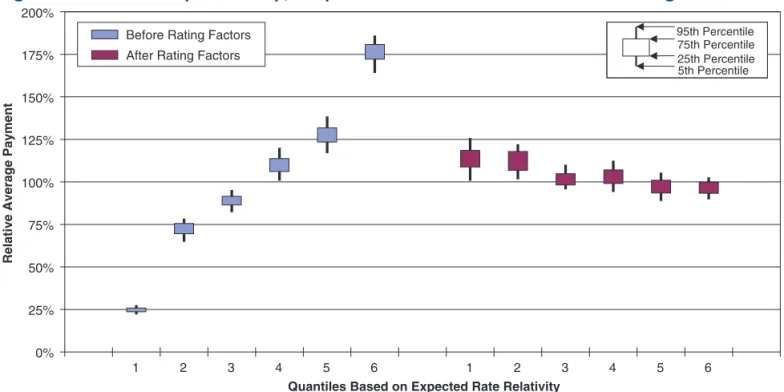
Table 7.4. Smaller-sample predictive performance statistics for various models

Mult. Minimum Bias 0.021 0.463 2.216 –0.683

GLMs

Log-Gaussian 0.041 0.448 3.252 –0.785

Log-Poisson 0.021 0.463 2.216 –0.683

Log-Gamma 0.052 0.445 2.245 –0.704

(15)

U_1,j = 0 j = 1, 2, 3

U_1,4 = Uniform(0, 20)

U_i_,1 ∼ Normal(−s12/2, s12) i = 2, . . . , 83

U_i_,2 ∼ Normal(−s12/2, s12) i = 2, . . . , 12

U_i_,3 ∼ Normal(−s12/2, s12) i = 2, . . . , 9 s12 ∼ Lognormal(0, 10)

s22∼ Lognormal(0, 10)

dk∼ Normal(−s22/2, s22) k = 1, . . . , n

Y_k ∼ Poison(Exp(dk + U1,4 + Ui1,k,1 + Ui2,k,2 + Ui3,k,1))

k = 1, . . . , n

Y_k are the individual actual claim amounts to be fitted. U_i,j are parameters in log space, with U_1,4 being a constant and the other j = 1, 2, or 3, cor-responding to License Field, Allegation Group, and Origination Year, respectively. i_j,k is an index of which class the Y_k observation falls into in each clas-sification dimension. dk is a random overdispersion for each observation, which itself has variance s22. s12 is the parameter variance for each class parameter. Since U_1,4, s12, and s22 follow highly diffuse distri-butions, they will effectively be “fitted” parameters when Gibbs sampling is performed. s12 and s22 conceptually correspond to parameter and process variances in credibility, respectively.

rating variables despite having less than fully cred-ible data. While the overall result may appear to be relatively unaffected by increasing the credibility standard, the ability to differentiate between them more robustly is illustrated.

7.4. Incorporating credibility into GLM

We can incorporate credibility, or “shrinkage” of parameter estimates, into a GLM model by defining a hierarchical Bayesian network of random variables:

Table 7.5. Smaller-sample predictive performance statistics for credibility-adjusted multiplicative minimum bias

K = 0 0.021 0.463 2.216 –0.683

K = 1 0.016 0.457 1.138 –0.419

K = 10 0.012 0.461 0.454 0.246

K = 25 0.022 0.458 0.394 0.316

K = 50 0.043 0.450 0.376 0.338

K = 100 0.068 0.449 0.373 0.345

K = 200 0.093 0.432 0.384 0.345

K = 700 0.255 0.387 0.479 0.319

1 2 3 4 5 6 1 2 3 4 5 6

0% 25% 50% 75% 100% 125% 150% 175% 200%

(16)

0% 25% 50% 75% 100% 125% 150% 175% 200% 225% 250%

blank

25th Percentile 75th Percentile 5th Percentile 95th Percentile

25th Percentile 75th Percentile 5th Percentile 95th Percentile 25th Percentile 75th Percentile

Figure 7.9. Smaller-sample allegation group: Bootstrap test validation of minimum bias rating factors

1 2 3 4 5 6 1 2 3 4 5 6

0% 25% 50% 75% 100% 125% 150% 175% 200%

(17)

0% 25% 50% 75% 100% 125% 150% 175% 200% 225% 250%

blank Behavioral Health Relate

Figure 7.11. Smaller sample, allegation group: Bootstrap test validation of minimum bias (credibility K= 10) rating factors

Table 7.7. Full test of smaller-sample predictive performance statistics for credibility-adjusted multiplicative minimum bias

K = 0 0.031 0.488 1.906 –0.403

K = 1 0.020 0.492 0.835 0.139

K = 10 0.012 0.494 0.169 0.380

K = 25 0.013 0.493 0.187 0.379

K = 50 0.026 0.489 0.215 0.372

K = 100 0.063 0.479 0.246 0.364

K = 200 0.117 0.460 0.289 0.355

K = 700 0.300 0.399 0.427 0.317

Table 7.6. Full test of smaller-sample predictive performance statistics for various models

Mult. Minimum Bias 0.031 0.488 1.906 –0.403

GLMs

Log-Gaussian 0.038 0.482 2.673 –0.556

Log-Poisson 0.031 0.488 1.906 –0.403

Log-Gamma 0.072 0.474 3.256 –0.653

(18)

Figure 7.13. Full test of smaller sample, allegation group: Bootstrap test validation of minimum bias (credibility K= 10) rating factors

0% 25% 50% 75% 100% 125% 150% 175% 200% 225% 250%

blank

1 2 3 4 5 6 7 8 9 10 11 12 13 14 15 16 17 18 19 20 1 2 3 4 5 6 7 8 9 10 11 12 13 14 15 16 17 18 19 20

0% 25% 50% 75% 100% 125% 150% 175% 200%

(19)

and U_i_,3, which is not unreasonable, as none of the cor-responding classes in these dimensions are sparsely populated.

Unfortunately, although there was a credibility-like shrinkage effect, the predictive performance actually deteriorated. Figures 7.14 and 7.15 show the deterio-rating situation when the Gibbs sampling with over-dispersion is included in the large split of the data. Table 7.9 shows the deterioration in test statistics for both the large split and the smaller sample.

There are potential criticisms of the Bayesian network model as we have defined it—for example, anchoring the parameters for the first classes U_1,j = 0 We also defined a simpler form of this model,

elim-inating the overdispersion arising from s12 and s22. Running this simpler model numerically produced the same parameters as the MLE log-Poisson/minimum bias with no credibility adjustment, confirming that our Gibbs sampling model is constructed and coded on the right track up to the point of adding credibility adjustments.

When the model including the dk and s22 was run numerically, we observed a shrinkage effect in the set of parameters. Table 7.8 shows that the range of the U_i_,1 contracted significantly with overdispersion. There was a slight broadening of the ranges for U_i_,2

Table 7.8. Shrinkage effect in range of Gibbs-sampled parameter fits

Ui,1 Ui,2 Ui,3

Min Max Min Max Min Max

Large Split

w/o overdispersion –4.103 0.775 –0.920 0.473 0.000 0.691

w overdispersion –2.173 0.550 –0.975 0.742 –0.040 0.494

Smaller Sample

w/o overdispersion –6.570 2.234 –1.405 0.432 0.000 0.742

w overdispersion –2.033 0.963 –1.992 0.318 –0.069 0.691

1 2 3 4 5 6 7 8 9 10 11 12 13 14 15 16 17 18 19 20 1 2 3 4 5 6 7 8 9 10 11 12 13 14 15 16 17 18 19 20

0% 25% 50% 75% 100% 125% 150% 175% 200%

(20)

capture the impact of overdispersion of the Poisson more directly. In all cases, predictive performance deteriorated further or did not improve. The previ-ously presented multiplicative minimum bias model with incorporated credibility would be vulnerable to similar or more extensive potential criticisms. Yet implementing it went quickly, and it easily produced desirable results.

j = 1, 2, 3; offsetting the prior distributions on param-eters so as to have mean 1 after exponentiation

U_i_,1 ∼ Normal(−s12/2, s12) i = 2, . . . , 83; using the same parameter variance, s12, for all three classifica-tion dimensions; etc. However, the authors experi-mented with a myriad of alterations to the model definition, even going so far as to convert the likeli-hood function into a negative binomial distribution to

0% 25% 50% 75% 100% 125% 150% 175% 200% 225% 250%

blank

Figure 7.15. Full test of smaller sample, allegation group: Bootstrap test validation of Gibbs-sampled rating factors with shrinkage

Table 7.9. Test statistics for Gibbs-sampled rating factors

Quantiles Allegation Nature

Old

Statistic StatisticNew StatisticOld StatisticNew Large Split (20 Quantiles)

w/o overdispersion 0.007 0.512 0.023 0.425

w overdispersion 0.102 0.463 0.219 0.376

Smaller Sample (6 Quantiles)

w/o overdispersion 0.021 0.463 2.216 –0.683

w overdispersion 0.101 0.403 3.616 –0.943

Full Test Smaller Sample (20 Quantiles)

w/o overdispersion 0.031 0.488 1.906 –0.403

(21)

without complete distributional specification, in prac-tice may provide predictive value comparable to or better than that of a far more complex model, such as a typical GLM or, particularly, a GLM adjusted to incorporate credibility.

GLM models are fitted to individual data points and require specification of the distributions under-lying each data point. Consequently, GLM models can be significantly vulnerable to inaccurate specifi-cations, and their fundamental complexity makes the practical incorporation of credibility adjustments, such as including random effects or fitting param-eters through Gibbs sampling, very complex.

Philosophically, simpler modeling is desirable. In practice, simpler models are beneficial in many ways, such as lower skill requirements for operational personnel and greater lucidity to a much wider audi-ence. Some previous papers, such as those by Brown (1998) and Mildenhall (1999), have highlighted the sense in which minimum bias iteration is a special case of GLM and encouraged—at least implicitly— minimum bias practitioners to switch to GLM as a richer framework. There is some irony that with the advent of the predictive framework, minimum bias may often be somewhat more advantageous, in prin-ciple and practice. However, it should be emphasized that this does not mean that the detailed specifica-tions of a particular GLM might not produce superior predictive performance in a situation where the pro-cess underlying the data closely matches the particular assumptions of that GLM.

While GLM models are powerful and belong in the set of tools applied by actuaries, consideration should also be given to multiplicative minimum bias models and the traditional actuarial concept of partial cred-ibility. Ultimately the test of any predictive model should be how it performs on out-of-sample data.

Acknowledgments

The authors are thankful to Jose Couret, Louise Francis, Chris Laws, and Frank Schmid for answer-ing some questions that arose in the course of writanswer-ing this paper.

This failed modeling experience in no way proves that a well-performing Gibbs-sampled Bayesian model cannot be defined in this context. Obviously, well-performing examples for much simpler situa-tions, such as one classification dimension and an identity link function, are well known and easy to construct. Nor is the point that the theory behind these models does not provide deep insights into under-standing modeling and statistical estimation. How-ever, in this case, orders of magnitude more input of resources, both in time and sophistication of effort, than was used for minimum bias produced inferior predictive performance. Though neither author of this paper is a specialist in Gibbs sampling methods, one author (Evans) has used them occasionally for over 10 years and informally consulted several specialists with more experience (in Acknowledgments). As of this writing, we have not been able to diagnose why the model as defined performs so much more poorly than a regular MLE GLM with no shrinkage effect. Whether the model is in some way poorly designed or, much less likely, one of the many technical choices made in running the Gibbs sampling software should be tuned differently does not alter the key conclu-sion, namely, that the tremendous additional resource and intellectual burdens of such detailed and sophis-ticated models may offer no advantage, or may even be disadvantageous, in many practical situations of predictive modeling.

8. Summary discussion

(22)

Three explanatory variables were used for model-ing payment amounts: Origination Year, Allegation Group, and License Field. Tables A.1 through A.3 display record counts by each of the explanatory variables overall and for the individual predictive modeling splits.

Appendix A. Details of empirical

case study

The empirical data used in this case study consist of 371,123 records of medical malpractice payments obtained from the National Practitioner Data Bank.

Table A.1. Counts of records by license field

Large Split Smaller Sample

License Field Total Fit Test 5,000 Fit 5,000 Test Full Test

Allopathic Physician (MD) 271,443 135,514 135,929 3,644 3,661 267,799

Phys. Intern/Resident (MD) 2,113 1,063 1,050 34 28 2,079

Osteopathic Physician (DO) 17,612 8,829 8,783 237 244 17,375

Osteo. Phys. Intern/Resident (DO) 324 161 163 8 6 316

Dentist 46,516 23,425 23,091 623 596 45,893

Dental Resident 145 64 81 4 3 141

Pharmacist 1,890 952 938 24 20 1,866

Pharmacy Intern [available 9/9/2002] 2 1 1 0 0 2

Pharmacist, Nuclear 6 4 2 0 0 6

Pharmacy Assistant 19 12 7 0 0 19

Pharmacy Technician [available 9/9/2002] 12 7 5 0 1 12

Registered (RN) Nurse 5,715 2,885 2,830 91 80 5,624

Nurse Anesthetist 1,568 777 791 19 19 1,549

Nurse Midwife 873 431 442 18 8 855

Nurse Practitioner 1,288 598 690 19 24 1,269

Doctor of Nursing Practice [available 11/8/2010] 1 — 1 0 0 1

Advanced Nurse Practitioner [3/5/02 - 9/9/02] 4 3 1 0 0 4

LPN or Vocational Nurse 692 345 347 9 9 683

Clinical Nurse Specialist [available 9/9/02] 18 12 6 1 0 17

Certified Nurse Aide/Nursing Assistant [available 10/17/05] 36 18 18 0 1 36

Nurses Aide 78 39 39 2 2 76

Home Health Aide (Homemaker) 22 10 12 0 0 22

Health Care Aide/Direct Care Worker [available 10/17/05] 3 1 2 0 0 3

Psychiatric Technician 15 10 5 0 0 15

Dietician 22 11 11 0 1 22

Nutritionist 1 1 — 0 0 1

EMT, Basic 200 106 94 3 2 197

EMT, Cardiac/Critical Care 28 17 11 0 0 28

EMT, Intermediate 26 13 13 1 2 25

EMT, Paramedic 59 32 27 0 1 59

Clinical Social Worker 206 107 99 2 0 204

Podiatrist 7,654 3,809 3,845 92 113 7,562

Clinical Psychologist [last use 9/9/02] 875 436 439 15 15 860

(23)

School Psychologist [available 9/9/02] 1 — 1 0 0 1

Audiologist 39 23 16 2 1 37

Art/Recreation Therapist 2 1 1 0 0 2

Massage Therapist 82 54 28 3 1 79

Occupational Therapist 85 43 42 0 0 85

Occup. Therapy Assistant 11 7 4 0 0 11

Physical Therapist 1,094 545 549 14 14 1,080

Phys. Therapy Assistant 94 48 46 0 3 94

Rehabilitation Therapist 9 3 6 0 0 9

Speech/Language Pathologist 14 9 5 0 0 14

Hearing Aid/Instrument Specialist [available 10/17/05] 2 1 1 0 0 2

Medical Technologist [changed to 501(6/15/09)] 64 28 36 0 0 64

Medical/Clinical Lab Technologist [available 6/15/09] 1 1 — 0 0 1

Medical/Clinical Lab Technician [available 6/15/09] 2 — 2 0 0 2

Surgical Technologist [available 6/15/09] 7 4 3 0 0 7

Surgical Assistant [available 6/15/09] 1 — 1 0 0 1

Cytotechnologist [available 11/22/99] 11 7 4 0 0 11

Nuclear Med. Technologist 14 5 9 0 0 14

Rad. Therapy Technologist 12 5 7 0 0 12

Radiologic Technologist 169 89 80 1 0 168

X-Ray Technician or Operator [available 6/15/09] 5 2 3 0 0 5

Acupuncturist 58 22 36 0 0 58

Athletic Trainer [available 11/22/99] 6 3 3 1 0 5

Chiropractor 5,834 2,928 2,906 78 87 5,756

Dental Assistant 15 8 7 1 1 14

Dental Hygienist 41 22 19 1 2 40

Denturist 27 8 19 0 0 27

Homeopath 6 5 1 1 0 5

Medical Assistant 33 14 19 1 0 32

Counselor, Mental Health 167 84 83 1 2 166

Midwife, Lay (Non-Nurse) 22 14 8 0 0 22

Naturopath 17 9 8 0 0 17

Ocularist 25 12 13 0 1 25

Optician 17 10 7 0 0 17

Optometrist 715 367 348 6 11 709

Orthotics/Prosthetics Fitter 9 5 4 1 0 8

Phys. Asst., Allopathic 1,713 847 866 26 22 1,687

Phys. Asst., Osteopathic 137 71 66 3 3 134

Perfusionist [available 11/22/99] 8 2 6 1 0 7

Podiatric Assistant 14 9 5 0 0 14

Table A.1. Counts of records by license field (continued)

(24)

Prof. Counselor 209 109 100 4 3 205

Prof. Cnslr., Alcohol 9 2 7 0 1 9

Prof. Cnslr., Family/Marriage 177 96 81 4 5 173

Prof. Cnslr, Substance Abuse 23 13 10 0 0 23

Marriage and Family Therapist [available 9/9/02] 27 15 12 1 0 26

Respiratory Therapist 48 24 24 1 0 47

Resp. Therapy Technician 14 4 10 0 0 14

Other Health Care Pract, Not Classified [available 11/22/99] 45 31 14 0 0 45

Unspecified or Unknown 170 86 84 1 2 169

Total 371,123 185,562 185,561 5,000 5,000 366,123

Table A.1. Counts of records by license field (continued)

Table A.2. Counts of records by allegation group

Allegation Nature Total Fit Test 5,000 Fit 5,000 Test Full Test

Diagnosis Related 105,674 52,516 53,158 1,409 1,388 104,265

Anesthesia Related 10,974 5,421 5,553 127 153 10,847

Surgery Related 88,763 44,538 44,225 1,176 1,211 87,587

Medication Related 20,197 10,047 10,150 259 268 19,938

IV & Blood Products Related 1,259 625 634 14 16 1,245

Obstetrics Related 25,988 13,081 12,907 384 345 25,604

Treatment Related 100,666 50,517 50,149 1,380 1,372 99,286

Monitoring Related 7,313 3,594 3,719 103 106 7,210

Equipment/Product Related 2,037 989 1,048 32 24 2,005

Other Miscellaneous 7,404 3,791 3,613 106 106 7,298

Behavioral Health Related 677 361 316 7 9 670

blank 171 82 89 3 2 168

Total 371,123 185,562 185,561 5,000 5,000 366,123

Table A.3. Counts of records by origination year

Origination Year Total Fit Test 5,000 Fit 5,000 Test Full Test

1990–1992 40,574 20,306 20,268 568 515 40,006

1993–1994 39,016 19,480 19,536 570 529 38,446

1995–1996 37,048 18,557 18,491 516 509 36,532

1997–1998 35,689 17,838 17,851 490 493 35,199

1999–2000 38,036 19,045 18,991 469 516 37,567

2001–2002 39,277 19,650 19,627 491 533 38,786

2003–2004 36,565 18,256 18,309 472 508 36,093

2005–2007 47,519 23,756 23,763 659 646 46,860

2008–2012 57,399 28,674 28,725 765 751 56,634

(25)

Appendix C. Response to a

reviewer comment about the

research context of this paper

The following question by a reviewer of this paper and the authors’ response may help readers under-stand the research context of the paper.

Reviewer Comment:

Having reviewed this paper and the referenced papers, my sense is that the paper is not present-ing a novel method or novel comparison, but rather providing a case study as a reason for preferring the minimum bias model (optionally with credibility) to a Bayesian method of incorporating credibility con-cerns. If I have misunderstood the authors’ intent in this matter, then the remainder of my review may be a little off.

Authors’ Response:

The reviewer correctly understands that we do use a case study, and other points of discussion, to argue, with particular emphasis on practical considerations, that a credibility-adjusted minimum bias model may be preferable to a Bayesian method of adjusting a GLM in some situations. However, the paper involves much more than that. Also, we view the content of the paper as being significantly novel in several respects that are either completely absent or minimally treated in Casualty Actuarial Society (CAS) and other actu-arial literature:

1. The paper emphasizes the importance of predictive

performance testing rather than assumption test-ing for model validation. This is a general point, but minimum bias is a specific example of a model less specified than GLM that nevertheless may be preferable when predictive performance valida-tion is implemented. Note that we have added an extensive example in a new Section 2.1 that deals with this point.

2. The paper also highlights that although

multi-plicative minimum bias happens to correspond to log-Poisson GLM regarding numerical estimates, it can be justified by a much simpler and less

Appendix B. Gibbs sampling

model code

With Poisson overdispersion

model {

U[1,4]∼dunif(0,20) U[1,1]<-0

U[1,2]<-0 U[1,3]<-0

Tau[1] ∼ dlnorm(0,0.1) Mu<- -pow(Tau[1],-1)/2 Tau[2] ∼ dlnorm(0,0.1) Mu2<- -pow(Tau[2],-1)/2 Tau[3]<-Tau[1]/Tau[2]

for(i in 2:N1) { U[i,1]∼dnorm(Mu,Tau[1]) } for(i in 2:N2) { U[i,2]∼dnorm(Mu,Tau[1]) } for(i in 2:N3) { U[i,3]∼dnorm(Mu,Tau[1]) } for(i in 1:N) {

ProcError[i]∼dnorm(Mu2,Tau[2])

lambda1[i]<-exp(min(20,ProcError[i]+U[1,4]+ U[X[i,1],1]+U[X[i,2],2]+U[X[i,3],3])) Y[i]∼dpois(lambda1[i])

} }

Without Poisson overdispersion

model {

U[1,4]∼dunif(0,20) U[1,1]<-0

U[1,2]<-0 U[1,3]<-0

Tau[1] ∼ dlnorm(0,0.1) Mu<- -pow(Tau[1],-1)/2

for(i in 2:N1) { U[i,1]∼dnorm(Mu,Tau[1]) } for(i in 2:N2) { U[i,2]∼dnorm(Mu,Tau[1]) } for(i in 2:N3) { U[i,3]∼dnorm(Mu,Tau[1]) } for(i in 1:N) {

lambda1[i]<-exp(min(20,U[1,4]+U[X[i,1],1]+ U[X[i,2],2]+U[X[i,3],3]))

Y[i]∼dpois(lambda1[i]) }

(26)

References

Anderson, D., S. Feldblum, C. Modlin, D. Schirmacher, E. Schirmacher, and N. Thandi, A Practitioner’s Guide to Generalized Linear Models (3rd ed.), Arlington, VA: Towers Watson, 2007.

Bailey, R. A., “Insurance Rates with Minimum Bias,” Proceed-ings of Casualty Actuarial Society 50, 1963, pp. 4–13. Bailey, R. A. and L. J. Simon, “Two Studies in Automobile

Insurance Ratemaking,” Proceedings of Casualty Actuarial Society 47, 1960, pp. 1–19.

Brosius, E., and S. Feldblum, “The Minimum Bias Procedure: A Practitioner’s Guide,” Proceedings of Casualty Actuarial Society 90, 2003, pp. 196–273.

Brown, R. L., “Minimum Bias with Generalized Linear Models,” Proceedings of Casualty Actuarial Society 75, 1988, 187–217. Evans, J., and C. Dean, “The Optimal Number of Quantiles for

Predictive Performance Testing of the NCCI Experience Rating Plan,” Variance 8:2, 2014, pp. 89–104.

Frees, E., R. A. Derrig, and G. Meyers, Predictive Modeling Applications in Actuarial Science: Volume 1, Predictive Modeling Techniques, New York: Cambridge University Press, 2014.

Fu, L., and C. P. Wu, “General Iteration Algorithm for Classifi-cation Ratemaking,” Variance 1:2, 2007, pp. 193–213. Klinker, F., “Generalized Linear Mixed Models for Ratemaking:

A Means of Introducing Credibility into a Generalized Linear Model Setting,” Casualty Actuarial Society Forum 2, 2001, pp. 1–25.

Klugman, S., H. H. Panjer, and G. E. Willmot, Loss Models: From Data to Decisions (4th ed.), Hoboken, NJ: Wiley, 2012. Mildenhall, S., “Minimum Bias and Generalized Linear

Models,” Proceedings of Casualty Actuarial Society 76, 1999, pp. 393–487.

Nelder, J., and R. Verrall, “Credibility Theory and Generalized Linear Models,” ASTIN Bulletin 27:1, 1997, pp. 71–82. Scollnik, D., “An Introduction to Markov Chain Monte Carlo

Methods and Their Actuarial Applications,” Proceedings of Casualty Actuarial Society 83, 1996, pp. 114–165.

Venter, G. G., “Discussion of Minimum Bias with Generalized Linear Models,” Proceedings of Casualty Actuarial Society 77, 1990, pp. 337–349.

spec ified argument. That is to say, it can be justi-fied in terms of a basic trade-off that sacrifices some degree of sample independence for greater sample volume to benefit from the central limit theorem.

3. We are not aware of any significant treatment of

credibility-adjusted minimum bias models in CAS or other actuarial literature, but only some brief mention of the possibility of employing credibility adjustments.

4. Additionally, although there has been some

treatment of mixed-effects GLM (or GLMM) in the literature to handle the credibility problem, we believe there has been little treatment of the application of Bayesian methods (such as Gibbs sampling) to the credibility problems with GLM. Applications of Gibbs sampling to GLM have been focused more on determining estimates similar to those from MLE but with additional information on uncertainty in parameter estimates, rather than actual credibility adjustment of estimates.

5. Previous literature on minimum bias models has

limited the number of factors (sometimes referred to as “classification dimensions” or “parameters”) to at most three. In contrast, our paper defines minimum bias models for arbitrarily many fac-tors (“classification dimensions”) so as to make a direct comparison with GLM, which allows an arbitrary number of factors.

6. Compounding this, to the best of our knowledge,