On the Normalized Herfindahl-Hirschman Index: A Technical Note

Available online at www.centmapress.org

Int. J. Food System Dynamics 7 (4), 2016, 382-386

On the Normalized Herfindahl-Hirschman Index:

A Technical

Note

Daniel Cracau and José E. Durán Lima

Economic Commission for Latin America and the Caribbean (ECLAC) in Santiago de Chile, Integration Unit of the International Trade and Integration Division of ECLAC in Santiago de Chile, [email protected]; [email protected].

Received October 2015, accepted July 2016, available online August 2016

ABSTRACT

We compare the application of two different normalization procedures for the Herfindahl-Hirschman Index. We show that structural differences exist between the two indices and derive the conditions for which these differences are more or less substantial

Keywords. Herfindahl-Hirschman Index, normalization JEL Classification: C43, C18

*

Disclaimer: The opinions expressed in this article are those of the authors and do not necessarily reflect the views of ECLAC.

1

Introduction

The so-called Herfindahl-Hirschman Index (HHI), named after its first inventor Hirschman (1945) and its reinventor Herfindhal (1950), was originally used to analyze a country’s trade measuring the concentration in its export or import pattern in a given period of a time. Its well-known definition follows

, (1)

where represents total exports of the economy at hand, represents the share in total exports (or imports, respectively) of product or industry , and is the corresponding number of products or industries. By its nature, , i.e. the original is equal to if the trade pattern is completely concentrated and if all products or industries incur exactly equal shares in exports (or imports, respectively). Thus, the number of relevant items substantially affects the possible range of the

.

When comparing the trade patterns of an economy over the course of time or between several economies, it is likely that the underlying changes. To maintain (or rather create) comparability, one can apply a normalization procedure that redefines the range of the such that it is zero for the case of equal distribution of shares between all items, i.e. for minimum concentration. The common procedure to derive the normalized index, denoted as , is given by

(2)

It is easy to see that the remains if the original is equal to , but becomes if the original index is , that is, minimal.

Baumann (2009) has proposed an alternative normalization approach, which we denote by that follows

. (3)

This procedure also has the property of rescaling the original to values between and . However, it obviously differs structurally from the common normalization. As this alternative normalization measure of Baumann (2009) has been recently appeared in economic analyses (de Pablo et al., 20 14; de Pablo Valenciano, Giacinti Battistuzzi and Garcia Azcaráte, 2015), we will clarify the differences in both approaches thereby hinting on the appropriate use of a normalization measure.

2

Comparison of the two normalization approaches

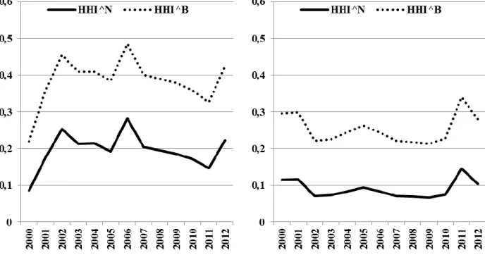
We start our comparison with a practical example derived from D’Elía and Durán Lima (2014). Figure 1 displays the export concentration calculated for Honduras in the period 2000 – 2012, measured by products (Sub-figure 1a) and by destinations (Sub-figure 1b).* When we compare the graphical representation in both sub-figures, we see that the two normalization approaches differ mainly in their absolute level. The is always higher than its counterpart, the . However, looking at their development over time, we find no great differences. Both curves show various movements upwards and downwards in the considered period – both in concentration measured by products as well as by destinations – but are always well aligned. From this practical example, we can derive that for the purpose

*

of the comparison of its development over time, the two normalization approaches seem equally applicable. The question remains to what extent this similarity of both normalized indices is specific to the chosen case of Honduras (where, for example, the number of considered items is quite high in both dimensions: for products and for destinations).

(1a): products (1b): destination

Source: own compilation based on D’Elía and Durán Lima (2014). Figure 1. Export concentration of Honduras, 2000 – 2012

For a detailed analytical comparison of the two normalization approaches, we define their absolute difference as which yields

.† (4)

We obtain the maximum difference through

FOC I: and FOC II : and calculate

FOC I: (5)

FOC II: (6)

†

It can be shown that the first term is always greater or equal to the second term, because . Thus, the bars indicating the absolute value can be dropped.

Using FOC I FOC II, we obtain the condition for the global extreme value as

. (7)

As Equation (7) yields no global extreme value in the defined space ( , we focus on the FOC I in Equation (5), only looking at the limit cases and . For the first case of only one item ( ), we simply get . Here, both normalized indices yield as well and the difference between them is minimized ( ). More interesting is the limit case of an infinite number of items, i.e. . We can derive

. (8)

Indeed, we find that for and , . Because

, we can conclude that this candidate is a maximum.‡ It follows, that for

these conditions, we obtain a maximum difference between the two normalized indices of

. (9)

Result 1. The maximum difference between the two normalized indices of the equals . It appears, when the original is equal to and the number of items approaches infinity.

(2a): absolute (2b): relative

Source: own compilation using MS Excel.

Figure 2. Differences between and (Horizontal axis: hypothetical values from to ,

vertical axis: from to . Green areas indicates small differences, red areas indicates high differences.)

‡

As we study the limit case of , the determinant of the Hessian matrix is zero. Thus, we consider only the SOC for .

Finally, Figure 2 visualizes the difference between the two normalized indices. On the horizontal ax is, hypothetical values between and with 0.001 increments were used. On the vertical axis, values for ranging from to were used. The left-hand panel of Figure 2 shows that the absolute differences are small for small and for extreme values, while for values between approximately and the differences are substantial, approaching a value of (see Result 1). The right-hand panel of Figure 2, indicating the relative differences between the two indices (with as base), reveals quite intuitively that the differences are highest for small values.

3

Concluding remarks

We have discussed the difference between two procedures to normalize the . Our results show that under certain conditions (large number of items and moderately low values) substantial differences may occur. Thus, the normalization approach must be chosen carefully. In particular, it appears that the normalization procedure applied by Baumann (2009) fits better with the ancient index of Hirschman (1945), which takes the square root of the nowadays used .§ Looking at the data in Baumann (2009), and also in the recent works that applied his normalization approach, we find that the was, however, measured in its commonly known form (without square root).

Last, we would like to comment on the general application of a normalized . We already discussed that the normalization is used to rescale the index to always range between and , because the initial index has its lower bound at . As can be seen easily, with an increasing number of items , the normalization becomes virtually obsolete. Now, one could argue that for small , the index should neither be normalized, as a small number of items is an indicator of lacking diversification itself. Thu s, the original HHI can be assumed to represent a twofold measure of concentration: first, the obvious one evaluating the distribution of shares among the present items; and second, the more subtle one considering the absolute number of relevant items.

Acknowledgments

We thank Benjamin Franz and Alfonso Finot for helpful comments and suggestions.

Bibliography

Baumann, R. (2009). “El comercio entre los países ‘BRICS’”. ECLAC Document, (LC/BRS/R.210), [online] www.eclac.org/brasil/publicaciones/sinsigla/xml/0/36890/LCBRSR210RenatoBaumannBRICS.pdf, United Nations.

de Pablo, J., Giacinti, M. A., Tassile, V., and Saavedra, L. F. (2014). “The international asparagus business in Peru”. CEPAL Review, No. 112 (LC/G. 2601-P).

de Pablo Valenciano, J., Giacinti Battistuzzi, M. A., and Garcia Azcaráte, T. (2015). “Chile-EU Trade Agreement: What Can We Learn from Trade Statistics?”. International Journal on Food System Dynamics, Vol. 6 (1): 12-23.

D’Elía, C. and Durán Lima, J. E. (2014).”Estudio sobre la complementariedad commercial entre Honduras y Uruguay”. ECLAC Document, (LC/W.598), United Nations.

Herfindahl, O. C. (1950). “Concentration in the U.S. Steel Industry”. Colombia University Press, New York. Hirschman, A. O. (1945). “National Power and the Structure of Foreign Trade”. Publications of the Bureau of

Business and Economic Research. University of California Press, Berkeley.

Hirschman, A. O. (1964). “The Paternity of an Index”. American Economic Review, Vol. 54 (5): 761-762.

§