What You Export Matters
Ricardo Hausmann
John F. Kennedy School of Government
Harvard University
Jason Hwang
Department of Economics
Harvard University
Dani Rodrik
John F. Kennedy School of Government
Harvard University
October 2006
Abstract
When local cost discovery generates knowledge spillovers, specializa-tion patterns become partly indeterminate and the mix of goods that a country produces may have important implications for economic growth. We demonstrate this proposition formally and adduce some empirical sup-port for it. We construct an index of the "income level of a country’s exports," document its properties, and show that it predicts subsequent economic growth.
1
Introduction
Why do countries produce what they do, and does it matter? The conventional approach to these questions is driven by what we might call the "fundamentals" view of the world. In this view, a country’s fundamentals–namely its endow-ments of physical and human capital, labor, and natural resources along with the overall quality of its institutions–determine relative costs and the patterns of specialization that go with them. Attempts to reshape the production structure beyond the boundaries set by these fundamentals are likely to fail and hamper economic performance.
Hausmann and Rodrik thank the Center for International Development for …nancial sup-port. Oeindrila Dube and Bailey Klinger provided excellent research assistance. Three anonymous referees have provided very useful suggestions. We also thank Ralph Ossa and Liu Chunyong for catching typos in an earlier version.
We present in this paper a complementary argument that emphasizes the idiosyncratic elements in specialization patterns. While fundamentals play an important role, they do not uniquely pin down what a country will pro-duce and export. What is critical to our argument–and what drives its policy implications–is that not all good are alike in terms of their consequences for economic performance. Specializing in some products will bring higher growth than specializing in others. In this setting, government policy has a potentially important positive role to play in shaping the production structure–assuming of course that it is appropriately targeted on the market failure in question.
We do not claim any novelty for the idea that specialization patterns are not entirely predictable. It has long been understood that Switzerland’s prowess in watches, say, or Belgium’s in chocolates cannot be explained by the normal forces of comparative advantage. To resolve such puzzles, economists have long relied on models with increasing returns to scale, network e¤ects, technological spillovers, thick-market externalities, or some combination thereof.1 The idea that specializing in some goods is more growth promoting than specializing in others is not new either. In models with learning-by-doing externalities, long run growth tends to become endogenous and depends on economic structure and the rate at which it is being transformed.2 Endogenous growth models based on learning spillovers have been di¢ cult to test empirically because we do not have good estimates on (or strong priors about) which types of goods are more likely to generate such spillovers.
In our framework production indeterminacy maps into economic perfor-mance in a straightforward and empirically veri…able way. Everything else being the same, countries that specialize in the the types of goods that rich countries export are likely to grow faster than countries that specialize in other goods. Rich countries are those that have latched on to "rich-country prod-ucts," while countries that continue to produce "poor-country" goods remain poor. Countries become what they produce. The novelty in our framework is that it establishes a particular hierarchy in goods space that is both amenable to empirical measurement and has determinate growth implications.
To model this process formally we appeal to a mechanism that we have ear-lier called "cost discovery" (Hausmann and Rodrik 2003), and which we believe is particularly important in developing countries with undiversi…ed production structures. An entrepreneur who attempts to produce a good for the …rst time in a developing economy necessarily faces considerable cost uncertainty. Even if the good comes with a standard technology ("blueprint"), domestic factor en-dowments and institutional realities will require tinkering and local adaptation (see Evenson and Westphal 1995, Lall 2000). What the entrepreneur e¤ectively does is to explore the underlying cost structure of the economy. This process is one with considerable positive externalities for other entrepreneurs. If the project is successful, other entrepreneurs learn that the product in question can 1See for example Fujita, Krugman, Venables (1999) on geographic specialization, Porter (1990) on industry clusters, and Banerjee and Munshi (2004) on networks.
2See for example Stokey (1988), Young (1991), Matsuyama (1992), Grossman and Helpman (1991), Aghion and Howitt (1998), and Barro and Sala-i-Martin (2003).
be pro…tably produced and emulate the incumbent. In this way, the returns to the pioneer investor’s cost discovery become socialized. If the incumbent ends up with failure, on the other hand, the losses remain private. This knowledge externality implies that investment levels in cost discovery are sub-optimal un-less the industry or the government …nd some way in which the externality can be internalized.
In such a setting, the range of goods that an economy ends up producing and exporting is determined not just by the usual fundamentals, but also by the number of entrepreneurs that can be stimulated to engage in cost discovery in the modern sectors of the economy. The larger this number, the closer that the economy can get to its productivity frontier. When there is more cost discovery, the productivity of the resulting set of activities is higher in expectational terms and the jackpot in world markets bigger.
In what follows we provide a simple formal model of this process. We also supply some evidence that we think is suggestive of the importance of the forces that our formal framework identi…es. We are interested in showing that some traded goods are associated with higher productivity levels than others and that countries that latch on to higher productivity goods (through the cost discovery process just described) will perform better. Therefore, the key novelty is a quantitative index that ranks traded goods in terms of their implied productivity. We construct this measure by taking a weighted average of the per-capita GDPs of the countries exporting a product, where the weights re‡ect the revealed comparative advantage of each country in that product.3 So for each good, we generate an associated income/productivity level (which we call
P RODY). We then construct the income/productivity level that corresponds to a country’s export basket (which we callEXP Y), by calculating the export-weighted average of theP RODY for that country. EXP Y is our measure of the productivity level associated with a country’s specialization pattern.
WhileEXP Y is highly correlated with per-capita GDPs, we show that there are interesting discrepancies. Some high-growth countries such as China and India haveEXP Y levels that are much higher than what would be predicted based on their income levels. China’s EXP Y, for example, exceeds those of countries in Latin America with per-capita GDP levels that are a multiple of that of China. More generally, we …nd that EXP Y is a strong and robust predictor of subsequent economic growth, controlling for standard covariates. We show this result for a recent cross-section as well as for panels that go back to the early 1960s. The results hold both in instrumental variables speci…cations (to control for endogeneity ofEXP Y) and with country …xed e¤ects (to control for unobserved heterogeneity). Since we are not aware of any other models in the literature that predict a positive association betweenEXP Y and growth, we interpret this …nding as evidence in favor of our framework.
Our approach relates to a number of di¤erent strands in the literature. Re-cent work in trade theory has emphasized cost uncertainty and heterogeneity 3A very similar index was previously developed by Michaely (1984), whose work we are happy to acknowledge. We encountered Michaely’s index after the working paper version of this paper was completed and distributed.
at the level of …rms so as to provide a better account of global trade (Bernard et al. 2003, Melitz and Ottaviano 2005). On the empirical front, Hummels and Klenow (2005) have shown that richer countries export not just more goods, but a broader variety of goods, while Schott (2004) has reported evidence of spe-cialization within product categories as well as across products. In contrast to this literature, we focus on the spillovers in cost information and are interested in the economic growth implications of di¤erent specialization patterns.
There is a related empirical literature on the so-called natural resource curse, which examines the relationship between specialization in primary products and economic growth (Sachs and Warner 1995). The rationale for the natural re-source curse is based either on the Dutch disease or on an institutional ex-planation (Subramanian and Sala-i-Martin 2003). Our approach has di¤erent micro-foundations than either of these, and yields an empirical examination that is much more …ne-grained. We work with two datasets consisting of more than 5,000 and 700 individual commodities each and eschew a simple primary-manufactured distinction.
Our framework also suggests a di¤erent binding constraint on entrepreneur-ship than is typically considered in the literature on economic development. For example, there is a large body of work on the role that credit constraints play as a barrier to investment in high-return activities (see for example McKenzie and Woodru¤ [2003] and Banerjee and Du‡o [2004]). In our framework, improv-ing the functionimprov-ing of …nancial markets would not necessarily generate much new activity as it would not enable entrepreneurs to internalize the information externality their activities generate. Similarly, there is a large literature that points to institutional weaknesses, such as corruption and poor enforcement of contracts and property rights (see Fisman [2001] and Svensson [2003]), as the main culprit. Remedying these shortcomings may also not be particularly e¤ec-tive in spurring entrepreneurship if the main constraint is the low appropriability of returns due to information externalities. A third strand of the literature em-phasizes barriers to competition and entry as a serious obstacle (see Djankov et al. [2002] and Aghion et al. [2005]). In our setting, removing these barriers would be a mixed blessing: anything that erodes the rents of incumbents will result in less entrepreneurial investment in cost discovery in equilibrium.
While we do not claim that cost-discovery externalities are more impor-tant than these alternative explanations, we believe that they do play a role in restricting entrepreneurship where it matters the most–in new activities with signi…cantly higher productivity. Our empirical evidence suggests that failure to develop such new activities extracts a large growth penalty.
The outline of the paper is as follows. We begin in section 2 with a simple model that develops the key ideas. We then present the empirical analysis in section 3. We conclude in section 4.
2
A simple model
We are concerned with the determination of the production structure of an economy in which the standard forces of comparative advantage play some role, but not the exclusive role. The process of discovering the underlying cost struc-ture of the economy, which is intrinsically uncertain, contributes a stochastic dimension to what a county will produce and therefore how rich it will be.
Our model is a general-equilibrium model with two sectors, a modern sector which can produce a variety of goods and a traditional sector which produces a single homogenous good. Labor is the only factor of production (although we will implicitly incorporate a role for human capital as well). The presentation focuses on the modern sector, as that is where the interesting action occurs.
We normalize units of goods such that all goods have an exogenously given world pricep. In the modern sector, each good is identi…ed by a certain produc-tivity level , which represents the units of output generated by an investment of given size. We align these goods on a continuum such that higher-ranked goods entail higher productivity. The range of goods that an economy’s modern sector is capable of producing is given by a continuous interval between0andh, i.e., 2[0; h](see Figure 1) We capture the role of comparative advantage by assuming that the upper boundary of this range,h, is an index of the skill- or human-capital level of the economy. Hence a country with higherhcan produce goods of higher productivity ("sophistication").
Projects are of …xed size and entail the investment ofbunits of labor. When investors make their investment decisions, they do not know whether they will end up with a high-productivity good or a low-productivity good. The associ-ated with an investment project is discovered only after the investment is sunk. All that investors know ex ante is that is distributed uniformly over the range [0; h].
However, once the associated with a project/good is discovered, this be-comes common knowledge. Others are free to produce that same good without incurring additional "discovery" costs (but at a somewhat lower productivity than the incumbent). Emulators operate at a fraction of the incumbent’s productivity, with0< <1. Each investor can run only one project, so having discovered the productivity of his own project, the investor has the choice of sticking with that project or emulating another investor’s project.
An investor contemplating this choice will compare his productivity i to
that of the most productive good that has been discovered, max, since emulating any other project will yield less pro…t. Therefore, the decision will hinge on whether i is smaller or bigger than max. If i max, investoriwill stick
with his own project; otherwise he will emulate the max-project. Therefore the productivity range within which …rms will operate is given by the thick part of the spectrum shown in Figure 1.
Now let’s move to the investment stage and consider the expected pro…ts from investing in the modern sector. These expected pro…ts depend on expec-tations regarding both the investor’s own productivity draw and the maximum of everybody else’s draws. As we shall see, the latter plays a particularly
im-portant role. Obviously,E( max)will be an increasing function of the number of investors who start projects, and given that lies in the interval[0; h], it will also depend onh. Letmdenote the number of investors who choose to make investments in the modern sector. Since is distributed uniformly, we have a particularly simple expression forE( max):
E( max) = hm
m+ 1
For the initial draw (m= 1),E( max)is simplyh=2, the midpoint of the product space. As m increases, E( max) moves closer to h. In the limit, E( max) converges tohas m! 1.
Since productivity is distributed uniformly, the probability that investor i
will stick with his own project is
prob( i max) = 1
E( max)
h = 1
m m+ 1: This eventuality yields the following expected pro…ts
E( j i max) =
1
2p[h+ E(
max)] =1 2ph[1 +
m m+ 1]
since 12[h+ max] is the expected productivity of such a project. We can similarly work out the probability and expected pro…ts for the case of emulation:
prob( i< max) =
E( max)
h =
m m+ 1:
E( j i< max) =p E( max) =ph m m+ 1 Putting these together, we have
E( ) =ph
"
1 m
m+ 1 1 2 1 +
m m+ 1 +
m m+ 1
2#
=1 2ph
"
1 + m
m+ 1 2#
(1) Note that expected productivity in the modern sector is
E( ) = =1 2h
"
1 + m
m+ 1 2#
(2) Expected pro…ts shown in (1) are simply the product of price and expected productivity. Expected productivity, and in turn pro…tability are determined both by "skills" (h) and by the number of investors engaged in cost discovery (m). The largerm, the higher the productivity in the modern sector. Hence we have increasing returns to scale in the modern sector, but this arises from cost information spillovers rather than technological externalities. If were zero, productivity and pro…ts would not depend onm.
2.1
Long-run equilibrium
In long-run equilibrium, the number of entrants in the modern sector (m) is endogenous and is determined by the requirement that excess pro…ts are driven to zero. Let us express the ‡ow (expected) pro…ts in this sector as
r(p; h; m ) =E( )LR =
1 2ph
"
1 + m
m + 1 2#
wherem denotes the long-run level ofm. Remember that each modern sector investment requires b units of labor upfront, resulting in a sunk investment of bw, where w is the economy’s wage rate. Long-run equilibrium requires equality between the present discounted value ofr(p; h; m )and the sunk cost of investment:
Z 1
0
r(p; h; m )e tdt= r(p; h; m ) =bw (ZP) where is the discount rate.
Wages are determined in turn by setting the economy’s total labor demand equal to the …xed labor supply L. The modern sector’s labor demand equals
m b. As noted above, the traditional sector produces a single homogenous good (with a price …xed also at unity) using labor as the sole factor of production. Under the assumption that there is diminishing marginal product to labor in the traditional sector, the traditional sector’s labor demand can be represented by the decreasing functiong(w), g0(w)<0. Labor market equilibrium is then
given by
m b+g(w ) =L (LL)
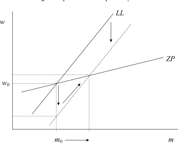
Equations (ZP) and (LL) determine the long-run values of the endogenous variables m and w. The equilibrium is shown in Figure 2, which plots these two equations in (m; w)-space. Note that (ZP) and (LL) are both positively sloped. We have drawn (ZP) as less steep than (LL), because otherwise scale economies would be so strong that the dynamic behavior of the model would be unstable under reasonable speci…cations. This amounts to assuming that is not too large.4
2.2
Short-run equilibrium
In short-run equilibrium we require labor markets to clear but takemas …xed. This means we are always on the (LL) schedule, with the wage rate determined by equation (LL) for a givenm.
4We note that in view of the positive slopes of both schedules, the model readily admits a multiplicity of long-run equilibria. Those equilibria whereZP crossesLLfrom below would be dynamically unstable under the dynamic speci…cation postulated below. So there would need to be at least three intersections for there to exist two stable long-run equilibria. We thank a referee for bringing the issue of multiplicity to our attention.
2.3
Dynamics
Given our assumptions so far, ifm were allowed to adjust instantaneously we would jump immediately to the long-run equilibrium given by the intersection of the (ZP) and (LL) schedules. In fact, forward-looking behavior on the part of investors in the modern sector provides an additional mechanism for immediate convergence to the long-run equilibrium. Suppose, for example, that we start at a level of m which falls short of m . On the transition to the long-run equilibrium, we know thatmandwwill both rise. Consider how these dynamics in‡uence the decision to enter. The rise in m implies that productivity will be higher in the future than it is today, and is a force that will induce delay in the decision to invest in the modern sector ceteris paribus. The rise inw, on the other hand, implies that investment will be more costly in the future than it is today, and is a factor that will precipitate investment. Given the relative slopes we have assumed, the second factor outweighs the …rst–i.e., wages increase faster than the rate at which productivity bene…ts come in–and investors would rather invest today than wait.
To provide the model with some non-trivial dynamics, we can simply assume that there is a limit to how much investment is feasible per unit of time. To be concrete, let the rate at whichm increases be restricted by the exogenous parameter . That is
: m(t)
Given the considerations discussed in the previous paragraph, there will be maximal adjustment inmwhenever net returns at timetare non-zero. Hence,
:
m(t) = if r(p;h;m(t)) > bw(t)
:
m(t) = if r(p;h;m(t)) < bw(t)
:
m(t) = 0 otherwise
2.4
Comparative dynamics
We are now ready to analyze the behavior of the economy. Starting from an initial equilibrium given by(m0; w0), consider an increase in the economy’s labor endowment. This shifts theLLschedule down since, at a givenm, labor-market equilibrium requires lower wages. Hence the impact e¤ect of larger L
is a lowerw. However, the lower wage induces more …rms to enter the modern sector and engage in cost discovery, which in turn pulls wages up. How high do wages eventually go? As Figure 2 shows, the new equilibrium is one where wages are higher than in the initial equilibrium. A larger labor endowment ends up boosting wages! What is key for this result is the presence of information spillovers in the modern sector. Once the modern sector expands, productivity rises, and zero pro…ts can be restored only if wages go up.
Increases inpandhoperate by shifting theZPschedule up. They both result in highermandweventually. An increase inb, the …xed cost of entry into the
modern sector, shifts both schedules down, and under the stability assumptions made previously yields lowerm and w. These results are less surprising, but have important policy implications. In particular, they imply that trade policies that raisep(import restrictions or export subsidies, depending on the context) would promote entrepreneurship and raise growth.
2.5
Discussion
Our framework is obviously related to models in the endogenous-growth tradi-tion that we cited earlier (see footnote 2), where there are externalities in the imitation and innovation process. Models of that kind also generate the result that entrepreneurial activity is too low in the laissez-faire equilibrium. What is di¤erent in our approach is that it identi…es a potentially empirically veri…able relationship between thetype of goods that an economy specializes in and its rate of economic growth. In our framework anything that pushes the economy to a higher max–to specialize in good(s) with higher productivity levels–sets forth a dynamic (if temporary) process of economic growth as emulators are drawn in to produce the newly discovered high-productivity good(s). In the empirical work below, we will try to document this particular link by develop-ing an empirical proxy for max and examining its relationship with growth.
3
Empirics
The model shows that productivity in the modern sector is driven by max, which depends onm, which in turn is driven by country size (L), human capital (h), and other parameters. In our empirical work, we shall proxy max with a measure calculated from export statistics which we callEXP Y. This measure aims to capture the productivity level associated with a country’s exports. Fo-cusing on exports is a sensible strategy since maxrefers to the most productive goods that a country produces and we can expect a country to export those goods in which it is the most productive. Consider for example a model of the world economy in which countries di¤er only in terms of their location in the product space depicted in Figure 1. In this model, comparative and absolute advantage would be aligned, and countries that export higher maxgoods would be richer precisely because they export those goods. Focusing on exports makes sense also for the practical reason that we have much more detailed data on exports across countries than we do on production.
In order to calculate EXP Y we rank commodities according to the income levels of the countries that export them. Commodities that are exported by rich countries (controlling for overall economic size) get ranked more highly than commodities that are exported by poorer countries. With these commodity-speci…c calculations, we then construct country-wide indices.
3.1
Construction of
EXP Y
First, we construct an index calledP RODY. This index is a weighted average of the per capita GDPs of countries exporting a given product, and thus represents the income level associated with that product. Let countries be indexed byj
and goods be indexed byl. Total exports of countryj equals
Xj =
X
l xjl
Let the per-capita GDP of country j be denoted Yj. Then the productivity
level associated with productk,P RODYk, equals P RODYk=
X
j
(xjk=Xj)
P
j(xjk=Xj) Yj
The numerator of the weight,xjk=Xj, is the value-share of the commodity in the
country’s overall export basket. The denominator of the weight,Pj(xjk=Xj),
aggregates the value-shares across all countries exporting the good. Hence the index represents a weighted average of per-capita GDPs, where the weights correspond to the revealed comparative advantage of each country in goodk.
The rationale for using revealed comparative advantage as a weight is to ensure that country size does not distort our ranking of goods. Consider an ex-ample involving Bangladesh and US garments, speci…cally, the 6-digit product category 620333, “men’s jackets and blazers, synthetic …ber, not knit.”In 1995, the US export value for this category was $28,800,000, exceeding Bangladesh’s export value of $19,400,000. However, this commodity constituted only 0.005 percent of total US exports, compared to 0.6 percent for Bangladesh. As de…ned above, theP RODY index allows us to weight Bangladesh’s income more heav-ily than the U.S. income in calculating the productivity level associated with garments, even though the U.S. exports a larger volume than Bangladesh.
The productivity level associated with countryi’s export basket,EXP Yi, is
in turn de…ned by
EXP Yi=
X
l xil Xi
P RODYl
This is a weighted average of theP RODY for that country, where the weights are simply the value shares of the products in the country’s total exports.5
3.2
Data and methods
Our trade data come from two sources. The …rst is the United Nations Com-modity Trade Statistics Database (COMTRADE) covering over 5000 products 5As we noted in the introduction, Michaely (1984) previously developed a similar index and called it "income level of exports." Michaely used a di¤erent weighting scheme in generating what we callP RODY, with each country’s weight corresponding to the market share in global exports of the relevant commodity. Compared to ours, therefore, Michaely’s approach over-weights large countries. Michaely’s calculations were undertaken for 3-digit SITC categories. More recently, Lall et al. (2005) have also developed a similar measure that they call the "sophistication level of exports."
at the Harmonized System 6-digit level for the years 1992 to 2003. The value of exports is measured in current US dollars. The number of countries that report the trade data vary considerably from year to year. However, we constructed theP RODY measure for a consistent sample of countries that reported trade data in each of the years 1999, 2000 and 2001. It is essential to use a consistent sample since non-reporting is likely to be correlated with income, and thus, con-structingP RODY for di¤erent countries during di¤erent years could introduce serious bias into the index. While trade data were actually available for 124 countries over 1999-2001, the real per capita GDP data from the World Devel-opment Indicators (WDI) database was only available for 113 of these countries. Thus, with the COMTRADE data, we calculateP RODY for a sample of 113 countries. We calculate P RODY using both PPP-adjusted GDP and GDP at market exchange rates. In what follows we shall present most of our results only with the PPP-adjusted measures ofP RODY; we have found no instance in which using one instead of the other makes a substantive di¤erence.
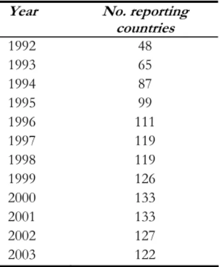
The average P RODY from 1999-2001 is then used to construct anEXP Y
measure for all countries reporting trade data during the period from 1992 to 2003. Since the number of countries reporting COMTRADE data varies from year to year, and the coverage is especially patchy for earlier years, the total number of countries for which we could calculateEXP Y ranges from a low of 48 in 1992 to a high of 133 in 2000. Table 1 shows the country coverage for each of the years between 1992 and 2003.
Some limitations of COMTRADE data are its relatively short time-span and limited coverage of countries earlier in the period. To check the robustness of our …ndings against these concerns, we have also constructed our measures with the World Trade Flows dataset which has recently been updated to extend coverage back to 1962 (Feenstra et al. 2005). Trade ‡ows are based on 4-digit standard international trade classi…cations (SITC rev. 2) comprising over 700 commodities. OurP RODY andEXP Y indices are calculated by combining the World Trade Flows data on export volumes with PPP-adjusted GDP from the Penn World Tables, yielding a sample of 97 countries for the period 1962-2000. We prefer to work with the indices based on more disaggregated data, and the basic patterns in the data are very much consistent between the two datasets. Hence we limit our discussion of descriptive statistics below to the COMTRADE data. We return to the 4-digit data when we turn to growth regressions.
3.3
Descriptive statistics
Some descriptive statistics on P RODY are shown in Table 2. The …rst row showsP RODY calculated using GDP at market exchange rates and the second row shows P RODY with PPP-adjusted GDP levels. As the table reveals, the income level associated with individual traded commodities varies greatly, from numbers in hundreds (of 2000 US dollars) to tens of thousands. This re‡ects the fact that specialization patterns are highly dependent on per-capital incomes.
The …ve commodities with the smallest and largest P RODY values are shown in Table 3. As we would expect, items with low P RODY tend to
be primary commodities. Consider for example product 10120, “live asses mules and hinnies.” The main reason this product has the lowest income level is that it constitutes a relatively important part of the exports of Niger, a country with one of the lowest per capita GDPs in our sample. Similarly, sisal, cloves, and vanilla beans have low P RODY values because they tend to be signi…cant exports for poor sub-Saharan African countries. On the other hand, product 7211060, ‡at rolled iron or non-alloy steel, has the highestP RODY
value because it holds a substantial share of Luxembourg’s exports, and this country has the highest per capita GDP in our sample.
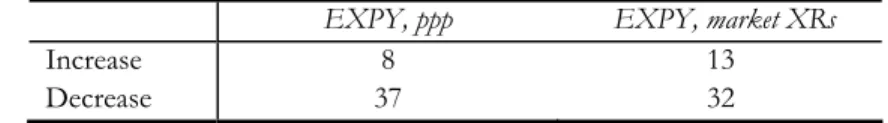
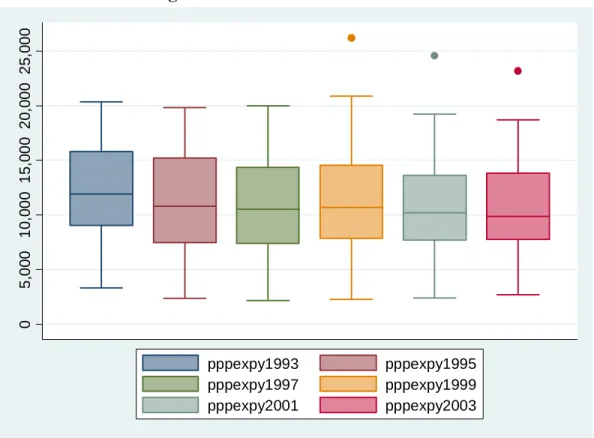
Table 4 and Figure 3 summarize some basic descriptive statistics forEXP Y. We note that the meanEXP Y for the sample of countries included exhibits a downward trend over time. MeanEXP Y has fallen from $12,994 in 1992 to $10,664 in 2003. Since the income levels associated with individual products are held constant over time (as explained above), this is due partly to the changing composition of the sample of countries (with more low-EXP Y countries being included over time) and partly to the reduction inEXP Y levels in many of the countries. Indeed, Table 5 shows that a majority of countries (among those that have EXP Y values throughout our sample period) have experienced a reduction inEXP Y over time. This downward trend may be speci…c to the recent period and dependent on levels of aggregation, since we do not see a similar trend since the 1960s when we use 4-digit trade data.
How does EXP Y vary across countries? Figure 4 shows a scatterplot of
EXP Y against per-capita GDP. Unsurprisingly, there is a very strong corre-lation between these two variables. The correcorre-lation coe¢ cient between the two is in the range 0.80-0.83 depending on the year. Rich (poor) countries export products that tend to be exported by other rich (poor) countries. Although in our framework this relationship has a di¤erent interpretation, it can also be explained with the Heckscher-Ohlin framework if rich country goods are more intensive in human capital or physical capital. The relationship betweenEXP Y
and per capita GDP exists partly by construction, since a commodity’sP RODY
is determined by the per capita GDPs of the countries that are important ex-porters of that commodity. However, the relationship is not just a mechanical one. Calculating country speci…cP RODYs by excluding own exports from the calculation of these measures does not change the results much. Note also that the variation in EXP Y across countries is much lower than the variation in per-capita GDPs. This is a direct consequence of the fact thatP RODY (and thereforeEXP Y) is a weighted average of national income levels.
Table 6 shows the countries with smallest and largestEXP Y values for 2001 (the year with the largest possible sample size). Note that French Polynesia (PYF) ranks in the top 5 among those with the largestEXP Y. This surpris-ing outcome arises in part because cultured pearl exports contribute heavily to a French Polynesia’s export basket and this product has a relatively large
P RODY value of $22,888. A few other cases where countries appear to have very largeEXP Y values relative to per capita GDP are Mozambique (MOZ), Swaziland (SWZ), Armenia (ARM), India (IND), and China (CHN). In a couple of these instances, the culprit is once again a speci…c commodity with a high
P RODY value: unwrought, alloyed aluminum for Mozambique and "mixed odoriferous substances in the food and drink industries" for Swaziland. But in the remaining cases (China, India, and Armenia), this is the result of a portfolio of a highP RODY exports, and not one or two speci…c items. At …rst sight, diamonds seem to play a large role in India and Armenia, but both countries retain their high EXP Ys even with diamonds removed from the calculation. And China has a very diversi…ed set of exports, with no single product category standing out in terms of high export shares. It is worth remembering at this juncture that China and India have both been experiencing very rapid economic growth (as has Armenia more recently) .
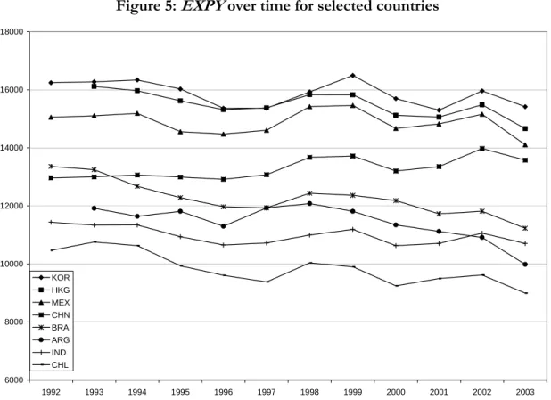
Figure 5 shows the time trend for EXP Y for China, India, and a sample of other Asian and Latin American countries. Among the Latin American countries included (Argentina, Brazil, Chile, and Mexico), only Mexico has a level ofEXP Y that is comparable to those in East Asia. This probably re‡ects the fact that the exports of the other three are heavily based on primary products and natural resources, which tend to have lowerEXP Ys. Chile has the lowest
EXP Y by far, and its EXP Y has been steadily drifting downwards. At the other end, South Korea and Hong Kong have the highestEXP Y s. Note how China has signi…cantly closed the gap with these countries over time. China’s
EXP Y has converged with that of Hong Kong, even though Hong Kong’s per capita GDP remains …ve times larger (in PPP-adjusted terms). And China’s
EXP Y now exceeds those of Brazil, Argentina, and Chile by a wide margin, even though China’s per-capita GDP is roughly half as large as those of the Latin American countries (see Rodrik [2006] and the related work of Schott [2006] for more detail on China). India’sEXP Y is not as spectacular as China’s, but that is in large part because our measure is based on commodity exports and does not capture the explosion in India’s software exports. Nonetheless, by 2003 India had a higher EXP Y than not only Chile, but also Argentina, a country that is roughly four times richer.6
Do all natural-resource exporting countries have low EXP Ys? Figure 6 shows a similar chart for …ve primary-product exporting countries: Canada, Norway, New Zealand, Australia, and Chile. The variation in EXP Y among these countries turns out to be quite large. Once again, Chile is at the bottom of the scale. But even among the remaining four advanced countries, the range is quite wide. Canada’sEXP Y is between 20-25 percent larger than Norway’s or Australia’s. Therefore, our measure seems to capture important di¤erences among primary product exporting countries as well.
3.4
Determinants of
EXP Y
What might be some of the fundamental determinants of the variation across countries in levels ofEXP Y? We have shown above thatEXP Y is highly cor-6We note that theEXP Yindex does not correct for di¤erences in quality within a product ctegory. even though we are working with highly disaggregated product categories, there is still wide variation in the unit values of goods produced by di¤erent countries. See Rodrik (2006) for the case of China.
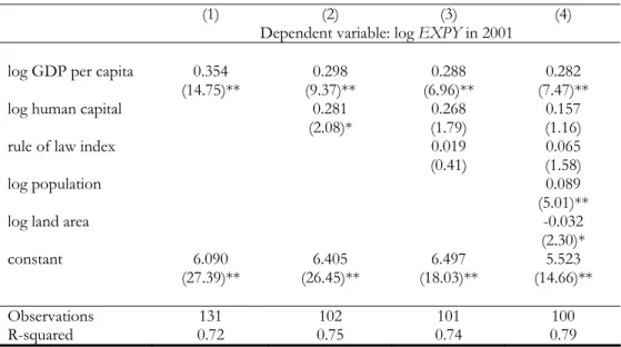
related with per-capita GDP. The model laid out in the early part of the paper suggests that specialization patterns will be determined both by fundamentals and by idiosyncratic elements. Among fundamentals, the model pointed to human capital and the size of the labor force as two key determinants. The …rst extends the range of "discoverable" goods, and the second promotes cost discovery through (initially) lower wages. We …nd support for both of these implications in the cross-national data. Human capital and country size (prox-ied by population) are both associated positively withEXP Y, even when we control for per capita GDP separately (Table 7). It may be di¢ cult to give the relationship with human capital a direct causal interpretation, since the causal e¤ect may go from EXP Y to human capital rather than vice versa. But it is easier to think of the relationship with country size in causal terms: it is hard to believe that there would be reverse causality from EXP Y to population size. Interestingly, institutional quality (proxied by the Rule of Law index of the World Bank, a commonly used measure of institutional quality) does not seem to be strongly associated withEXP Y once we control for per capita GDP (Table 7, column 3). This makes it less likely thatEXP Y is a proxy for broad institutional characteristics of a country.
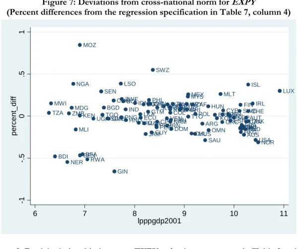
Even if we ascribe a causal role to per-capita income and human capital, there is a lot that remains unexplained in the determination ofEXP Y. Figure 7 shows a scatter plot of deviations from the cross-country norms established in column 4 of Table 7 against per capita GDP. There are big outliers in either direction, especially among low-income countries. Mozambique (+88 percent), Swaziland (+55 percent), and Senegal (+29 percent) haveEXP Y levels that are much higher than would be predicted on the basis of the right-hand side variables in Table 7, while Guinea 66 percent), Niger 55 percent), and Burundi (-57 percent) have much lower EXP Ys. If indeed such di¤erences matter to subsequent economic performance (and we claim that they do), it is important to understand where they arise from. Moreover, to the extent that EXP Y
levels exert an independent in‡uence on per capita income levels and human capital stocks, the "unexplained" component of the cross-national variation in
EXP Y is naturally much larger. Hausmann and Rodrik (2003) provide some anecdotal evidence which suggests that successful new industries often arise for idiosyncratic reasons. Fundamentals are only part of the story.
3.5
EXP Y
and growth
We …nally turn to the relationship betweenEXP Y and economic growth. We analyze this relationship in both cross-national and panel setings and using a wide variety of estimation techniques.
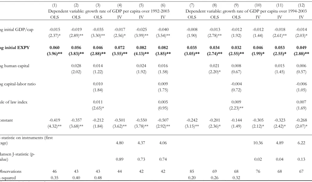
Table 8 shows a set of cross-national regressions in which growth is regressed on initial values ofEXP Y and other regressors. The maximum time span that we can use for these regressions based on COMTRADE data is a time horizon of 11 years (1992-2003). However, this leaves us with a sample of only some 40 odd countries. By focusing on a somewhat shorter time horizon–between 1994 and 2003–we can nearly double the sample of countries included in the
regres-sion. The table shows results with both samples. All regressions include initial per-capita GDP as a covariate. We also include human capital as a regressor, since it plays a role in our theoretical speci…cation. We add the (physical) capital-labor ratio and a rule of law index as well to account for neoclassical explanations for economic growth. Finally, we show both OLS and IV results. We appeal to the theory developed previously and the empirical results above in using country size (population and land area) as instruments in the IV speci-…cation. Country size is plausibly exogenous with respect toEXP Y levels and economic growth. But excludability from the second-stage regression can be viewed as more problematic. Many endogenous growth theories contain scale e¤ects–operating through channels other than what we have emphasized here– and would in principle call for country size to be introduced as an independent regressor in growth regressions. We take comfort and refuge in the fact that it has been very di¢ cult to …nd such scale e¤ects in growth empirics. Rose (2006) has recently undertaken a comprehensive empirical analysis looking for such scale e¤ects and reports decisively negative results.7 In light of such …nd-ings, our use of country size as an instrument seems plausible. We also note that we will use …xed-e¤ects and an alternative instrumentation strategy when we turn to panel estimation.
EXP Y enters with a large and positive coe¢ cient that is statistically signif-icant in all of these speci…cations. The estimated coe¢ cient varies from 0.032 to 0.082, with IV estimates being larger than OLS estimates.8 Taking the mid-point of this range, the results imply that a 10 percent increase inEXP Y boosts growth by half a percentage points, which is quite large. Figure 8 shows a repre-sentative scatter plot. Human capital, physical capital, and institutional quality do not enter in a robustly signi…cantly way, and their presence does not a¤ect much the signi…cance ofEXP Y. These results suggest that EXP Y exerts an indepedent force on economic growth and that it is not a proxy for the factor or institutional endowments of a country.
A shortcoming of these regressions is that the time horizon is short, and that they su¤er, as with all cross-national speci…cations, from possible omitted variables bias. While 6-digit disaggregation based on COMTRADE does not allow us to examine pre-1992 data, 4-digit calculations based on World Trade Flows allows us to construct a panel going back to 1962. Table 9 shows results from panel regressions. Data are grouped into 5- and 10-year intervals and four di¤erent estimators are used: pooled OLS, IV, OLS with …xed e¤ects (for countries and years), and GMM. (See notes at the bottom of the table for more 7Rose summarizes his results thus: "There is little evidence that countries with more people perform measurably better. Indeed, a good broad-brush characterization is that a country’s population has no signi…cant impact on its well-being" (2006, 15). The only exception that Rose notes is the well-known regularity that smaller countries have higher shares of trade in GDP.
8F-tests in IV speci…cations always indicate that instruments are jointly signi…cant in the …rst stage. Overidenti…cation tests using the J-statistic cannot reject excludability in columns (4)-(6). However, in columns (10)-(12) covering a shorter period, the null hypothesis of zero correlation of instruments with second-stage residuals is rejected in two of the three speci…cations.
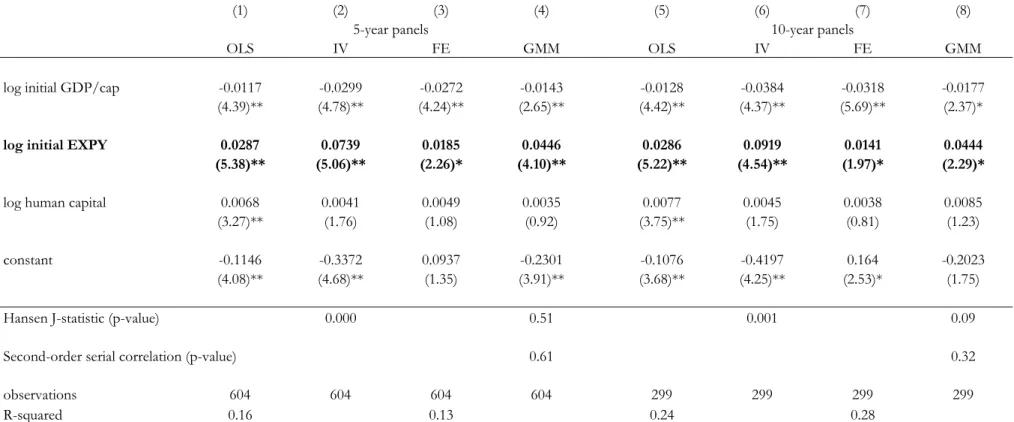
details.) The estimated coe¢ cient on EXP Y is signi…cant in all cases, with a magnitude that is comparable to that in the cross-section results reported above.9 The …xed e¤ects results are particularly telling, since these explicitly control for time-invariant country characteristics and identify the impact of
EXP Y o¤ the variation within countries. They are signi…cant in both the 5-and 10-year panels. These …xed e¤ects estimates suggest that a 10 percent increase inEXP Y raises growth by 0.14 to 0.19 percentage points. This is a smaller e¤ect than what we found in the cross-national speci…cations, but it is still noteworthy.
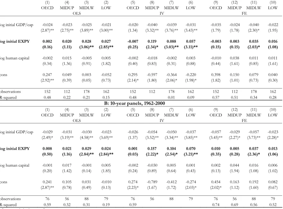
There is no reason a priori to expect thatEXP Y works the same way for all countries, and the panel regressions allow us to check for heterogeneity in its estimated impact on growth across di¤erent country subgroups. Table 10 shows various panel speci…cations estimated separately for four di¤erent coun-try groups distinguished by income levels: high-income OECD countries, upper middle-income countries (MIDUP), lower middle-income countries (MIDLW), and low income countries. We …nd thatEXP Y enters most strongly in coun-tries at intermediate income levels. The …xed-e¤ects point estimate for the MIDLW sub-sample suggests that a 10 percent increase inEXP Y boosts growth by 0.35-0.37 percentage points, double the estimate for the sample as a whole and close to the cross-section estimate. Interestingly,EXP Y never enters sig-ni…cantly in the OECD sub-sample. This is perhaps because rich countries have fairly stableEXP Y values: the standard deviation of EXP Y is half as large in the OECD sub-sample as it is in the rest of the sample. In …xed-e¤ects regressions, the results in the lowest-income sub-sample are very poor as well, possibly re‡ecting considerable measurement error (in trade statistics over time) for this sub-sample. So with respect to the within-variation,EXP Y does a much better job distinguishing performance among middle-income countries than among countries at either end of the income spectrum.
We have subjected these results to a large number of additional robustness tests, which we do not report for reasons of space. In particular, both the cross-national and panel results are robust to the inclusion of additional covariates such as distance from the equator, legal origin dummies and measures of …-nancial development (e.g., private credit as a share of GDP). Even with these controls, EXP Y remains statistically signi…cant and of similar magnitude in each of the twelve equations in Table 8, except in the last three. In the panel, the additional controls do not materially change the signi…cance or magnitude ofEXP Y in any of the 5-year results. All of the 10-year results are also pre-served, except in the case of GMM, where the coe¢ cient is no longer signi…cant although its magnitude remains the same.
9The variables used as instruments fail the overidenti…cation test in columns (2) and (6), most likely because they are very persistent and are akin to country …xed e¤ects in a panel. Re-assuringly, columns (4) and (8) show that the GMM setup where lagged levels and di¤erences are used as instruments passes both the overidenti…cation test and exhibits no second-order correlation.
3.6
Discussion
Our results show that countries that export goods associated with higher pro-ductivity levels grow more rapidly, even after we control for initial income per head, human capital levels, and time-invariant country characteristics. What is the economic mechanism that drives this growth? In the simple model we sketched out, growth is the result of transferring resources from lower-productivity activities to the higher-lower-productivity goods identi…ed by the entre-preneurial cost-discovery process. An important characteristic of these goods is that there is elastic demand for them in world markets, so that a country can export them in large quantities without signi…cant adverse terms-of-trade e¤ects. As an indication of this mechanism, we …nd, for example, that countries with initially high levels of EXP Y subsequently experience higher growth in exports (see Figure 9).10
Fostering an environment that promotes entrepreneurship and investment in new activities would appear therefore to be critical to economic convergence. From an allocative-e¢ ciency standpoint, the key is that such activities generate information spillovers for emulators (on which see Hausmann and Rodrik [2003] for more discussion and evidence). A full discussion of the policy implications of this is beyond the scope of the present paper (see Rodrik [2004]). But, generically, the requisite policy is to subsidize initial entrants in new activities (but not followers).
More broadly, our results suggest that the type of goods in which a country specializes has important implications for subsequent economic performance. Everything else being the same, an economy is better o¤ producing goods that richer countries export.11 Standard models of comparative advantage indicate that pushing specialization up the product scale in this fashion would be bad for an economy’s health: it would simply distort production and create e¢ ciency losses. The framework we developed in the paper, and the evidence that we o¤ered, suggest an alternative interpretation. A country’s fundamentals gen-erally allow it to produce more sophisticated goods than it currently produces. Countries can get stuck with lower-income goods because entrepreneurship in cost discovery entails important externalities. Countries that are able to over-come these externalities–through policies that entice entrepreneurs into new 1 0A complementary mechanism is that countries that start producing sophisticated products can grow more rapidly as they experience convergence to the quality frontier in those goods. Work by Hwang (forthcoming) has found strong evidence of unconditional convergence in product quality (measured by unit values) at the level of individual products.
1 1A question arises as to whether it is possible for all countries to do this in the general equilibrium of the world economy. In a world with homogeneous goods, it would be impossible for all countries to move "upscale" as some goods would not be produced at all and the gains from trade would disappear. But in a world with di¤erentiated goods, it is possible to envisage poor countries producing more of the "types" of goods that rich countries produce and trading these "varieties" against those that rich countries produce. Still, for poor countries there may be compensating terms-of-trade bene…ts from producing goods that are dissimilar to "rich-country" goods. Our analysis does not track these potential gains/losses since we are focusing on growth in output (not income, which is what the terms of trade a¤ect). We thank an anonymous referee for bringing these issues to our attention.
activities–can reap the bene…ts in terms of higher economic growth.
4
Concluding remarks
What we have shown in this paper is that there are economically meaningful di¤erences in the specialization patterns of otherwise similar countries. We have captured these di¤erences by developing an index that measures the "quality" of countries’export baskets. We provided evidence that shows that countries that latch on to a set of goods that are placed higher on this quality spectrum tend to perform better. The clear implication is that the gains from globalization depend on the ability of countries to appropriately position themselves along this spectrum.
5
References
Aghion, Philippe, Robin Burgess, Stephen Redding and Fabrizio Zilibotti, "En-try Liberalization and Inequality in Industrial Performance," Journal of the European Economic Association, 3 (2-3), 2005, 291-302.
Aghion, Philippe, and Peter Howitt, Endogenous Growth Theory, Cam-bridge, MA, MIT Press, 1998.
Banerjee, Abhijit, and Esther Du‡o, “Do Firms Want to Borrow More? Testing Credit Constraints Using a Directed Lending Program,” unpublished paper, MIT, 2004.
Banerjee, Abhijit, and Kaivan Munshi, “How E¢ ciently is Capital Allo-cated? Evidence from the Knitted Garment Industry in Tirupur,”Review of Economic Studies71(1), 2004, 19-42.
Barro, Robert, and Xavier Sala-i-Martin,Economic Growth, 2nd ed., Cam-bridge, MA, MIT Press, 2003.
Bernard, A. B., J. Eaton, J. B. Jensen, and S. Kortum, "Plants and Produc-tivity in International Trade,"American Economic Review 93, 2003, 1268-1290. Djankov, Simeon, Rafael La Porta, Florencio Lopez-de-Silanes and Andrei Shleifer, "The Regulation of Entry,"Quarterly Journal of Economics,117 (1), 2002, 1-37.
Evenson, Robert, and Larry E. Westphal, “Technological Change and Tech-nology Strategy,” ch. 37 in Jere Behrman and T.N. Srinivasan, eds.,Handbook of Development Economics, vol. 3A, Amsterdam, North-Holland, 1995, pp. 2209-2229.
Feenstra, Robert C., et al., "World Trade Flows, 1962-2000," NBER, Janu-ary 2005.
Fisman, Ray, "Estimating the Value of Political Connections," American Economic Review, 91 (4), 2001, 1095-1102.
Fujita, Masahisa, Paul Krugman, Anthony J. Venables, The Spatial Econ-omy: Cities, Regions, and International Trade, Cambridge, MA, MIT Press, 1999.
Grossman. Elhanan, and Gene Grossman, Innovation and Growth in the World Economy, Cambridge, MA, MIT Press, 1991.
Hausmann, R. and D. Rodrik, "Economic Development as Self Discovery,"
Journal of Development Economics, December 2003.
Hummels, David, and Peter J. Klenow, "The Variety and Quality of a Na-tion’s Exports,"American Economic Review, vol. 95, no. 3, June 2005, 704-723. Hwang, Jason, “Introduction of New Goods, Convergence, and Growth,” Department of Economics, Harvard University, 2006, forthcoming.
Lall, Sanjaya, "Skills, Competitiveness and Policy in Developing Countries," Queen Elizabeth House Working Paper QEHWPS46, University of Oxford, June 2000.
Lall, Sanjaya, John Weiss, and Jinkang Zhang, "The ’Sophistication’of Ex-ports: A New Measure of Product Characteristics," Queen Elisabeth House Working Paper Series 123, Oxford University, January 2005.
Matsuyama, Kiminori, "Agricultural Productivity, Comparative Advantage, and Economic Growth,"Journal of Economic Theory, December 1992, 317-334. McKenzie, David, and Christopher Woodru¤, “Do Entry Costs Provide an Empirical Basis for Poverty Traps? Evidence from Mexican Microenterprises,” unpublished paper, Stanford University, 2003.
Melitz, Marc J., and Gianmarco I.P. Ottaviano, "Market Size, Trade, and Productivity," Harvard University, October 10, 2005.
Michaely, Michael, Trade, Income Levels, and Dependence, North-Holland, Amsterdam, 1984.
Porter, Michael E.,The Competitive Advantage of Nations, New York: The Free Press. 1990.
Rodrik, Dani, "Industrial Policies for the Twenty-First Century," Harvard University, October 2004.
Rodrik, Dani, “What’s So Special About China’s Exports?”China & World Economy, vol. 14. no. 5, September-October, 2006, 1-19.
Rose, Andrew K., "Size Really Doesn’t Matter: In Search of A National Scale E¤ect," NBER Working Paper No. 12191, April 2006.
Sachs, J., and A.Warner, “Natural Resource Abundance and Economic Growth,” in G. Meier and J. Rauch (eds.),Leading Issues in Economic Development, New York: Oxford University Press, 1995.
Sala-i-Martin, Xavier, and Arvind Subramanian, "Addressing the Natural Resource Curse: An illustration from Nigeria," IMF Working Paper, July 2003. Schott, Peter, "Across-Product versus Within-Product Specialization in In-ternational Trade,"Quarterly Journal of Economics, 119(2), May 2004, 647-678. Schott, Peter, "The Relative Sophistication of Chinese Exports," NBER Working Paper 12173, April 2006.
Stokey, Nancy, "Learning-by-Doing and the Introduction of New Goods,"
Journal of Political Economy, 96, 1988, 701-717.
Svensson, Jakob, "Who Must Pay Bribes and How Much? Evidence from a Cross Section of Firms,"Quarterly Journal of Economics, 118 (1), 2003, 207-30. Young, Alwyn, "Learning by Doing and the Dynamic E¤ects of International Trade,"Quarterly Journal of Economics, 106, 1991, 369-405.
Table 1: Sample size of
EXPY
Year No. reporting
countries
1992 48 1993 65 1994 87 1995 99 1996 111 1997 119 1998 119 1999 126 2000 133 2001 133 2002 127 2003 122
Table 2: Descriptive statistics for
PRODY
(2000 US$)
Variable No. obs. Mean Std. Dev. Min Max
mean PRODY, 1999-2001,
at market exchange rates 5023 11,316 6,419 153 38,573
mean PRODY, 1999-2001,
PPP-adjusted 5023 14,172 6,110 748 46,860
Table 3: Largest and smallest
PRODY
values (2000 US$)
product product name mean PRODY, 1999-2001
smallest 140490 Vegetable products nes 748
530410 Sisal and Agave, raw 809
10120 Asses, mules and hinnies, live 823
90700 Cloves (whole fruit, cloves and stems) 870
90500 Vanilla beans 979
largest 721060 Flat rolled iron or non-alloy steel, coated with aluminium, width>600mm 46,860
730110 Sheet piling of iron or steel 46,703
721633 Sections, H, iron or non-alloy steel, nfw hot-roll/drawn/extruded > 80m 44,688
590290 Tyre cord fabric of viscose rayon 42,846
Table 4: Descriptive statistics for
EXPY
(2000 US$)
Year Obs. Mean Std. Dev. Min Max
1992 48 12,994 4,021 5,344 20,757
1993 65 12,407 4,179 3,330 20,361
1994 87 11,965 4,222 2,876 20,385
1995 99 11,138 4,513 2,356 19,823
1996 111 10,950 4,320 2,742 20,413
1997 119 10,861 4,340 2,178 19,981
1998 119 11,113 4,621 2,274 20,356
1999 126 11,203 4,778 2,261 26,218
2000 133 10,714 4,375 1,996 25,248
2001 133 10,618 4,281 2,398 24,552
2002 127 10,927 4,326 2,849 24,579
2003 122 10,664 3,889 2,684 23,189
Table 5: Number of countries that show an increase/decrease in
EXPY
, 1992-2003
EXPY, ppp EXPY, market XRs
Increase 8 13
Decrease 37 32
Table 6: Countries with smallest and largest
EXPY
s
Reporter EXPY
Smallest Niger 2,398
Ethiopia 2,715
Burundi 2,726
Benin 3,027
Guinea 3,058
Largest Luxembourg 24,552
Ireland 19,232
Switzerland 19,170
Iceland 18,705
Table 7: Correlates of
EXPY
(1) (2) (3) (4)
Dependent variable: log EXPY in 2001
log GDP per capita 0.354 0.298 0.288 0.282
(14.75)** (9.37)** (6.96)** (7.47)**
log human capital 0.281 0.268 0.157
(2.08)* (1.79) (1.16)
rule of law index 0.019 0.065
(0.41) (1.58)
log population 0.089
(5.01)**
log land area -0.032
(2.30)*
constant 6.090 6.405 6.497 5.523
(27.39)** (26.45)** (18.03)** (14.66)**
Observations 131 102 101 100
R-squared 0.72 0.75 0.74 0.79
Robust t-statistics in parentheses
Table 8: Cross-national growth regressions
(1) (2) (3) (4) (5) (6) (7) (8) (9) (10) (11) (12)
Dependent variable: growth rate of GDP per capita over 1992-2003 Dependent variable: growth rate of GDP per capita over 1994-2003
OLS OLS OLS IV IV IV OLS OLS OLS IV IV IV
log initial GDP/cap -0.015 -0.019 -0.035 -0.017 -0.025 -0.040 -0.008 -0.013 -0.012 -0.012 -0.018 -0.014 (2.37)* (2.89)** (3.30)** (2.56)* (3.99)** (3.54)** (1.90) (2.78)** (1.92) (1.44) (2.61)** (2.03)*
log initial EXPY 0.060 0.056 0.046 0.072 0.082 0.082 0.035 0.034 0.032 0.046 0.053 0.049
(3.96)** (3.83)** (2.88)** (3.55)** (4.13)** (3.85)** (3.05)** (2.74)** (2.55)** (1.99)* (2.55)* (2.88)**
log human capital 0.028 0.014 0.024 0.016 0.021 0.008 0.015 0.006
(2.02) (1.22) (1.92) (1.58) (2.20)* (0.67) (1.45) (0.57)
log capital-labor ratio 0.010 0.009 -0.004 -0.006
(1.84) (1.75) (0.72) (1.05)
rule of law index 0.011 0.005 0.009 0.007
(2.65)* (0.95) (2.23)** (1.69)
constant -0.419 -0.357 -0.212 -0.501 -0.550 -0.507 -0.242 -0.201 -0.144 -0.305 -0.323 -0.268 (4.32)** (3.68)** (1.84) (3.62)** (3.78)** (2.92)** (3.15)** (2.36)* (1.49) (2.12)* (2.42)* (2.07)*
F-statistic on instruments (first
stage) 4.80 4.37 4.06 10.36 4.89 6.22
Hansen J-statistic
(p-value) 0.89 0.73 0.74 0.02 0.04 0.13
Observations 46 43 43 44 42 42 85 69 68 76 68 67
R-squared 0.35 0.40 0.48 0.20 0.26 0.32
Robust t-statistics in parentheses
Instruments for IV regressions: log population, log land area. * significant at 5% level; ** significant at 1% level
Table 9: Panel growth regressions, 1962-2000
(1) (2) (3) (4) (5) (6) (7) (8)
5-year panels 10-year panels
OLS IV FE GMM OLS IV FE GMM
log initial GDP/cap -0.0117 -0.0299 -0.0272 -0.0143 -0.0128 -0.0384 -0.0318 -0.0177 (4.39)** (4.78)** (4.24)** (2.65)** (4.42)** (4.37)** (5.69)** (2.37)*
log initial EXPY 0.0287 0.0739 0.0185 0.0446 0.0286 0.0919 0.0141 0.0444
(5.38)** (5.06)** (2.26)* (4.10)** (5.22)** (4.54)** (1.97)* (2.29)*
log human capital 0.0068 0.0041 0.0049 0.0035 0.0077 0.0045 0.0038 0.0085
(3.27)** (1.76) (1.08) (0.92) (3.75)** (1.75) (0.81) (1.23)
constant -0.1146 -0.3372 0.0937 -0.2301 -0.1076 -0.4197 0.164 -0.2023
(4.08)** (4.68)** (1.35) (3.91)** (3.68)** (4.25)** (2.53)* (1.75)
Hansen J-statistic (p-value) 0.000 0.51 0.001 0.09
Second-order serial correlation (p-value) 0.61 0.32
observations 604 604 604 604 299 299 299 299
R-squared 0.16 0.13 0.24 0.28
Robust t-statistics in parentheses
All equations include period dummies. IV regressions use log population and log area as instruments. Fixed effects (FE) include dummies for countries. GMM is the Blundell-Bond System-GMM estimator using lagged growth rates and levels as instruments. The GMM estimation also uses log population and log area as additional instruments.
Table 10: Panel growth regressions by income sub-groups
A: 5-year panels, 1962-2000
(1) (4) (3) (2) (5) (8) (7) (6) (9) (12) (11) (10)
OECD MIDUP MIDLW LOW OECD MIDUP MIDLW LOW OECD MIDUP MIDLW LOW
OLS IV FE
log initial GDP/cap -0.024 -0.023 -0.025 -0.021 -0.020 -0.040 -0.039 -0.031 -0.035 -0.024 -0.040 -0.022 (2.87)** (2.75)** (3.89)** (3.00)** (1.34) (3.32)** (3.76)** (3.43)** (1.79) (1.78) (2.30)* (1.95)
log initial EXPY 0.002 0.020 0.028 0.027 -0.007 0.119 0.088 0.057 -0.003 0.003 0.035 0.016
(0.16) (1.11) (3.06)** (2.85)** (0.25) (2.34)* (3.03)** (3.11)** (0.15) (0.15) (2.03)* (1.08)
log human capital -0.002 0.015 -0.005 0.005 -0.002 -0.018 -0.002 0.003 -0.010 0.038 0.011 0.011 (0.34) (1.36) (0.91) (1.82) (0.40) (0.83) (0.31) (0.88) (0.44) (1.61) (0.85) (1.61) cons 0.247 0.049 0.003 -0.052 0.295 -0.597 -0.364 -0.220 0.398 0.150 0.079 0.040 (2.92)** (0.39) (0.05) (0.73) (2.14)* (1.80) (2.06)* (1.98)* (1.82) (1.01) (0.73) (0.30)
observations 152 112 178 162 152 112 178 162 152 112 178 162
R-squared 0.48 0.22 0.21 0.15 0.48 0.01 0.09 0.57 0.51 0.34 0.28
B: 10-year panels, 1962-2000
(1) (4) (3) (2) (5) (8) (7) (6) (9) (12) (11) (10)
OECD MIDUP MIDLW LOW OECD MIDUP MIDLW LOW OECD MIDUP MIDLW LOW
OLS IV FE
log initial GDP/cap -0.029 -0.031 -0.030 -0.023 -0.026 -0.054 -0.050 -0.037 -0.057 -0.029 -0.057 -0.023 (2.49)* (3.19)** (4.58)** (3.69)** (1.37) (3.52)** (3.34)** (3.85)** (3.45)** (2.27)* (3.73)** (2.28)*
log initial EXPY 0.008 0.021 0.029 0.024 0.001 0.157 0.104 0.070 0.010 0.005 0.037 0.013
(0.50) (1.16) (2.84)** (2.84)** (0.03) (2.22)* (2.54)* (3.21)** (0.35) (0.28) (2.36)* (1.06)
log human capital -0.001 0.017 -0.001 0.005 -0.002 -0.030 0.005 0.001 0.002 0.044 0.016 0.006 (0.20) (1.42) (0.14) (1.85) (0.24) (0.89) (0.64) (0.43) (0.13) (1.94) (1.08) (1.02) cons 0.241 0.105 0.031 -0.010 0.274 -0.789 -0.412 -0.274 0.454 0.163 0.192 0.082 (2.87)** (0.78) (0.49) (0.13) (2.23)* (1.67) (1.72) (2.03)* (2.02)* (1.12) (1.60) (0.67)
observations 76 56 88 79 76 56 88 79 76 56 88 79
R-squared 0.59 0.32 0.31 0.19 0.59 0.74 0.69 0.56 0.52
Figure 1: The production space
Figure 2: Equilibrium and comparative dynamics
m
w
LL
ZP
m
0
w
0
Figure 3: How
EXPY
varies over time
0 5, 00 0 10 ,0 00 15 ,0 0 0 20 ,0 00 25 ,0 00 pppexpy1993 pppexpy1995 pppexpy1997 pppexpy1999 pppexpy2001 pppexpy2003Figure 4:
Relationship between per-capita GDP and
EXPY
, 2003
LUX IRL
CHE ISL FINJPNDEU SWEGBR USAAUTDNK SGPFRA
NLDCAN BEL ISR CZE
HUNKORSVN HKGITA ESP MEXMYS SVKPRTNZL
EST POL CHN ZAF THA AUS GRC BLZ NOR BRB HRV PHL TUR CRIBRAURYRUSLVALTU
BLR ARG ROM KNA BGR IND EGY WSM TTO IDN
COLMKDGRD LBN JOR CHL DZA SLV OMN MUS AZELKAVEN KAZIRN
PAN NGA MDABGD MARGTM
SEN GAB GEO BOL LCA BHR PER NAM ALB ECU CMR VCT PRY DMA NIC HND PNG TGO GUY UGA SDN MNG MDG KEN MWI CAF TZA RWA ETH NER FJI NPL ARM SYR CIV PAK KGZ BIH 8 8. 5 9 9. 5 10 lo g EXPY (2 0 0 3 )
6 7 8 9 10 11
Figure 5:
EXPY
over time for selected countries
6000 8000 10000 12000 14000 16000 18000
1992 1993 1994 1995 1996 1997 1998 1999 2000 2001 2002 2003 KOR
HKG MEX CHN BRA ARG IND CHL
Figure 6:
EXPY
over time for natural-resource exporting countries
8000 10000 12000 14000 16000 18000
CAN NZL AUS CHL NOR
Figure 7: Deviations from cross-national norm for
EXPY
(Percent differences from the regression specification in Table 7, column 4)
LUX IRL CHE ISL FIN JPN SWE AUT GBR USA DNK SGP MLT FRA NLD CAN BEL ISR HUN ITA KOR HKG ESP MEX NZL MYS PRT POL CHN ZAF CYP THA SWZ AUS GRC MOZ NOR BRB PHL RUS BRA URY TUR CRI ARG ROM IND EGY TTO IDN COL BWA JOR CHL LSO DZA SLV OMN MUS VEN LKA IRN SAU PAN DOM NGA MAR BGD GTM SEN GAB ZWEBOL PERNAM ECU CMR CPV PRY NIC HND JAM PNG TGO GUY UGA SDN MDG KEN GMB MWI ZMB TZA MLI BFA RWA GIN BEN BDI NER -1 -. 5 0 .5 1 pe rc en t_ di ff
6 7 8 9 10 11
lpppgdp2001
Figure 8: Partial relationship between
EXPY
and subsequent growth (Table 8, col. 5)
BDI TGO UGA MDGCAF MWI HND DMA PRY ECUBOL BGD NIC GTM LCA MAR COG VCT HTI SLV GAB VUT COL PER CRI GRD LKA NPL VEN MUS IDN BLZ TTO SAU DZAEGY JOR OMN CHL MDA KNAIND TUR MKD ROM ARG MLT LTU GRC BRA HRV CHN URY THA MYS POL LVA PRT SVK AUS HUN NOR MEX CZE NZL SVN HKG ESP KOR ITA NLD SGP FRA CANGBRUSA
AUTDNKSWE DEU FIN JPN IRL ISL CHE .2 5 .3 .3 5 .4 C o m p o n en t pl us r e s idu al
8 8.5 9 9.5 10
Figure 9: Relationship between EXPY and subsequent export growth
Note: This chart shows growth in exports over 1992-2003 as a function of the 1992 level of
EXPY (controlling for initial income).
MDG
PRY
BGD
JAM ECU
BOL LCA LKA COL
HTI
PER
KEN IDN
BLZCHL SAUOMN
TUR TTO
IND GRC
ROM
THA CYP
CHN
HRVPRT
MYS BRA
HUN
AUS MEX
ESP
KOR
NZLSGP NLD CAN
USA DNKSWEDEU
IRL
FIN ISL
CHE