Vol 4, No 11 (2013)

Available online through

ISSN 2229 – 5046

MATHEMATICAL MODEL

FOR OLIGOSACCHARIDE HYDROLYSIS: HOMOTOPY ANALYSIS METHOD

Anandan Anitha

1

_{, Shanmugarajan Anitha}

2

_{, Princy Patturani}

2

_{, Lakshmanan Rajendran}

2,*

1_{Inspector of Anglo-Indian Schools, Chennai-600006, Tamilnadu, India.}

2_{Department of Mathematics, The Madura college, Madurai-625011, Tamilnadu, India.}

(Received on: 17-09-13; Revised & Accepted on: 12-11-13)

ABSTRACT

A

mathematical model for oligosaccharide hydrolysis is discussed. This model is based on system of differential equations contains a non-linear term related to kinetics of the enzymatic reactions. Homotopy analysis method (HAM) is employed to solve the system of reaction equations for the steady-state condition. Simple and approximate analytical expressions for concentrations of isomaltohexaose (C6), isomaltotetraose (C4), isomaltotriose (C3) and isomaltose (C2) are derived for all values of kinetic constants, (Km and Vmax) and the selectivity coefficient (

α

). Furthermore, in this work the numerical solution of the problem is also reported using Scilab/Matlab program. The analytical results have been extended numerically and are found to be in good agreement in each other.

Keywords: Mathematical Modelling; Suspended enzyme; Kinetic parameters; Hydrolysis of oligosaccharide; Homotopy analysis method.

1. INTRODUCTION

Sugar industry has faced severe competition from new sweeteners so-called oligosaccharides. Various oligosaccharides such as isomalto- oligosaccharides, soybean- oligosaccharides and fructooligosaccharides are known to be sweeteners which are beneficial to human and animal health [1, 2]. Fructooligosaccharides represent one of the major classes of bifidogenic oligosaccharides in terms of their production volume. The oligosaccharide introduced so far, fructooligosaccharides constitute one of the most popular functional food components in some European countries. A chromatographic separation technique and a mixed enzyme system are the two methods for increasing the content of the oligosaccharide [3, 4]. Galacto-oligosaccharides (GOS) are non-digestible food ingredients that beneficially affect the host by selectively stimulating the proliferation of bifidobacteria, which is considered to be beneficial to human health. But, if this acceptor is a water molecule galactose is released through a hydrolysis reaction [5].

The vast majority of chemical transformations inside cells are carried out by proteins called enzyme. Enzyme is often used in a immobilized form in industry for the purpose of repeated or continuous uses. Enzyme –based biochemical are attractive for the determination of agricultural resources. Recently, it has been reported that oligosaccarides having physiological activity can be obtained by the enzymatical hydrolysis of oligosaccardie contained in agricultural waste [6]. Several researchers have attempted to construct the mathematical models that describe this consecutive depolymerization kinetics [7-12]. Fujii et al. [8, 9] have proposed a lumped model in which all oligomers and polymers other than a monomer were considered together as one substrate. In their model the differential equations following Michaelis-Menten kinetics were formulated for each substrate species with the various polymerization degrees. Dean and Rollings [7] have extended the mathematical model proposed by Suga et al. [11].

Shibasaki-Kitakawa et al. [13] described the experimental result of the hydrolysis kinetics of oligosaccharide using suspended and immobilized enzymes. To our knowledge, no general analytical expressions that describe the concentrations of isomaltohexaose (C6), isomaltotetraose (C4), isomaltotriose (C3) and isomaltose (C2) in suspended

enzyme for various values of the range of system parameters have been reported. However, in general, analytical solutions of non-linear differential equations are more important and very useful than purely numerical solutions, as they are amenable to various kinds of data manipulation and analysis. For this reason, the analytical expressions corresponding to the concentrations of isomaltohexaose, isomaltotetraose, isomaltotriose and isomaltose in suspended enzyme are derived using Homotopy analysis method [14-16].

Corresponding author: Lakshmanan Rajendran2,*

2. MATHEMATICAL FORMULATION OF THE PROBLEM

Using Michaelis-Menten kinetics and the selectivity coefficients, the rates of change in the concentration of the respective saccharides and enzyme-substrate complex are given as follows [13]:

6

2 6 1 6

3

k

C

_E

C

k

C

_ES

dt

dC

+

−

=

(1)

4

6 1 4 2

3

4

₍

₁

₎

ES E

ES

k

C

C

k

C

C

k

dt

dC

₌

₋

_α

₋

₊

(2)

6

3 3

2

k

C

ES

dt

dC

₌

_α

(3)

4

6 3

3

2

₍

₁

₎

₂

ES ES

k

C

C

k

dt

dC

₌

₋

_α

₊

(4)

0

)

(

3

6 6

3 2 6

1

−

+

=

=

_{E ES}

ES

C

k

k

C

C

k

dt

dC

(5)

0

)

(

4 4

3 2 4

1

−

+

=

=

_{E ES}

ES

C

k

k

C

C

k

dt

dC

(6)

The total concentration of enzyme in the system is

4 6

)

0

(

_{E ES ES}

E

C

C

C

C

=

+

+

(7) where

C

_i and

i

ES

C

are the concentration of the saccharides and the enzyme-substrate complex, in the solution

respectively. The subscript

i

is a counter corresponding to the polymerization degree of the saccharides and

k

₁,

k

₂

and

k

₃ are the rate constants. Eqs. (1)-(4) can be written as follows:

4 6

6 max 6

3

3

C

C

K

C

V

dt

dC

m

+

+

−

=

(8)

4 6

4 6 max

4

3

]

)

1

(

3

[

C

C

K

C

C

V

dt

dC

m

+

+

−

−

=

α

(9)

4 6

6 max 3

3

6

C

C

K

C

V

dt

dC

m

+

+

=

α

(10)

4 6

4 6 max

2

3

]

2

)

1

(

3

[

C

C

K

C

C

V

dt

dC

m

+

+

+

−

=

α

(11)

where the constants

1 3 2

k

k

k

K

m

+

=

and

V

_max

=

k

₃

C

_E

(

0

)

. The boundary conditions are

6

and

i

0 (

2, 3, 4)

C

=

a

C

=

i

=

at t = 0 (12)

3. ANALYTICAL EXPRESSION OF CONCENTRATION OF THE SACCHARIDES USING HOMOTOPY ANALYSIS METHOD

The Homotopy analysis method (HAM) is a powerful analytical method to solve nonlinear problems [14-16] and this method provides a convenient way to guarantee the convergence of approximation series. The Homotopy analysis method has the following advantages: It is valid even if a given nonlinear problem does not contain any small/large parameters at all; It can be employed to efficiently approximate a nonlinear problem by choosing different sets of base functions. Furthermore, the obtained result is of high accuracy. Solving the Eqs. (8) - (11) using Homotopy analysis method (see Appendix A), we can obtain the following concentrations:

















−

−

−

+

+

+

=

− −

− −

m m

m

m K

t V K

t V K

t V

m K

t V

e

e

e

K

ha

ae

t

C

max max

max

max ₂ 6 4 3

3

6

(

1

)

3

(

1

)

2

(

2

)

2

3

)

























−

−

−

−

+

+

















−

+

−

−

















−

−

=

− − − − − − − m m m m m m m K t V K t V K t V K t V K t V m K t V K t V

e

e

e

e

e

K

ha

e

e

a

t

C

max max max max max max max

)

2

11

(

4

)

2

(

6

)

5

4

(

2

)

1

(

3

4

)

1

(

3

2

)

1

(

3

)

(

3 4 2 6 2 3 4

α

α

α

α

α

α

(14)

















−

−

−

+

+

−

















−

=

− − − − m m m m K t V K t V K t V m K t V

e

e

e

K

ha

e

a

t

C

max max max

max ₂ 6 4 3

3

(

1

)

3

(

1

)

2

(

2

)

3

1

2

)

(

α

α

α

α

α

(15)





















+

−

+

+

+

−

+

−

−

−

















−

−

=

_{− −} − − − m m m m m K t V K t V K t V K t V m K t V

e

e

e

e

K

ha

e

a

t

C

max max max max max

)

2

1

(

16

)

1

(

6

53

)

2

(

4

)

11

2

(

4

)

1

(

3

1

)

1

(

3

)

(

2 3 4 2 2

α

α

α

α

α

α

α

(16)

The Eqs. (13) – (16) satisfy the boundary conditions Eq. (1). This equation represents the new analytical expression of concentration C6(t),C4(t),C3(t) and C2(t) for all possible values of the parameters

K

m,

V

max and

α

. Using Eq. (8) and Eq. (9) and the boundary condition Eq. (12), the following relation is obtained.

α

α

C

(

t

)

C

(

t

)

2

a

2

₆

+

₃

=

(17)

Our analytical results (Eq. (13) and Eq. (15)) also satisfies the above result.

4. NUMERICAL SIMULATION

The non-linear reaction equations (8) - (11) for the given boundary conditions are also solved numerically. The function pdex45 in Scilab/Matlab numerical software (Appendix B) is used to solve the initial-boundary value problems for parabolic-elliptic partial differential equations numerically. Its numerical solution is compared with the analytical results obtained using HAM method.

5. RESULTS AND DISCUSSION

Eqs. (8)-(11) is the new simple approximate analytical expression of concentrations of isomaltohexaose (C6),

isomaltotetraose (C4), isomaltotriose (C3) andisomaltose (C2) calculated using Homotopy analysis method. Figures

1((a) - (f)) represent the concentrations versus the time t for different values of parameters a,

α

,Vmax and K_m. In all of

figures, the isomaltohexaose simply decreases with the reaction time, while the isomaltotetraose, isomaltotriose and isomaltose concentrations increase, respectively. Finally, isomaltotetraose is also converted into isomaltose, and only isomaltotriose and isomaltose exist in the system. When the initial concentration of isomaltohexaose (C6(0)=a)

decreases from initial value to zero, there is a slight difference in the tendencies for the consumption of isomaltohexaose.

From these figures it is inferred that the concentration of isomaltohexaose (C6) is always a decreasing function from

the initial value (C6(0)=a). The concentration profile of isomaltose (C2) increases as time increases. The concentration

profile of isomaltose (C2) reaches the steady state value when

t

≥

150

min

. The concentration of isomaltotetraose

(C4) increases initially and attains its maximum value and then decreases. The concentration profiles of isomaltotriose

(C3) increase as time increases. The concentration profile of isomaltotriose (C3) reaches the steady state value when

min

100

≥

t

.

6. CONCLUSION

A non-linear time-dependent differential equation for the hydrolysis of oligosaccharide has been solved using the HAM. The primary result of this work is an approximate calculation of the concentration profiles of the isomaltohexaose (C₆), isomaltotetraose (C4), isomaltotriose (C3) and isomaltose (C2) for all values of the

ACKNOWLEDGEMENT

This work was supported by the Council of Scientific and Industrial Research (CSIR) No. 01(2442)/10/EMR-II, Government of India. The authors also thank the secretary, The Madura College Board, and the principal, The Madura College, Madurai, Tamil Nadu, India, for their support and encouragement.

Appendix - A

For convenience, we can take

u

=

C

₆

,

v

=

C

₄

,

w

=

C

₃

and

z

=

C

₂. In this Appendix, we indicate how Eqs. (8) – (11) are derived using Homotopy Analysis Method.









₊

₊

₊

=









₊

−

V

u

dt

du

v

u

K

ph

u

V

dt

du

K

p

)

_m

3

_max

(

_m

3

)

3

_max

1

(

(A.1)









₊

₊

₋

₋

₋

=









₋

₋

₋

−

)

(

3

(

1

)

)

(

3

)

(

3

(

1

)

)

1

(

_max

V

_max

u

v

dt

dv

v

u

K

ph

v

u

V

dt

dv

K

p

_m

α

_m

α

(A.2)









₊

₊

₋

=









₋

−

V

u

dt

dw

v

u

K

ph

u

V

dt

dw

K

p

)

_m

6

_max

α

(

_m

3

)

6

_max

α

1

(

(A.3)









₊

₊

₋

₋

₊

=









₋

₋

₊

−

)

(

3

(

1

)

2

)

(

3

)

(

3

(

1

)

2

)

1

(

max

V

max

u

v

dt

dz

v

u

K

ph

v

u

V

dt

dz

K

p

m

α

m

α

(A.4)

The approximate solutions of Eqs. (A.1) - (A.4) are as follows

...

2 2 1

0

+

+

+

=

u

u

p

u

p

u

(A.5)

...

2 2 1

0

+

+

+

=

v

v

p

v

p

v

(A.6)

...

2 2 1

0

+

+

+

=

w

w

p

w

p

w

(A.7)

...

2 2 1

0

+

+

+

=

z

z

p

z

p

z

(A.8)

Substituting Eq. (A.5) in Eq. (A.1), Eq. (A.6) in Eq. (A.2), Eq. (A.7) in Eq. (A.3) and Eq. (A.8) in Eq. (A4) equating the like powers of p, we get

0

3

:

max 0

0

0

+

=

u

V

dt

du

K

p

m _(A.9)

1 1 0

max 1 0 0

:

_m

du

3

(3

)

du

0

p

K

V

u

h u

v

dt

+

−

+

dt

=

(A.10)

and

0

)

1

(

3

:

max 0 max 0

0

0

−

−

+

=

v

V

u

V

dt

dv

K

p

m

α

_(A.11)

1 1 0

max 1 max 1 0 0

:

m

3

(1

)

(3

)

0

dv

dv

p

K

V

u

V

v

h u

v

dt

−

−

α

+

−

+

dt

=

(A.12)

and

0

6

:

max 0

0

0

−

=

u

V

dt

dw

K

p

m

α

_(A.13)

1 1 0

max 1 0 0

:

_m

dw

6

(3

)

dw

0

p

K

V

u

h u

v

dt

−

α

−

+

dt

=

(A.14)

and

0

2

)

1

(

3

:

0 _{max 0 max 0}

0

−

−

−

=

v

V

u

V

dt

dz

K

p

_m

α

_(A.15)

1 1 0

max 1 max 1 0 0

:

_m

dz

3

(1

)

2

(3

)

dz

0

p

K

V

u

V

v

h u

v

dt

−

−

α

−

−

+

dt

=

(A.16)

The initial conditions are as follows

0

and

0

,

0

,

_{0 0 0}

0

=

a

v

=

w

=

z

=

u

(A.17)

0

and

0

,

0

,

0

=

=

=

=

_{i i i}

i

v

w

z

From Eq. (A.9), Eq. (A.11), Eq. (A.13) and Eq. (A.15) and from the boundary conditions (A.17), we get m K t V

ae

t

u

max 3

0

(

)

−

=

(A.19)

















+

−

−

=

− − m m K t V K t V

e

e

a

t

v

max max 3 0

2

)

1

(

3

)

(

α

(A.20)

















−

=

− m K t V

e

a

t

w

max

1

2

)

(

0

α

(A.21)

















+

−

−

=

−

1

)

1

(

3

)

(

max 0 m K t V

e

a

t

z

α

(A.22)

Substituting the values of

u

₀

,

v

₀

,

w

₀

and

z

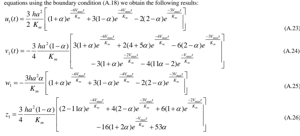
₀in Eq. (A10), Eq. (A12), Eq. (A14) and Eq. (A16) and solving the

equations using the boundary condition (A.18) we obtain the following results:

max max max

6 4 3

2

1

3

( )

(1

)

3(1

)

2( 2

)

2

m m m

V t V t V t

K K K

m

ha

u t

e

e

e

K

α

α

α

− − −





=



+

+

−

−

−











(A.23)





















−

−

+

−

−

−

+

+

+

−

−

=

_{− −} − − − m m m m m K t V K t V K t V K t V K t V m

e

e

e

e

e

K

ha

t

v

max max max max max

)

2

11

(

4

)

1

(

3

)

2

(

6

)

5

4

(

2

)

1

(

3

)

1

(

4

3

)

(

2 3 4 6 2 1

α

α

α

α

α

α

(A.24)

















−

−

−

+

+

−

=

− − − m m m K t V K t V K t V m

e

e

e

K

ha

w

max max

max 4 3

6 2

1

(

1

)

3

(

1

)

2

(

2

)

3

α

_α

_α

_α

(A.25)





















+

+

−

+

+

−

+

−

−

=

₋ − − −

α

α

α

α

α

α

53

)

2

1

(

16

)

1

(

6

)

2

(

4

)

11

2

(

)

1

(

4

3

max max max

max 3 2

4 2 1 m m m m K t V K t V K t V K t V m

e

e

e

e

K

ha

z

_(A.26)

When p=1, the approximate solution Eqs. (A.5)-(A.8) becomes

1 0 1 0 1 0 1 0

)

(

)

(

)

(

)

(

z

z

t

z

w

w

t

w

v

v

t

v

u

u

t

u

+

≈

+

≈

+

≈

+

≈

(A.27)

Adding Eq. (A.19) and Eq. (A.23), we get Eq. (12) in the text. Similarly we get Eqs. (13) – (15) in the text.

Appendix – B

Scilab/Matlab program to find the numerical solution of nonlinear Eqs. (8)-(11):

function

options= odeset('RelTol',1e-6,'Stats','on'); % initial conditions

x0 = [0.00017;0;0;0] tspan = [0 250]; tic

[t,x] = ode45(@TestFunction,tspan,x0,options); toc

plot(t, x(:,3)) plot(t, x(:,4))

legend('x1','x2','x3','x4') ylabel('x')

xlabel('t') return

function [dx_dt]= TestFunction(t,x) K=0.00101;V=0.00003045;g=.206 dx_dt(1)=(-3*V*x(1))/(K+3*x(1)+x(2));

dx_dt(2)=(V*3*(1-g)*x(1)-V*x(2))/(K+3*x(1)+x(2)); dx_dt(3)=(6*V*g*x(1))/(K+3*x(1)+x(2));

dx_dt(4)=(V*3*(1-g)*x(1)+2*V*x(2))/(K+3*x(1)+x(2)); dx_dt=dx_dt';

return

Appendix C

NOMENCLATURE

Symbol Meaning

) 0 (

E C

Initial enzyme concentration in solution (mgdm liq.)

3₋

−

i

ES

C

Concentration of enzyme-substrate complex in solution (mgdm liq.)

3−

−

i

C

Concentration of saccharide in solution (mgdm liq.)

3₋

−

( )

0

i

C Initial concentration of saccharide in solution (mgdm−3−liq.)

i

_{Counter corresponding to polymerization degree of saccharide}

i

k

Rate constant (min )

1

−

m

K

Michaelis constant in suspended enzyme system (mgdm liq.)

3−

−

t

_{Reaction time} (min)

max

V Maximum rate constant in suspended enzyme system (mgdm−3−liq.min−1)

α Selectivity coefficient in suspended enzyme system (-)

REFERENCES

[1] Kuriki, T.; Tsuda, M.; Imanaka, T. J. Ferment. Bioeng., 1992, 73, 198-202. [2] Yun, J. W.; Lee, M. G.; Song, S. K. J. Ferment. Bioeng., 1994, 77, 154-163. [3] Yun, J. W. Enzyme Microbiol. Technol., 1996, 19, 107-117.

[4] Yun, J. W.; Song, S. K.; Han, J. H.; Cho, Y. J.; Lee, J. H. Korean J. Biotechnol. Bioeng., 1994, 9, 35-39. [5] Sako, T.; Matsumoto, K.; Tanaka, R. International Dairy Journal., 1999, 9, 69–80.

[6] Ichita, J.; Yamaguchi, S.; Kushibiki, M.; Ono, H.; Hanamatsu, K.; Matsue, H.; Okuno, T.; Miyairi, K.; Kazehare, K. Shokuhinkogyo., 1996, 39, 60-66.

[7] Dean, S. W.; Rollings, J. E. Biotechnol. Bioeng., 1992, 39, 968-976.

[8] Fujii, M.; Murakami, S.; Yamada, Y.; Ona, T.; Nakamura, T. Biotechnol. Bioeng., 1981, 23, 1393-1398. [9] Fujii, M.; Shimizu, M. Biotechnology. Bioeng., 1986, 28, 878-882.

[10] Okazaki, M.; Moo-Young, M. Biotechnol. Bioeng., 1978, 20, 637-663.

[11] Suga, K.; van Dedem, G.; Moo-Young, M. Biotechnol. Bioeng., 1975, 17, 433-439. [12] Wheatley, M. A.; Moo-Young, M. Biotechnol. Bioeng., 1977, 19, 219-233.

[13] Shibasaki-Kitakawa, N.; Cheirsilpa, B.; Iwamura, K. I.; Kushibiki, M.; Kitakawa, A.; Yonemoto, T. Biochem. Eng. J., 1998, 1, 201-209.

[14] Awawdeh, F.; Jaradat, H. M.; Alsayyed, O. Chaos Solutions and Fractals., 2009, 42, 1422-1427. [15] Liao, S. J. Beyond petrubation: introduction to the homotopy analysis method,

Chapman and Hall, CRC Press, Boca Raton, 2003.

FIGURE CAPTIONS

Fig. 1 Plot of concentration profiles of isomaltohexaose (C6), isomaltotetraose (C4), isomaltotriose (C3), and

isomaltose (C2) versus time for

(a) a=1.7×10−4 moldm−3,

α

=0.206

1 3

-5

max

3

.

045

x10

mol

dm

enzyme

min

− −

=

V

, and _K 1.01 10 3 _{mol dm} 3 _liq.

m = × −

− −

(b)

a

=

1

.

7

×

10

−4

mol

dm

−3

,

α=0.822, V_max =6.728x10-5 moldm−3enzymemin−1, and

Km =4.02×10 3 mol dm 3−liq.

−

−

(c)

a

=

1

.

6

×

10

−4

mol

dm

−3

,

α =0.311, V_max =4.045x10-5 moldm−3enzymemin−1, and

K_m=1.51×10−3 moldm−3−liq.

(d)

α

=

0

.

351

,a=1.5×10−4 mol dm−3, -5 3 1 max 5.045x10 moldm enzymemin

− −

=

V and

K_m= × −3 mol dm−3−liq

10 81 .

1

(e)

α

=

0

.

622

, _a=1.4×10−4 _{mol dm}−3,

liq dm mol

Km = × −

−

−3 3

10 02 .

3 , and

V_max =6.4x10-5 moldm−3enzymemin−1.

(f) a=1.3×10−4 mol dm−3,

α

=

0

.

4

-5 3 1 max 5.9x10 moldm enzymemin

− −

=

V and

K_m = × −3 mol dm−3−liq

10 51 .

2 . Solid lines represent the analytical solution obtained in this work; dotted lines

Figure 1