Dissecting Saving Dynamics:
Measuring Credit, Wealth and Precautionary Effects
March 7, 2012
Christopher Carroll
1Jiri Slacalek
2Martin Sommer
3Abstract
We argue that the U.S. personal saving rate’s long stability (from the 1960s through the early 1980s), subsequent steady decline (1980s–2007), and recent substantial increase (2008–2011) can all be interpreted using a parsimonious ‘buffer stock’ model of optimal consumption choice in the presence of labor income uncertainty and credit constraints. Saving in the model is affected by the gap between ‘target’ and actual wealth, while the target depends on credit conditions and uncertainty. An estimated structural version of the model suggests that increased credit availability accounts for most of the saving rate’s long-term decline, while fluctuations in net wealth and uncertainty capture the bulk of the business-cycle variation.
Keywords Consumption, Saving, Wealth, Credit, Uncertainty
JEL codes E21, E32
Web: http://econ.jhu.edu/people/ccarroll/papers/cssUSsaving/ PDF: http://econ.jhu.edu/people/ccarroll/papers/cssUSsaving.pdf Archive: http://econ.jhu.edu/people/ccarroll/papers/cssUSsaving.zip
1Carroll: [email protected], Department of Economics, 440 Mergenthaler Hall, Johns Hopkins Univer-sity, Baltimore, MD 21218, http://econ.jhu.edu/people/ccarroll/, and National Bureau of Economic Research. 2Slacalek: [email protected], European Central Bank, Frankfurt am Main, Germany,
http://www.slacalek.com/. 3Sommer: [email protected], International Monetary Fund, Washington, DC,
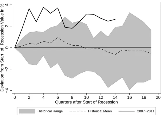
Figure 1 Personal Saving Rate in 2007–2011 and Previous Recessions −4 −2 0 2 4
Deviation from Start−of−Recession Value in %
0 2 4 6 8 10 12 14 16 18 20
Quarters after Start of Recession
Historical Range Historical Mean 2007−2011
Notes: The saving rate is expressed as a percent of disposable income. The figure shows the deviation from its value at the start of recession in percentage points. Historical Range includes all recessions after 1960Q1.
Sources: U.S. Department of Commerce, Bureau of Economic Analysis.
1 Introduction
Fresh interest in the determinants of personal saving has recently been sparked by the remarkable saving rise during the Great Recession:1 For the three years after the
business cycle peak in 2007, the U.S. saving rate has remained substantially above its pre-crisis value, and the increase relative to its 2007 value generally exceeded the maximum saving increase after any previous postwar business cycle peak (see Figure 1).
1We focus on the U.S. because of its central role in triggering the global economic crisis, and because of the rich existing literature studying U.S. data, but the U.K., Ireland, and many other countries also saw substantial increases in personal saving rates.
Abiad, Mathias Hoffmann, Charles Kramer, María Luengo-Prado, Bartosz Maćkowiak, John Muellbauer, David Robinson, Jonathan Wright and seminar audiences at the Bank of England, the ECB and the 2011 NBER Summer Institute for insightful comments. We are grateful to John Duca and John Muellbauer for sharing with us their data on credit conditions. The views presented in this paper are those of the authors, and should not be attributed to the International Monetary Fund, its Executive Board, or management, or to the European Central Bank.
Carroll (1992) invoked precautionary motives to explain the tendency of saving to increase during recessions, showing that an older modeling tradition that had emphasized the role of “wealth effects”2 did not capture cyclical dynamics adequately
(particularly for the first of the ‘postmodern’ recessions in 1990–913
when wealth changed little but saving and unemployment expectations rose markedly).
A largely separate literature has addressed another longstanding saving puzzle: The steady decline in the U.S. personal saving rate, from over 10 percent of disposable income in the early 1980s to a mere 1 percent in the mid-2000s;4 here, a prominent
theme has been the role of financial liberalization in making it easier for households to borrow. (SeeParker (2000) for a comprehensive analysis). Some very recent work (Guerrieri and Lorenzoni (2011), Eggertsson and Krugman (2011), Hall (2011)) has argued (though without much attempt at quantification) that a sudden sharp reversal of this credit-loosening trend played a large role in the recent saving rise.
This paper aims to quantify these three channels, both over the longer span of historical experience and for the period since the beginning of the Great Recession.
To fix ideas, the paper begins by presenting (in section 2) a stylized ‘buffer stock’ saving model with explicit and transparent roles for each of the influences emphasized above (the precautionary, wealth, and credit channels). The model’s key intuition is that, in the presence of income uncertainty, optimizing households have a target wealth ratio that depends on the usual theoretical considerations (risk aversion, time preference, expected income growth, etc), as well as on two features that have been harder to fit into simple stylized models: The degree of labor income uncertainty and the availability of credit. Our model provides a tractable analytical formulation that can be used to calibrate how much saving should go up in response to an increase in uncertainty, or a negative shock to wealth, or a tightening of liquidity constraints.
We highlight one particularly interesting implication of the model: In response to a permanent worsening in economic circumstances (such as a permanent increase in unemployment risk), consumption initially ‘overshoots’ its ultimate permanent adjustment. This reflects the fact that, when the target level of wealth rises, not only is a higher level of steady-state saving needed to maintain a higher target level of wealth, an immediate further boost to saving is necessary to move from the current (inadequate) level of wealth up to the new (higher) target. An interesting implication is that if the economy suffers from adjustment costs for overall aggregate demand (as macroeconomic models strongly suggest), it might be optimal for the government to engage in policies designed to counteract the component of the consumption decline that reflects ‘overshooting.’ In an economy rendered non-Ricardian by the presence
2SeeDavis and Palumbo(2001) for an exposition, estimation, and review.
3Krugman(2012) coined the term ‘postmodern’ to capture the change in the pattern of business cycle dynamics
dating from the 1990–91 recession (particularly the slowness of employment to recover compared to output). But the pattern has been noted by many other macroeconomists.
4Although NIPA accounting conventions impart an inflation-related bias to the measurement of personal saving, the downward trend in saving remains obvious even in an inflation-adjusted measure of the saving rate.
of liquidity constraints and/or uncertainty, this provides a potential rationale for countercyclical fiscal policy, either targeted at households or to boost components of aggregate demand other than household spending in order to offset the temporary downward overshooting of consumption.
After section 3’s discussion of data and measurement issues, section 4 presents an empirical model, motivated by the theory, that attempts to measure the relative importance of each of these effects (precautionary, wealth, and credit) for the U.S. personal saving rate. An OLS regression of the personal saving rate on proxies for the model’s three variables finds a statistically significant and economically important role for all three.
Section 5 of the paper constructs a more explicit relationship between the theo-retical model and the empirical results, by making a direct identification between the model’s parameters (like unemployment risk) and the corresponding empirical objects (like households’ unemployment expectations constructed using the Thomson Reuters/University of Michigan’s Surveys of Consumers). We show that the structural model fits the data essentially as well as the reduced form model, but with the usual advantage of structural models that it is possible to use the estimated model to provide a disciplined investigation of quantitative theoretical issues such as whether there is an interaction betewen the precautionary motive and credit constraints. (We find some evidence that there is).
2 Theory: Target Wealth and Credit Conditions
Carroll and Toche(2009) (henceforth CT) provide a tractable framework for analyzing the impact of nonfinancial uncertainty, in the specific form of unemployment risk, on optimal household saving. The consumer maximizes the discounted sum of utility from an intertemporally separable CRRA utility function u(•) =•1−ρ/(1−ρ)subject to the dynamic budget constraint:
mt+1 = (mt−ct)R+`t+1Wt+1ξt+1,
where next period’s market resources mt+1 are the sum of current market resources net of consumption ct, augmented by the (constant) interest factor R = 1 +r, and with the addition of labor income. The level of labor income is determined by the individual’s productivity`(lower case letters designate individual-level variables), the (upper-case) aggregate wageWt+1 (per unit of productivity) and a zero–one indicator of the consumer’s employment status ξ.
The key feature that makes the model tractable is the assumption that unem-ployment risk takes a particularly stark form: Employed consumers face a constant probability 0 of becoming unemployed; and, once unemployed, the consumer can
never become employed again.5
Under these assumptions, CT show that the steady-state target wealthmˇ depends on unemployment risk0, the interest rater, the growth rate of wages∆W, relative risk aversion ρ, and the discount factor β:6
ˇ m=f(0 (+) , r (+),∆(−W) , ρ(+) , β (+) ). (1)
Target wealth increases with unemployment risk, because in response to higher uncer-tainty, consumers choose to build up a larger precautionary buffer of wealth to protect their spending. (The increase in0is a pure increase in risk (a mean-preserving spread in human wealth) because productivity is assumed to grow by the factor 1/(1−0) each period,`t+1 =`t/(1−0)(see Carroll and Toche(2009), p. 6)). A higher interest rate increases the rewards to holding wealth and thus increases the amount held. Faster income growth translates into a lower wealth target because households who anticipate higher future income consume more now in anticipation of their future prosperity (the ‘human wealth effect’). Finally, risk aversion and the discount factor have effects on target wealth that are qualitatively similar to the effects of uncertainty and the interest rate, respectively. While the unemployment risk inCarroll and Toche
(2009) is of a simple form, the key mechanisms at work are the same as those in more sophisticated setups with a realistic specification of uninsurable risks (building on the work of Skinner (1988),Zeldes (1989),Deaton (1991),Carroll (1997) and others).
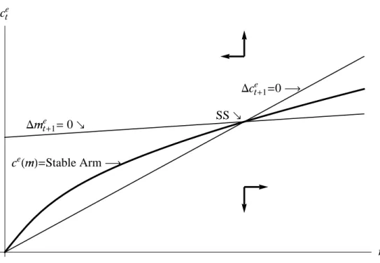
Figure 2shows the phase diagram for the CT model. The consumption function is indicated by the thick solid locus, which is the saddle path that leads to the steady state at which the ratios of both consumption and market resources to income (cand
m) are constant.7
This consumption function can be used directly to analyze the consequences of an exogenous shock to wealth of the kind contemplated in the old “wealth effects” literature, or in the AEA Presidential address of Hall(2011).8 The consequences of a
5Of course, if a starting population of such consumers were not refreshed by an inflow of new employed consumers, the unemployment rate would asymptote to 100 percent. This problem can easily be addressed by introducing simple demographics (which do not affect the optimization problem of the employed): Each period new employed consumers are born and a fraction of existing households dies, as inCarroll and Jeanne(2009). Because demographic effects are very gradual, the implications of the more complicated model are well captured by the simpler model presented here that ignores demographics and the behavior of the unemployed population.
6Specifically, the steady-state target wealth can be approximated as
ˇ m= 1 + 1 þr( ˆpγ/0)−þγ , whereþr= log (Rβ)1/ρ R,þγ= log (Rβ)1/ρ Γ,ˆþγ=þγ(1 +þγω/0),Γ = (1 + ∆W)/(1−0)andω= (ρ−1)/2.
7For a detailed intuitive exposition of the model, see
http://econ.jhu.edu/people/ccarroll/public/lecturenotes/consumption/tractablebufferstock/.
8Like that literature, we take the wealth shock to be exogenous. It is clear from the prior literature starting with
Merton(1969) andSamuelson(1969) that not much would change if a risky return were incorporated and the wealth
shock were interpreted as a particularly bad realization of the stochastic return on assets. The much more difficult problem of constructing a plausible theory of endogenous asset pricing that could justify the observed wealth shocks has not yet been satisfactorily solved, which is whyHall(2011) treated the wealth shocks at the beginning of the Great Recession as exogenous.
Dcte+1= 0 Dmte+1= 0 ceHmL=Stable Arm SS mte cte
Figure 2 Consumption Function (Stable Arm of Phase Diagram)
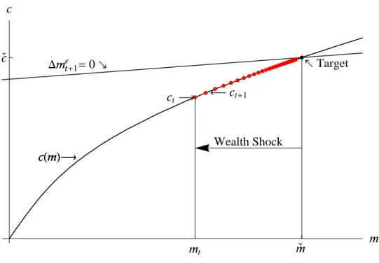
pure shock to wealth are depicted in figure 3 and are straightforward: Consumption declines upon impact, to a level below the value that would leave me constant (the leftmost red dot); because consumption is below income, me (and thus ce – the sequence of red dots) rises over time back toward the original target.
The model solved in CT deliberately omitted explicit liquidity constraints in order to emphasize the conceptual point that uncertainty induces concavity of the con-sumption function (that is, a higher marginal propensity to consume for people with low levels of wealth) even in the absence of constraints (for a general proof of this proposition, seeCarroll and Kimball(1996)). Indeed, because the employed consumer is always at risk of a transition into the unemployed state where income will be zero, the ‘natural borrowing constraint’ in this model prevents the consumer from ever choosing to go into debt, because an indebted unemployed consumer with zero income might be forced to consume a negative amount to satisfy the budget constraint.
We make only one modification to the CT model for the purpose at hand: We introduce an ‘unemployment insurance’ system that guarantees a positive level of income for unemployed households. In the presence of such insurance, households with low levels of market resources will be willing to borrow because they will not starve even if they become unemployed. The effect of this change is simply to induce a leftward shift in the consumption function by an amount corresponding to the present discounted value of the unemployment benefit. The consumer will limit his indebtedness, however, to an amount small enough to guarantee that consumption will
Dmte+1=0 cHmL ct ct+1 Wealth Shock Target cHmL mÇ mt m cÇ c
Figure 3 A Wealth Shock
remain strictly positive even when unemployed (this requirement defines the ‘natural borrowing constraint’ in this model).
We could easily add a tighter ‘artificial’ liquidity constraint, imposed exogenously by the financial system, that would prevent the consumer from borrowing as much as the natural borrowing constraint permits. But Carroll (2001) shows that the effects of tightening an artificial constraint are qualitatively and quantitatively similar to the effects of tightening the natural borrowing constraint; while we do not doubt that artificial borrowing constraints exist and are important, we do not incorporate them into our framework since we can capture their consequences by manipulating the natural borrowing constraint that is already an intrinsic element of the model. Indeed, using this strategy, our empirical estimates below will interpret the process of financial liberalization which began in the U.S. in the early 1980s and arguably continued until the eve of the Great Recession as the major explanation for the long downtrend in the saving rate.
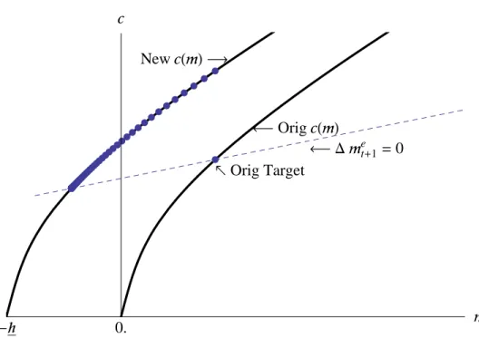
Figure4shows that the model reproduces the standard result from the existing lit-erature (see, e.g.,Carroll(2001),Muellbauer (2007),Guerrieri and Lorenzoni(2011),
Hall(2011)): Relaxation of the borrowing constraint (from an inital position of 0. in which no borrowing occurs, to a new value in which the natural borrowing limit is h
implying minimum net worth of−h) leads to an immediate increase in consumption for a given level of resources. But over time, the higher spending causes the consumer’s level of wealth to decline, forcing a corresponding gradual decline in consumption
Orig Target Dmte+1=0 OrigcHmL NewcHmL -h 0. m c
Figure 4 Relaxation of a Natural Borrowing Constraint from 0. to h
until wealth eventually settles at its new, lower target level. (For vivid illustration, parameter values for this figure were chosen such that the new target level of wealth is negative; that is, the consumer would be in debt, in equilibrium).
Rather presenting yet another variant of the phase diagram, we instead illustrate our next experiment by showing the dynamics of the saving rate rather than the level of consumption over time. (Since both saving and consumption are strictly monotonic functions of me, there is a strict equivalence between the two ways of presenting the results).
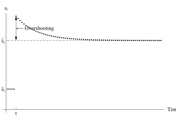
Figure5 shows the consequences of a permanent increase in unemployment risk0: An immediate jump in the saving rate, followed by a gradual decline toward a new equilibrium rate that is higher than the original one.
Qualitatively, the effects are essentially the opposite of a credit loosening: In response to a human-wealth-preserving spread in unemployment risk, the level of consumption falls sharply as consumers begin the process of accumulation toward a higher target wealth ratio.9 This figure vividly illustrates the ‘overshooting’
proposi-tion menproposi-tioned in the introducproposi-tion: All of the initial increase in saving reflects a drop in consumption (by construction, the mean-preserving spread in unemployment risk 9The model is specified in such a way that an increase in the parameter0that we are calling the ‘unemployment risk’ here actually induces an offsetting increase in the expected mean level of income (an increase in0is a mean-preserving spread in the relevant sense); the spending of a consumer with certainty-equivalent preferences therefore would not change in response to a change in0, so we can attribute all of the increase in the saving rate depicted in the figure to the precautionary motive.
Overshooting t Time sÇt sÇt ' st
Figure 5 Dynamics of the Saving Rate after an Increase in Unemployment Risk
leaves current income unchanged), and consumption recovers only gradually toward its ultimately higher target. For a long time, the saving rate remains above either its pre-shock level or its new target. While the implications for optimal fiscal policy are beyond the scope of our analysis, it is clear that a number of policies could either mitigate the consumption decline (e.g., an increase in social insurance) or replace the corresponding deficiency in aggregate demand (e.g., by an increase in government spending). We leave further exploration of these ideas to later work, or other authors. One objection to the model might be that its extreme assumption about the nature of unemployment risk (once unemployed, the consumer can never become reemployed) calls into question its practical usefulness except as a convenient stylized treatment of the logic of precautionary saving. Our view is that such a criticism would be misplaced, for several reasons. First, when unemployment risk in the model is set to zero, it collapses to the standard Ramsey model that has been a workhorse for much of macroeconomic analysis for the past 40 years (see Carroll and Toche(2009) for details). It seems perverse to criticize the model for moving at least a step in the direction of realism by introducing a precautionary motive into that framework. Second, this paper’s authors have been active participants in the literature that builds far more empirically realistic models of precautionary saving, but our considered judgment is that in the present context the virtues of transparency and simplicity far outweigh the model’s cost in realism. Models are metaphors, not high-definition photographs, and if a certain flexibility of interpretation is granted to use a simple
model that has all the right parts, more progress might be made than by building a state-of-the-art Titanic.
In sum, the model emphasizes three factors that affect saving and that might vary substantially over time. First, because the precautionary motive diminishes as wealth rises, the saving rate is a declining function of market resources mt. Second, since an expansion in the availability of credit reduces the target level of wealth, looser credit conditions (designated CEAt, for reasons articulated below) lead to lower saving. Finally, higher unemployment risk 0t results in greater saving for precautionary reasons.
The framework thus suggests that a reduced-form regression for the saving ratest
st =γ0+γmmt+γCEACEAt+γ00t+γ0Xt+εst (2) should satisfy the following conditions:
γm <0, γCEA <0, γ0 >0, (3)
where CEAtdenotes the “Credit Easing Accumulated” index, a measure of credit sup-ply (described in detail below), and the vectorXt collects other drivers of saving that are outside the scope of the model, such as demographics, corporate and government saving, etc. We estimate regressions of the form (2) in section4 below.
To economists steeped in the wisdom of IrvingFisher(1930) according to whom the consumption path is determined by lifetime resources independently of the income path (‘Fisherian separation holds’), equation (2) may seem like a throwback to the bad old days of nonstructural Keynesian estimation of the kind that fell into ill repute after spectacular failures in the 1970s. Below, however, we will show that, at least under our assumptions, a reduced form estimation of such an equation can in principle yield estimates of “structural” parameters like the time preference rate. (An important part of the reason this excercise is not implausible is that, with the exception of a few easily identified episodes, the growth rate of personal income is not very far from a random walk with drift, justifying the identification of actual income with ‘permanent income’ in a Friedmanian sense).10
3 Data and Measurement Issues
Before presenting estimation results we introduce our dataset. Because our empirical measure of credit conditions begins in 1966q2, our analysis begins at that date and 10More precisely, an empirical decomposition of NIPA personal disposable income into permanent and transitory components (in which income consists of unobserved random walk with drift and white noise) assigns almost all variation in (measured) income to its permanent component, so that a ratio to actual income will coincide almost perfectly with a ratio to estimated ‘permanent’ income. This is not surprising because, as is well-known (and also documented in Appendix 2), it is difficult to reject the proposition that almost all shocks to the level of aggregate income are permanent; autocorrelation functions and partial autocorrelation functions indicate that log-level of disposable income is close to a random walk; see our further discussion in Appendix 2.
extends (at the present writing) through 2011q1.11,12
The saving rate is from the BEA’s National Income and Product Accounts and is expressed as a percentage of disposable income.13,14
One objection to our analysis might be that some items that are included in personal consumption expenditures (in particular, spending on highly durable goods like automobiles) are more properly treated as saving in a nonfinancial form rather than spending. We acknowledge this point, but our view is that its force is easily exaggerated, for several reasons. Perhaps the most important is that in the short run, the most urgent purpose for modeling of this kind is to provide guidance to policymakers who need to assess the likely path of consumer expenditures as defined in the national accounts, since such direct spending is what contributes to GDP and can be influenced by both fiscal and monetary policy. Policymakers who were offered a model that fitted ‘consumption’ as abstractly defined by theory, but did not say much about NIPA PCE, would probably prefer our model. A second response is that, with respect to long-run trends, the depreciation rate of durable goods included in NIPA PCE (even including automobiles) is high enough that we would not expect much bias from the ‘durables’ problem over the course of a 45 year estimation period. A further point is that the theoretical forces in which we are most interested, the roles of liquidity constraints and precautionary saving, are precisely those forces that have been shown most seriously to undermine the implications of the intellectual framework (perfect foresight, perfect capital markets, no adjustment costs, etc) that justifies the treatment of automobile purchases as equivalent to saving in a drivable investment vehicle. Finally, any attempt to perform an analysis similar to ours but using a more theoretically “pure” measure of consumption quickly descends into a morass of arbitrary judgments like whether spending on holiday travel is “durable” because memories can last a lifetime. While some existing papers have made a stab at drawing such lines, our view is that at the quarterly frequency probably the only
11Most time series were downloaded from Haver Analytics, and were originally compiled by the Bureau of Economic Analysis, the Bureau of Labor Statistics or the Federal Reserve.
12We are reluctant to use more recent data because personal saving rate statistics are subject to large revisions; see the insightful analysis inDeutsche Bank Securities(2012), showing that preliminary U.S. income and saving rate data are systematically revised upward when full data become available.
13As a robustness check, we have also re-estimated our models with alternative measures of saving: Gross household saving as a fraction of disposable income, gross and net private saving as a fraction of GDP, inflation-adjusted personal saving rate and two measures of saving from the Flow of Funds (with/without consumer durables). The inflation-adjusted saving rate deducts from saving the erosion in the value of money-denominated assets due to inflation. The Flow of Funds (FoF) calculates saving as the sum of the net acquisition of financial assets and tangible assets minus the net increase in liabilities. Because this FoF-based measure is substantially more volatile, the fit of the model is worse than for the NIPA-based PSR. However, the main messages of the paper remain unchanged.
14Many reasonable objections can be made to this, or any other, specific measure of the personal saving rate, including the treatment of durable goods, the treatment of capital gains and losses, and so on. While some defense of the NIPA measure could be made in response to many of these challenges, such defenses would take us too far afield, and we refer the reader to the extensive discussions of these measurement issues that date at least back toFriedman (1957).
goods that are pretty clearly nondurable are fresh fruits and vegetables. (Canned ones can last much longer than a quarter, and even meat and fish can be frozen).
Market resourcesmtare measured as the ratio of household net worth to disposable income, in line with the model.15
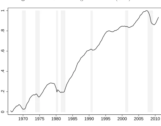
Our measure of credit supply conditions, which we call the Credit Easing Accumulated index (CEA, see Figure 6) is constructed in the spirit of Muellbauer (2007) and Duca, Muellbauer, and Murphy (2010) using the question on consumer installment loans from the Federal Reserve’s Senior Loan Officer Opinion Survey (SLOOS) on Bank Lending Practices (see also Fernandez-Corugedo and Muellbauer (2006) and Hall (2011)). The question asks about banks’ willingness to make consumer installment loans now as opposed to three months ago. To calculate a proxy for the level of credit conditions, the scores from the survey were accumulated, weighting the responses by the debt–income ratio to account for the increasing trend in that variable.16
(The index is normalized between 0 and 1 to make the interpretation of regression coefficients straightforward.)
The CEA index is taken to measure the availability/supply of credit to a typical household through factors other than the level of interest rates—for example, through loan to value and loan to income ratios, availability of mortgage equity withdrawal and mortgage refinancing. The broad trends in the CEA index correlate strongly with measures financial reforms of Abiad, Detragiache, and Tressel (2008), and measures of banking deregulation of Demyanyk, Ostergaard, and Sørensen (2007) (see panel A of their Figure 1, p. 2786).17 In addition, they seem to reflect well the key
developments of the U.S. financial market institutions as described in McCarthy and Peach (2002), Dynan, Elmendorf, and Sichel (2006), Green and Wachter (2007), and Campbell and Hercowitz (2009), among others. Until the early 1980s, the U.S. consumer lending markets were quite heavily regulated and segmented. After the phaseout of interest rate controls beginning in the early 1980s, the markets became more competitive, spurring financial innovations that led to greater access to credit. Technological progress leading to new financial instruments and better credit screening methods, a greater role of nonbanking financial institutions, and the increased use of securitization all contributed to the dramatic rise in credit availability from the early 1980s until the onset of the Great Recession in 2007. The subsequent significant drop in the CEA index was associated with the funding difficulties and de-leveraging of financial institutions. As a caveat, it is important to acknowledge that CEA might to some degree be influenced by developments from the demand rather 15This variable is lagged by one quarter to account for the fact that data on net worth are reported as the end-of-period values.
16As inMuellbauer (2007), we use the question on consumer installment loans rather than mortgages because the latter is only available starting in 1990Q2 and the question changed in 2007Q2. Our CEA index differs from
Muellbauer(2007)’s Credit Conditions Index in that Muellbauer accumulates raw answers, not weighting them by the
debt–income ratio.
17Duca, Muellbauer, and Murphy(2011) document an increasing trend in loan to value ratios for first-time home
buyers (in data from the American Housing Survey, 1979–2007), an indicator which is arguably to some extent affected by fluctuations in demand.
Figure 6 The Credit Easing Accumulated (CEA) Index 0 .2 .4 .6 .8 1 1970 1975 1980 1985 1990 1995 2000 2005 2010 Notes: Shading—NBER recessions.
Sources: Federal Reserve, accumulated scores from the question on change in the banks’ willingness to provide consumer installment loans from the Senior Loan Officer Opinion Survey on Bank Lending Practices,
Figure 7 Unemployment Risk Etut+4 and Unemployment Rate (Percent) 2 4 6 8 10 1970 1975 1980 1985 1990 1995 2000 2005 2010
Legend: Unemployment rate: Thin black line, Unemployment risk Etut+4: Thick red/grey line. Shading—NBER recessions.
Sources: Thomson Reuters/University of Michigan Surveys of Consumers,http://www.sca.isr.umich.edu/main.php, Bureau of Labor Statistics.
than the supply side of the credit market. But whatever its flaws in this regard, indexes of this sort seem to be gaining increasing acceptance as the best available measures of credit supply (as distinguished from credit demand).18
We measure a proxy Etut+4 for unemployment risk 0t using re-scaled answers to the question about the expected change in unemployment in the Thomson Reuters/University of Michigan Surveys of Consumers.19 In particular, we estimate
Etut+4 using fitted values ∆4uˆt+4 from the regression of the four-quarter-ahead change in unemployment rate ∆4ut+4 ≡ ut+4 − ut on the answer in the survey,
18We have verified that our results do not materially change when we use the credit conditions index ofDuca,
Muellbauer, and Murphy(2010), which differs from our CEA in thatDuca, Muellbauer, and Murphyexplicitly remove
identifiable effects of interest rates and the macroeconomic outlook from the SLOOS data using regression techniques. Since the results are similar using both measures, our interpretation is that our measure is at least not merely capturing the most obvious cyclical components of credit demand. As reported below, our results also do not change when we use the Financial Liberalization Index ofAbiad, Detragiache, and Tressel(2008)—which is based on the readings of financial laws and regulations—as an instrument for CEA.
19The relevant question is: “How about people out of work during the coming 12 months—do you think that there will be more unemployment than now, about the same, or less?”
summarized with a balance statistic UExpBSt :
∆4ut+4 = α0+α1UExpBSt +εt+4, Etut+4 = ut+ ∆4uˆt+4.
The coefficient α1 is highly statistically significant (indicating that households do have substantial information about the direction of future changes in the unem-ployment rate). Our Etut+4 series, which—as expected—correlates strongly with unemployment rate and precedes its dynamics, is shown in Figure 7.
4 Reduced-Form Saving Regressions
Before proceeding to structural estimation of the model of section 2we investigate a simple reduced-form benchmark:
st=γ1+γmmt+γCEACEAt+γEuEtut+4+γtt+γ0Xt+εst. (4) Such a specification can be readily estimated using OLS or IV estimators, and at a minimum can be interpreted as summarizing basic stylized facts about the data.
Table 1 reports the estimated coefficients from several variations on equation (4). The first four columns show univariate specifications in which the saving rate is in turn regressed on each of the three determinants analyzed above: Wealth, credit conditions, and unemployment risk. In each specification we include the time trend to investigate how much each regressor contributes to explaining the PSR beyond the portion that can be captured mechanically by a linear time effect. The three coefficients have the signs predicted by the model of section 2 and are statistically significant. Univariate regressions capture up to 85 percent of variation in saving.
But the univariate models on their own do not adequately describe the dynamics of the PSR. As the model labeled “All 3” in the fifth column shows, the three key variables of interest—wealth and credit conditions—jointly explain roughly 90 percent of the variation in the saving rate over the past five decades. As expected, the point estimates again indicate a strong negative correlation between saving and net wealth and credit conditions and a positive correlation with unemployment risk. Interestingly, once the three variables are included jointly, the time trend ceases to be significant, which is in line with the fact that the three models in columns 2–4 have higher R¯2 that the univariate model with the time trend only.20
The specification in column 5 (All 3) suggests that a more parsimonious version of the model without the time trend reported in column 6 (Baseline)—and also suggested by the structure of section 2—neatly summarizes the key features of the 20Estimating univariate saving regressions without the time trend, results in higherR¯2for wealth and the credit conditions—0.72 and 0.80, respectively—that for the “time” model in column one (0.70). (Because unemployment risk is not trending, it captures relatively little variation in saving on its own (about 10 percent) but is importantin additionto the two other factors, as illustrated in columns 4 and 5.)
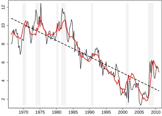
Figure 8 The Fit of the Baseline Model and the Time Trend—Actual and Fitted Saving Rate 2 4 6 8 10 12 1970 1975 1980 1985 1990 1995 2000 2005 2010
Legend: Actual PSR: Thin black line, Baseline model: Thick red/grey line, Time trend: Dashed black line. Shading—NBER recessions.
saving rate. The estimated coefficient on net wealth implies the (direct) long-run marginal propensity to consume of about 1.2 cents out of a dollar of (total) wealth. The value is low compared to much of the literature, which typically estimates a marginal propensity to consume out of wealth (MPCW) of about 3–7 cents without explicitly accounting for credit conditions.21 However, a univariate model regressing
the PSR just on net wealth (not reported here), implies an MPCW of 4.3 percent. These results suggest that much of what has been interpreted as pure “wealth effects” in the prior literature may actually have reflected precautionary or credit availability effects that are correlated with wealth.
The coefficient on the Credit Easing Accumulated index is highly statistically significant with a t statistic of −10.7. The point estimate of γCEA implies that increased access to credit during the sample period ending in 2007 (before the Great Recession) reduced the PSR by about 6 percentage points of disposable income. In the aftermath of the Recession, the CEA index declined between 2007 and 2010 by roughly 0.11 as credit supply tightened, contributing roughly 0.64 percentage point to the increase in the PSR (see the discussion of Table 3 below for more detail).
Figure 8 further illustrates why we find the “baseline” specification in column 6 more appealing than the more atheoretical model with a linear time trend. The trends in saving and the CEA are both non-linear, moving consistently with each other even within our sample and often persistently departing from the linear trend (as documented also by its substantially lower R¯2). In addition, it is likely that the time-only model will become increasingly problematic as observations beyond our sample accumulate, arguably providing additional evidence on the structural break in the time model during the Great Recession.22
Finally, the last model investigates the joint effect of credit conditions and un-employment risk. The structural model of section 2 implies that uncertainty affects saving more strongly when credit constraints bind tightly; the model in column 7 (Interact) confirms the prediction with a (borderline) significant negative interaction term between the CEA and unemployment risk.23
Table 2 presents a second battery of specification checks of the baseline model (shown again for reference in the first column). The second model (Uncertainty) investigates the effects of adding to the baseline regression an alternative proxy for uncertainty: the Bloom, Floetotto, and Jaimovich (2009) index of macroeconomic and financial uncertainty.24
The new variable is statistically insignificant and the 21See, for example,Skinner(1996),Ludvigson and Steindel(1999),Lettau and Ludvigson(2004),Case, Quigley,
and Shiller (2005), andCarroll, Otsuka, and Slacalek (2011). See Muellbauer (2007) and Duca, Muellbauer, and
Murphy(2010) for a model which includes a measure of credit conditions in the consumption function.
22Reliable PSR data only start in 1959 and document that the downward trend in saving started around 1975, so that our sample is actually quite favorable to the time-only model; it would have considerably more difficulty with a sample that included 10 presample years without a discernable trend.
23Adding an interaction term between the CEA and wealth results in a borderline significant positive estimate, which is in line with the concavity of the consumption function, show in Figure2.
coefficients on the previously included variables are broadly unchanged, suggesting that our baseline uncertainty measure is more appropriate for our purposes (which makes sense, as personal saving is conducted by persons, whose uncertainty is likely better captured by our measure of labor income uncertainty than by the Bloom, Floetotto, and Jaimovich (2009) measure of firm-level shocks).
The third model (Lagged st−1) explores the implications of adding lagged saving to the list of regressors. Somewhat unusually, in the case of our model such serial correlation is not an embarrassing feature of the data that must be acknowledged with averted eyes, but instead is a direct implication of the model. The implication arises because deviations of actual wealth from target wealth ought to be long-lasting if the saving rate cannot quickly move actual wealth toward the target. As expected, coefficient is highly statistically significant. However, this positive autocorrelation only captures near-term stickiness and has little effect on the long-run dynamics of saving. Indeed, the coefficients from the baseline roughly equal their long-term counterparts from the model with lagged saving rates (that is, coefficient estimates pre-multiplied by 2.5, or 1/(1−γs) = 1/(1−0.60)).25
The fourth model (Debt) explores the role of the debt–income ratio. The variable could be relevant for two reasons. First, it could partly account for the fact that debt is held by a different group of people than assets and consequently net worth might be an insufficient measure of wealth. Second, debt might also reflect credit conditions (although—as mentioned above—we prefer the CEA index because in principle it isolates the role of credit supply from demand). The regression can thus also be interpreted as a horse-race between the CEA and the debt–income ratio. In any case, while the coefficient γd has the correct (negative) sign, it is statistically insignificant and its inclusion does not substantially affect estimates obtained under the baseline specification.
The fifth model (Full Controls) controls for the effects of other potential determi-nants of household saving: expected real interest rates, expected income growth, and government and corporate saving (both measured as a percent of GDP).26
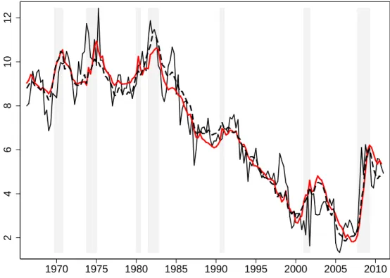
Some of these factors are statistically significant, but all are inconsequential in economic terms. Figure 9makes it clear that while these additional factors were potentially important during specific episodes (especially in the early 1980s), they have on average had only a limited impact on U.S. household saving. The negative coefficient on corporate saving is consistent with the proposition that households may ‘pierce the corporate veil’ to some extent27
but there is no evidence for any interaction between personal and government saving. One interpretation of this is that ‘Ricardian’ effects that 25Note that with the inclusion of lagged saving, the Durbin–Watson statistic becomes close to 2, suggesting that whatever serial correlation exists in the other specifications reflect simple first order autocorrelation of the errors.
26Expected real interest rates and expected income growth are constructed using data from the Survey of Professional Forecasters of the Philadelphia Fed.
27Regressions with total private saving as a dependent variable yield qualitatively similar results as our baseline estimates in Table1.
Figure 9 The Fit of the Baseline Model and the Model with Full Controls (of Table 2)—Actual and Fitted PSR
2 4 6 8 10 12 1970 1975 1980 1985 1990 1995 2000 2005 2010
Legend: Actual PSR: Thin black line, Baseline model: Thick red/grey line, Model with full control variables: Dashed black line. Shading—NBER recessions.
some prior researchers have claimed to find might instead reflect reverse causality: Recessions cause government saving to decline at the same time that personal sav-ing increases (high unemployment, fallsav-ing wealth, restricted credit) but for reasons independent of the Ricardian logic (reduced tax revenues and increased spending on automatic stabilizers, e.g.). Since we are controlling directly for the variables (wealth, unemployment risk, credit availability) that were (in this interpretation) proxied by government saving, we no longer find any effect of government saving on personal saving.
When the model is estimated only using the post-1980 data in the sixth column (Post-1980), its fit measured by the R¯2 actually improves, in contrast with many other economic relationships, whose goodness-of-fit deteriorated in the past 20 years. The F test is consistent with the proposition that the coefficients of the regression have not changed over the sample.
Finally, to explore how much endogeneity may matter,28 the specification “IV”
re-estimates the baseline specification using the IV estimator. Instruments are the lags of net wealth, unemployment risk and—crucially—the Financial Liberalization Index of Abiad, Detragiache, and Tressel (2008) (described in Appendix 1). The FLI is an alternative measure of credit conditions constructed using the records about legal and regulatory changes in the banking sector. The index intends to capture exogenous changes in credit conditions. While it is a rough approximation as it reflects only the most important events (see also Figure 14in Appendix 1), the profile of the FLI matches well that of the CEA. The estimated coefficients remain broadly unchanged compared with the baseline specification.
We have also estimated specifications with other variables, whose detailed results we do not report. As in Parker (2000), demographic variables, like the old-age dependency ratio, were insignificant in our regressions. The importance of population aging in cross–country studies of household saving (for example, Bloom, Canning, Mansfield, and Moore (2007) and Bosworth and Chodorow-Reich(2007)) appears to be largely driven by the experience of Japan and Korea—countries well ahead of the United States in the population aging process.
To address a potential criticism that saving rate regressions are difficult to interpret because aggregate income shocks reflect a mix of transitory and persistent factors, we have also re-estimated our regressions with alternative measures of disposable income (see Appendix 2) which exclude a range of identifiable temporary shocks such as fiscal stimulus and extreme weather. There was little econometric evidence that transitory
28As mentioned above, wealth is lagged by one quarter to alleviate endogeneity in OLS regressions. However, a standard concern about reduced-form regressions like (4) is that the OLS coefficient estimates might be biased because the regressions do not adequately account for all relevant right-hand size variables (such as expectations about income growth; see also Appendix 2 for further discussion).
movements in aggregate disposable income are substantial and our econometric results basically did not change.29
Table3reports in-sample fit of the baseline model and the model Interact with the CEA–uncertainty interaction term of Table 1, and the contributions of the individual variables to the explained increase in the saving rate between 2007 and 2010. Two principal conclusions emerge. First, both models (especially the latter) are able to capture well the observed change in the saving rate. Second, the key explanatory factors in saving over the past two years were the changes in wealth and uncertainty, with credit conditions (as measured by CEA) playing a less important role. While the change in the trajectory of the CEA index is quite striking (see Figure 6), and may explain the sudden academic interest in the role of household credit over the business cycle (see the papers cited in the introduction), this evidence suggests that the rise in saving cannot be mainly attributed to the decline in credit availability. If correct, this finding is particularly important at the present juncture because it suggests that however much the health of the financial sector continues improving, the saving rate is likely to remain high so long as uncertainty remains high and household wealth remains impaired (compared, at least, to its previous heights).
5 Structural Estimation
This section estimates the structural model of section 2 by minimizing the distance between the data on saving implied by the model and those observed in reality. The nonlinear least squares (NLLS) procedure we use has some advantages over the reduced-form regressions. Besides arguably being more immune to endogeneity and suitable for estimating structural parameters (such as the discount factor), it imposes on the data a structure that makes them easier to interpret. In particular, the model identifies a value for target wealth, which varies depending on the evolution of risk and credit conditions, and which can in principle be useful for identifying major deviations of actual wealth from the optimal level desired by consumers and gauging future trends in the saving rate. As Figure 2 documents, the structural model explicitly justifies and disciplines non-linearities, which can be important especially during turbulent times, when the shocks are large enough to move the system far from its steady state. In such times, estimation of linear or linearized models may be subject to substantial error.
29Interestingly, an auxiliary regression of income growth on the lagged saving rate in the spirit ofCampbell(1987) yields statistically insignificant slope when post-1985 data are included (see Table7in Appendix 2).
5.1 Estimation Procedure
We assume households instantaneously observe exogenous movements in the three factors: wealth shocks m, unemployment risk 0 and credit supply conditions CEA, and that they consider the shocks to0and CEA to be permanent (and do not expect the shocks to wealth to be reversed).30 Given these factors and the parameters,
each period consumers re-optimize their consumption–saving choice (described in section2). Collecting the parameters in the vector Θand denoting the target wealth
ˇ
mt(·)and the corresponding wealth gapmt−mˇt, the model implies a series of saving rates stheort (Θ;mt−mˇt), which we match to those observed in the data, smeast . Our estimates Θˆ thus solve the following problem:
ˆ Θ = arg min T X t=1 smeast −stheort Θ;mt−mˇ m¯(CEAt),0(Etut+4) 2 , (5)
where the target wealth mˇ depends on the credit conditions and unemployment risk as described in section 2. In our baseline specification the parameter vector Θconsists of the discount factorβ and the scaling constants for credit conditions and unemployment risk:
Θ = {β,θ¯m, θCEA,θ¯0, θu}, (6)
¯
mt = θ¯m+θCEACEAt, (7)
0t = θ¯0+θuEtut+4. (8)
The re-scaling ensures that the unitless measure of credit conditions is re-normalized as a fraction of disposable income and that the expected unemployment rate is transformed into the model-compatible equivalent of permanent risk. The model implies that θCEA >0 and θu >0.
Minimization (5) is a non-linear least squares problem in which the standard asymp-totic results apply. Standard errors for the estimated parameters are calculated using the delta method as follows.31 Define the scores q
t(Θ) = smeast −stheort (Θ) ∂stheor
t (Θ)
∂Θ0
and the 5×5 matrices E = var qt(Θ)
and D = E∂qt(Θ)
∂Θ0 . The estimates have the
asymptotic distribution:
T1/2( ˆΘ−Θ) →dN(0, D−1ED0−1).
30The assumption that households believe the shocks to be permanent is necessary for us to be able to use the tractable model we described earlier in the paper. While indefensible as a literal proposition (presumably nobody believes the unemployment rate will remain high forever), the high serial correlation of these variables means that the assumption may not be too objectionable. In any case, a model that incorporated more realistic descriptions of these processes would be much less transparent and might not be computationally feasible with present technology.
31To construct the objective function (which we then minimize over Θ) we need to solve the consumer’s optimization for each quarter. Because the calculation is computationally demanding, we cannot apply bootstrap to calculate standard errors. (The Shapiro–Wilk test does not reject normality of residuals.)
Because the saving functionstheort (Θ) is not available in the closed form, we calculate its partial derivatives numerically.
5.2 Results
Table 4 summarizes the calibration and the estimation results. The calibrated parameters—real interest rate r = 0.04/4, wage growth ∆W = 0.01/4 and the coefficient of relative risk aversion ρ = 2 take their standard (quarterly) values and meet (together with the discount factor β) the conditions sufficient for the problem to be well-defined.
The discount factorβ = 1−0.0064 = 0.9936, or 0.975 at annual frequency, lies in the standard range.
Figure10shows the estimated horizontal shift in the consumption functionm¯t. The estimates of the scaling factors θ¯m and θCEA imply that m¯t varies roughly between 0 and (−0.0071 + 5.2208)/4 = 1.3, implying that financial deregulation resulted at its peak in an availability of credit in 2007 that was greater than credit availability at the beginning of our sample in 1966 by an amount equal to about 130% of annual income—not an unreasonable figure.
Figure 11 shows the estimated quarterly intensity of perceived permanent unem-ployment risk.
Figure 12 shows the fit of the structural model. In terms of R¯2 (Table 4), the model captures more than 80 percent of variation in the saving rate, doing only slightly worse than our baseline reduced-form model (whose R¯2 is roughly 0.9). The Mincer–Zarnowitz horse race between the models puts roughly 0.45 on the structural model (although the high standard error on the coefficient signals the high correlation between the two model-implied saving rates).
In principle, time variation in the fitted saving rate arises in our model exclusively due to the precautionary motive, which can be broken down into the three compo-nents: uncertainty, wealth, and credit conditions, as shown in Figure 13. Given the estimated parametersΘ(from Table4) we sequentially switch off the uncertainty and credit supply channels by setting the values of these series equal to their sample means. This means that, e.g., the difference between the model fitted series (red/grey line and the fitted series excluding uncertainty (black line) in Figure 13 is to be interpreted as the effects of time variation in unemployment risk 0 (rather than total extent of saving caused by the existence of uncertainty).
While the wealth fluctuations do contribute to a good performance of the model at the business-cycle frequencies, the CEA is essential in capturing the trend decline in the PSR between the 1980s and the early 2000s. The principal role of cyclical fluctuations in uncertainty is to magnify the increases in the PSR during recessions, including the last one.
Figure 10 Extent of Credit Constraints m¯t (Fraction of Quarterly Disposable Income) 1970 1975 1980 1985 1990 1995 2000 2005 2010 0 0.5 1 1.5 2 2.5 3 3.5 4 4.5 5 5.5
Notes: Shading—NBER recessions.
Sources: Federal Reserve, accumulated scores from the question on change in the banks’ willingness to provide consumer installment loans from the Senior Loan Officer Opinion Survey on Bank Lending Practices,
Figure 11 Per Quarter Permanent Unemployment Risk 0t 1970 1975 1980 1985 1990 1995 2000 2005 2010 5.5 6 6.5 7 7.5 8 8.5 9x 10 −5
Notes: Shading—NBER recessions.
Sources: Thomson Reuters/University of Michigan Surveys of Consumers,http://www.sca.isr.umich.edu/main.php, Bureau of Labor Statistics, authors’ calculations.
Figure 12 Fit of the Structural Model—Actual and Fitted PSR 1970 1975 1980 1985 1990 1995 2000 2005 2010 0 2 4 6 8 10 12
Legend: Actual PSR: Thin black line, Structural model: Thick red/grey line. Shading— NBER recessions.
Figure 13 Decomposition of Fitted PSR 1970 1975 1980 1985 1990 1995 2000 2005 2010 0 2 4 6 8 10 12 Fitted PSR
Fitted PSR excl. Uncertainty
Fitted PSR excl. Uncertainty and CEA
Notes: Shading—NBER recessions.
Table 5 replicates the estimates of Table 1 for the (artificial) saving rate series generated by the estimated structural model. The fact that the coefficient estimates closely mirror those obtained in actual time series documents that the structural model captures well key features of the data on saving. Unsurprisingly, the standard errors are somewhat smaller than those in Table 1 and the R¯2s are higher because the process of generating the artificial data by the model eliminates much of the noise (which is present in the actual data on the PSR).
6 Conclusions
We find evidence that credit availability, shocks to household wealth, and movements in income uncertainty have all been important factors in driving U.S. household saving over the past 45 years. In particular, a relentless expansion of credit supply between the mid-1980s and 2007 (likely largely reflecting financial innovation and liberalization), along with higher asset values and consequent increases in net wealth (possibly also partly attributable to the credit boom) encouraged households to save less out of their disposable income. At the same time, the fluctuations in net wealth and labor income uncertainty, for instance during and after the burst of the information technology and credit bubbles of 2001 and 2007, can explain the bulk of business cycle fluctuations in personal saving.
We also find that other determinants of saving suggested by various literatures (e.g., fiscal deficits, demographics, income expectations) either work through the key factors above, are of second-order importance, or matter only during particular episodes. These findings are broadly in line with the complementary household-level evidence reported in Dynan and Kohn (2007), Moore and Palumbo (2010), Bricker, Bucks, Kennickell, Mach, and Moore (2011) andPetev, Pistaferri, and Eksten (2011).32
Of course, all this evidence is based on historical data and, going forward, factors such as rapidly rising federal debt or the retirement of baby-boomers could yet lead to new structural shifts in household saving. From a more conjectural perspective, our results suggest that the personal saving rate in the pre-crisis period was artificially low because of the bubble in housing prices and the easy availability of credit. Neither of these factors is likely to return soon. The model implies that the saving rate will
32Dynan and Kohn(2007) find that data from the Federal Reserve’s Survey of Consumer Finances (SCF) and
the Michigan Survey of Consumer Sentiment show too little variation in the measures of impatience, risk aversion, expected income, interest rates and demographics to adequately explain the household indebtedness. In contrast, they argue that house prices and financial innovation have been important drivers of indebtedness. Moore and Palumbo (2010) document that the drop in consumer spending during the Great Recession was accompanied by significant erosions of home and corporate equity held by households. Using SCF data,Bricker, Bucks, Kennickell, Mach, and
Moore(2011) document higher desired precautionary saving among most families during the Great Recession. Petev,
Pistaferri, and Eksten(2011) discuss the following factors behind the observed changes in consumption during the
remain elevated above the pre-crisis levels in the absence of a full recovery in asset price values.
Figure 14 Alternative Measures of Credit Availability .6 .7 .8 .9 1
IMF Index of Financial Liberalization
0 .5 1 1.5 CEA/Debt−Income Ratio 1970 1975 1980 1985 1990 1995 2000 2005 2010
Legend: Debt–disposable income ratio: Thin black line, CEA index: Thick red/grey line, the IMF Index of Financial Liberalization: Dashed black line. Shading—NBER recessions. Sources: Federal Reserve, accumulated scores from the question on change in the banks’ willingness to provide consumer installment loans from the Senior Loan Officer Opinion Survey on Bank Lending Practices,
http://www.federalreserve.gov/boarddocs/snloansurvey/;Abiad, Detragiache, and Tressel(2008); Flow of Funds, Board of Governors of the Federal Reserve System.
Appendix 1: Comparison of Alternative Measures of
Credit Availability
Figure 14 compares three measures of credit availability: our baseline CEA index, the Index of Financial Liberalization constructed of Abiad, Detragiache, and Tressel (2008) for a number of countries including the United States, and the ratio of household liabilities to disposable income.
The Abiad, Detragiache, and Tressel index is a mixture of indicators of financial devel-opment: credit controls and reserve requirements, aggregate credit ceilings, interest rate liberalization, banking sector entry, capital account transactions, development of securities markets and banking sector supervision. The correlation coefficient between this measure and CEA is about 90 percent.
Figure 15 Growth of Real Disposable Income (Percent) −10 0 10 20 1970 1975 1980 1985 1990 1995 2000 2005 2010
Legend: BEA disposable income: Thick red/grey line, “Less cleaned” disposable income series: Thin black line, “More cleaned” disposable income series: Dashed black line. Shading—NBER recessions.
Sources: Bureau of Economic Analysis, authors’ calculations.
the Flow of Funds), which is admittedly determined by the interaction between credit supply and demand.
Appendix 2: Stochastic Properties of Aggregate
Disposable Income
Measurement of Disposable Income
This appendix investigates the properties of three measures of disposable income: the official series produced by the BEA and two alternative “cleaned” series, in which we try to exclude transitory income shocks due to temporary events, such as weather and fiscal policy. Specifically, we have removed the following events from the official disposable income series using regressions:
Figure 16 Personal Saving Rate (Percent of Disposable Income) 2 4 6 8 10 12 1970 1975 1980 1985 1990 1995 2000 2005 2010
Legend: BEA personal saving rate: Thick red/grey line, PSR calculated with the “less cleaned” income series: Thin black line, PSR calculated with the “more cleaned” income series: Dashed black line. Shading—NBER recessions.
• The dollar amounts of temporary rebate checks during 1975, 2008, and 2009 fiscal stimulus episodes.
• Dummies for the 20 costliest tropical cyclones using data from the National Weather Service.
• Dummies for quarters with unusually high or low cooling degree days, and unusually high or low heating degree days (the dummy has a value of 1 whenever the seasonally-adjusted series are more than 2 standard deviations above or below its mean).
• Dummies for quarters with unusually high or low national temperature, and unusually high or low precipitation (again, using the 2 standard deviations criterion).
• Separate dummies for snowstorms or heat waves which were deemed unusually exten-sive and damaging (these events do not necessarily overlap with the episodes identified from the national temperature and cooling/heating degree days data).
The “less cleaned” disposable income series removes from published data the contributions of stimulus and heating/cooling day extremes. The “more cleaned” series removes all the sources of transitory fluctuations outlined above.
Stochastic Properties of Disposable Income and ‘Saving for a Rainy Day’
The classic paper by Campbell (1987) has derived that the permanent income hypothesis implies that saving is negatively related to future expected income growth. This appendix investigates the univariate stochastic properties of disposable income and the relationship between saving and income, or the lack of it, in Tables 6and 7, respectively.
Table 6 documents that all three disposable income series are statistically indistinguish-able from a random walk. This means that the series are unpredictindistinguish-able using their own lags. In particular, for the income series in log-level, the first autocorrelations are very close to 1 and the augmented Dickey–Fuller test does not reject the null of a unit root. In contrast, for income growth, the first and other autocorrelations are zero, as also documented by the p values of the Box–Ljung Q statistic, and the ADF test (of course) strongly rejects a unit root.
Table 7 reports the estimates of α1 the sensitivity of the saving rate to future income growth:
st=α0+α1∆yt+1+εt, (9) which is motivated by Campbell (1987), who derives that under the permanent income hypothesis the coefficientα1 is negative, as households save more when they are pessimistic about future income growth.
Overall, the estimates suggest that coefficient α1 is statistically insignificant and small, especially when the full sample, 1966Q2–2011Q1, is used and when income growth ∆yt+2 enters the regression (9), which might be justified because of time aggregation issues. While there is some evidence of a negative coefficient in the pre-1985 sample (which overlaps with
Table 1 Preliminary Regressions and the Time Trend
st=γ0+γmmt+γCEACEAt+γEuEtut+4+γtt+γuC(Etut+4×CEAt) +εt
Model Time Wealth CEA Un Risk All 3 Baseline Interact
γ0 11.954∗∗∗ 25.202∗∗∗ 9.321∗∗∗ 8.241∗∗∗ 14.896∗∗∗ 15.226∗∗∗ 15.550∗∗∗ (0.608) (1.727) (0.574) (0.420) (2.558) (2.157) (2.556) γm −2.606∗∗∗ −1.124∗∗∗ −1.183∗∗∗ −1.368∗∗∗ (0.319) (0.423) (0.347) (0.456) γCEA −14.138∗∗∗ −5.472∗∗∗ −6.121∗∗∗ −4.604∗∗∗ (1.736) (1.936) (0.573) (1.721) γEu 0.670∗∗∗ 0.316∗∗∗ 0.287∗∗∗ 0.385∗∗∗ (0.055) (0.117) (0.075) (0.108) γt −0.044∗∗∗ −0.025∗∗∗ 0.042∗∗∗ −0.048∗∗∗ −0.005 0.004 (0.005) (0.003) (0.011) (0.002) (0.014) (0.014) γuC −0.321∗∗ (0.158) ¯ R2 0.703 0.846 0.825 0.881 0.895 0.895 0.899 F stat p val 0.00000 0.00000 0.00000 0.00000 0.00000 0.00000 0.00000 DW stat 0.305 0.686 0.500 0.863 0.936 0.933 0.980
Notes: Estimation sample: 1966Q2–2011Q1. {∗,∗∗,∗∗∗}=Statistical significance at{10,5,1}percent. Newey–West
standard errors, 4 lags.
the sample 1953Q2–1984Q4 considered byCampbell(1987)), the relationship seems to break down in the past 20 years.
Table 2 Constant target wealth models
st=γ0+γmmt+γCEACEAt+γEuEtut+4+γσσt+γsst−1+γddt+. . . . . . +γrrt+γGSGSt+γCSCSt+εt
Model Baseline Uncertainty Laggedst−1 Debt Full Controls Post-1980 IV γ0 15.226∗∗∗ 15.080∗∗∗ 5.323∗∗∗ 13.884∗∗∗ 17.459∗∗∗ 16.692∗∗ 21.323∗∗∗ (2.157) (2.180) (1.667) (2.100) (1.877) (7.571) (2.746) γm −1.183∗∗∗ −1.211∗∗∗ −0.307 −0.803∗∗ −1.304∗∗∗ −1.503 −2.022∗∗∗ (0.347) (0.363) (0.222) (0.360) (0.308) (1.248) (0.492) γCEA −6.121∗∗∗ −5.967∗∗∗ −2.874∗∗∗ −5.399∗∗∗ −6.242∗∗∗ −4.999∗∗ −5.846∗∗∗ (0.573) (0.648) (0.531) (0.732) (0.628) (2.000) (1.166) γEu 0.287∗∗∗ 0.282∗∗∗ 0.143∗∗∗ 0.345∗∗∗ 0.117 0.298∗∗ 0.084 (0.075) (0.094) (0.053) (0.071) (0.088) (0.136) (0.133) γσ 0.257 (0.466) γs 0.574∗∗∗ (0.072) γd −1.905 (1.162) γr 0.129∗∗∗ (0.043) γGS −0.121 (0.081) γCS −0.310∗∗ (0.138) γ0post80 −1.479 (7.905) γmpost80 0.559 (1.289) γCEApost80 −2.350 (2.135) γEupost80 −0.098 (0.162) ¯ R2 0.895 0.896 0.927 0.898 0.910 0.899 F stat p val 0.00000 0.00000 0.00000 0.00000 0.00000 0.00000 0.00000 F p val post 80 0.16665 DW stat 0.933 0.940 2.134 0.924 0.954 0.967 OID p val 0.740
Notes: Estimation sample: 1966Q2–2011Q1. {∗,∗∗,∗∗∗}=Statistical significance at{10,5,1}percent. Newey–West
standard errors, 4 lags. CEA is the Credit Easing Accumulated Index,GSis the government saving as a fraction of GDP,CSis the corporate saving as a fraction of GDP. In model IV,m,CEAandEuare instrumented with lags 1
Table 3 Personal saving rate—Actual and explained change, 2007–2010
Variable Baseline Interact Actual ∆st
γm×∆mt −1.18× −1.39 = 1.64 −1.37× −1.39 = 1.90
γCEA×∆CEAt −6.12× −0.11 = 0.64 −4.60× −0.11 = 0.48
γEu×∆Etut+4 0.29×4.33 = 1.24 0.38×4.33 = 1.67
γuC ×∆(Etut+4×CEAt) −0.32×3.33 =−1.07
Table 4 Calibration and Structural Estimates stheor t =stheort Θ;mt−mˇ( ¯mt,0t) , ¯ mt= ¯θm+θCEACEAt, 0t= ¯θ0+θuEtut+4.
Parameter Description Value
Calibrated Parameters
r Interest Rate 0.04/4
∆W Wage Growth 0.01/4
ρ Relative Risk Aversion 2
Estimated ParametersΘ = {β,θ¯m, θCEA,θ¯0, θu}
β Discount Rate 1−0.0064∗∗∗ (0.0018) ¯ θm Scaling of m¯t 0.0072 (0.0206) θCEA Scaling of m¯t 5.2215∗∗∗ (0.1396) ¯ θ0 Scaling of 0t 5.3758×10⁻⁵ (8.4334×10⁻⁵) θu Scaling of 0t 0.0363 (0.1227) ¯ R2 0.821 DW stat 0.950
Notes: Quarterly calibration. Estimation sample: 1966Q2–2011Q1.{∗,∗∗,∗∗∗}=Statistical significance at{10,5,1}
Table 5 Preliminary Regressions and the Time Trend—Saving Rate Generated by the Structural Model
st=γ0+γmmt+γCEACEAt+γEuEtut+4+γtt+γuC(Etut+4×CEAt) +εt
Model Time Wealth CEA Un Risk All 3 Baseline Interact
γ0 11.955∗∗∗ 23.765∗∗∗ 9.354∗∗∗ 8.422∗∗∗ 13.031∗∗∗ 13.357∗∗∗ 13.423∗∗∗ (0.502) (1.355) (0.410) (0.160) (0.720) (0.634) (0.656) γm −2.327∗∗∗ −0.790∗∗∗ −0.848∗∗∗ −0.936∗∗∗ (0.251) (0.120) (0.105) (0.108) γCEA −13.821∗∗∗ −5.846∗∗∗ −6.486∗∗∗ −5.327∗∗∗ (1.124) (0.594) (0.141) (0.467) γEu 0.633∗∗∗ 0.328∗∗∗ 0.299∗∗∗ 0.369∗∗∗ (0.024) (0.035) (0.019) (0.030) γt −0.044∗∗∗ −0.027∗∗∗ 0.040∗∗∗ −0.048∗∗∗ −0.005 0.000 (0.004) (0.002) (0.007) (0.001) (0.004) (0.003) γuC −0.192∗∗∗ (0.037) ¯ R2 0.799 0.929 0.931 0.979 0.993 0.992 0.994 F stat p val 0.00000 0.00000 0.00000 0.00000 0.00000 0.00000 0.00000 DW stat 0.053 0.220 0.095 0.387 0.721 0.714 0.994
Notes: Estimation sample: 1966Q2–2011Q1. {∗,∗∗,∗∗∗}=Statistical significance at{10,5,1}percent. Newey–West
Table 6 Univariate Properties of Disposable Income and Personal Saving Rate
Series Official BEA Less Cleaned More Cleaned
Disposable Income—Log-level
First Autocorrelation 0.983 0.983 0.983
Box–Ljung Q stat, p value 0.000 0.000 0.000
Augmented Dickey–Fuller test, p value 0.505 0.515 0.501 Disposable Income—Growth Rate
First Autocorrelation −0.043 −0.033 −0.024
Box–Ljung Q stat, p value 0.604 0.446 0.334
Augmented Dickey–Fuller test, p value 0.000 0.000 0.000 Personal Saving Rate
First Autocorrelation 0.953 0.953 0.952
Box–Ljung Q stat, p value 0.000 0.000 0.000
Augmented Dickey–Fuller test, p value 0.628 0.600 0.539