Negative-resistance models for parametrically flux-pumped superconducting quantum interference devices

R E S E A R C H

Open Access

Negative-resistance models for

parametrically flux-pumped superconducting

quantum interference devices

Kyle M Sundqvist

_{and Per Delsing}

*_{Correspondence:}

[email protected]

1_{Electrical and Computer}

Engineering, Texas A&M University, College Station, TX 77843, USA Full list of author information is available at the end of the article

Abstract

A Superconducting QUantum Interference Device (SQUID) modulated by a fast oscillating magnetic flux can be used as a parametric amplifier, providing gain with very little added noise. Here, we develop linearized models to describe the

parametrically flux-pumped SQUID in terms of an impedance. An unpumped SQUID acts as an inductance, the Josephson inductance, whereas a flux-pumped SQUID develops an additional, parallel element which we have coined the “pumpistor.” Parametric gain can be understood as a result of a negative resistance of the

pumpistor. In the degenerate case, the gain is sensitive to the relative phase between the pump and signal. In the nondegenerate case, gain is independent of this phase.

We develop our models first for degenerate parametric pumping in the three-wave and four-wave cases, where the pump frequency is either twice or equal to the signal frequency, respectively. We then derive expressions for the nondegenerate case where the pump frequency is not a multiple of the signal frequency, for which it becomes necessary to consider idler tones that occur. For the nondegenerate three-wave case, we present an intuitive picture for a parametric amplifier containing a flux-pumped SQUID where current at the signal frequency depends upon the load impedance at an idler frequency. This understanding provides insight and readily testable predictions of circuits containing flux-pumped SQUIDs.

Keywords: parametric amplifiers; SQUIDs; Josephson devices

1 Introduction

Parametric amplifiers are attractive in that they can in principle amplify a signal while only adding a minimum of noise []. From this point of view, parametric amplifiers may be divided into two groups;phase sensitiveamplifiers which amplify only one of the incom-ing quadratures, andphase insensitiveamplifiers which amplify both quadratures, thereby preserving the phase of the signal. A phase sensitive amplifier can in principle amplify the signal without adding any noise. The minimum noise added by a phase insensitive ampli-fier corresponds to half a quantum of the amplified frequency,ω/.

In a parametric amplifier, some parameter of the system must be varied in time. By pumping the system,i.e.modulating that parameter at one frequency, it is possible to amplify a signal at a different frequency. Power is transferred from the pump frequency to the signal frequency.

Parametric amplifiers can be realized in a large number of systems, both in optics and in electronics. A typical example in optics is a fiber-based amplifier where the refractive index of the fiber material is modulated by the pump. In other systems utilizing varactor diodes, it is the nonlinear diode capacitance which is modulated. Varactor diodes are typically used at frequencies ranging from radio to THz frequencies.

Superconducting circuits can also be used to build parametric amplifiers in the mi-crowave domain. The use of parametric amplifiers with Josephson junctions was pio-neered by several researchers in the s [–], as well as Bernard Yurke in the s [, ]. Josephson junctions are used as parametric inductances, and may be pumped ei-ther by a time varying current through the junction [–], or in a SQUID geometry by a time-varying magnetic flux [–]. Alternatively the kinetic inductance of a thin super-conductor can be used as the parametric component [, ].

Parametric amplifiers based on superconducting devices have recently regained interest because of the need for better amplifiers for qubit readout and microwave quantum op-tics. The utility of these amplifiers have been demonstrated in a number of experiments showing single shot qubit readout [], quantum feedback [], vacuum squeezing [], and in determining the statistics of nonclassical photon states []. There are two major advantages of superconducting parametric amplifiers: (i) they have very low dissipation, and (ii) they have well characterized and engineer-able properties. This makes it possi-ble to design well functioning parametric amplifiers with good gain and little added noise [, ].

To understand and implement a parametric amplifier, one often needs to solve a system of coupled equations where it may be difficult to fully appreciate the amplifier’s overall properties. Along with the resurgent use of parametric amplifiers as applied to quantum systems, a quantum optics formalism is also typically adopted to explain the amplifier.

By contrast, we recently presented [] a linearized impedance model for a flux-pumped SQUID following the engineering formalism [–] developed for (classical) varactor diodes in the s and s. While a similar formalism had also been utilized for early treatments of Josephson junction parametric amplifiers [], this had not been applied to the flux-pumped SQUID. The flux-pumped SQUID can be represented as a parallel com-bination of a Josephson inductance and an additional circuit element which we named the “pumpistor.” The pumpistor has the frequency dependence of an inductance, but it is an inductance which iscomplex. The phase of this complex inductance (or impedance) depends on the phase angle of the pump relative to the signal. By properly adjusting the pump, the pumpistor can act as a negative resistance. Thus, it can provide gain in the cir-cuit. In this recent paper, we treated only the three-wave degenerate case,i.e.where the pump is applied at exactly twice the signal frequency.

In this work, we extend this pumpistor model. We revisit the three-wave degenerate case to include higher-order saturation effects. We also explore the four-wave degenerate case, which couples to the pump at higher order. Perhaps most importantly, we also treat the

2 The current response of a simple dc SQUID

In this section, we briefly review the relations between external magnetic flux, effective junction phase, and series current in a dc SQUID. In this work, we refer to a dc SQUID simply as a “SQUID,” and we consider it free of parasitic internal impedances. To begin, we first consider a single Josephson junction in order to introduce the Josephson relations due to thedcandacJosephson effects [].

2.1 Current and voltage in a simple Josephson junction

In a Josephson junction, thedc Josephson effectdenotes the relation between the phase differenceφJ,i.e., the difference in phase between the superconducting order parameters

on either side of the junction, and the currentIwhich flows through the junction. This is given by

I=Icsin(φ) ()

Here,Ic is the critical current for this single Josephson junction, which is its maximum

allowed super-current. Theac Josephson effectrelates thetime derivativeof the phase dif-ference to the voltage,V, across the junction.

V=

 π

dφ

dt ()

where,≡h/(e) is thesuperconducting flux quantum. By taking the time derivative of Eq. () and combining it with Eq. (), we see that the Josephson junction acts like an inductor,dI/dt=V/LJ, with theJosephson inductance

LJ=

 πIccosφ

()

2.2 Extending the Josephson relations to a SQUID

Placing two Josephson junctions (“” and “”) in parallel, we form a SQUID, where the currents combine as a sum. We adopt the sign conventions suggested in Ref. [].

I=Icsin(φ) –Icsin(φ) ()

Going around the loop and returning to the same point, the phase can only subtend multi-ples of π. We therefore find a quantization condition for the superconducting loop flux. We regard the phase differences to occur only at the two Josephson junctions,i.e., neglect-ing the inductance of the loop. Furthermore we assume that the two junctions are equal,

Ic=Ic=Ic/, and we define the SQUID phase to beφ= (φ–φ)/. Then we arrive at the SQUID current,

I=Iccos

πext 

sin(φ) ()

in Eq. (). This is not the case in the definition commonly used in other very good and popular references (e.g., [, ]). In any case, for this work we consider only the situa-tion where|ext/|<|/|. Here, the quantity corresponding tocos(π ext/) is always positive regardless of convention.

Thus, we recover a device phenomenology similar to the single Josephson junction de-picted in Eqs. () and (). Specifically, the SQUID acts as a tunable inductance such that

LJ=



πIccos(πext_)cosφ

()

In this section, we have defined the system of a SQUID by current and voltage relations similar to a single Josephson junction. We found the SQUID to be tunable by an externally applied magnetic flux. Using this framework, in the next section we examine the SQUID circuit response to a magnetic flux,applied dynamically.

3 The signal impedance of a SQUID, subject to a dynamically pumped external magnetic flux

We investigate how a SQUID responds as an impedance due to the presence of a periodic perturbation of the external magnetic flux. To this end, we assume the external flux is of the following form.

ext=dc+δ ()

Heredcis a static (“quiescent”) magnetic flux, and we use a time-dependent perturbation of the formδ=accos(ωt+θ).

For convenience of notation, we define these following normalized flux amplitudes.

F=πdc 

()

δf =πac 

()

3.1 An aside regarding labels and conventions

For clarity, we take the opportunity to introduce a handful of electromagnetic disturbances necessary to understand our system. These small-signal disturbances occur at different frequencies. We follow the nomenclature for frequency terms as presented by Blackwell and Kotzebue [].

Table 1 Our convention for the frequencies involved in mixing effects

(Angular) frequency Designation Relation

ω1 “signal” ω1

ω2 “idler” (three-wave difference) ω3–ω1

ω3 “pump” ω3

ω4 “idler” (three-wave sum) ω3+ω1

ω5 “idler” (four-wave difference) 2ω3–ω1

ω6 “idler” (four-wave sum) 2ω3+ω1

Figure 1 This figure depicts the mixing terms we consider pertinent.The signal frequency is at (angular) frequencyω1, and the pump frequency isω3. The amplitudes are arbitrary.

and pump. In the general case, we need to provide for the possibility for the idler response to exist, even if it remains as an internal state variable (serving neither as an externally accessible input or output to the circuit). Among the various topologies which allow fre-quency mixing, an idler tone occurs at a frefre-quency that is some linear combination of the signal and pump frequencies. In this work we delineate an idler as either asumor a dif-ferencebetween signal and pump frequencies, for either thethree-waveorfour-wavecase. An underlying principle of the parametric amplifier is that (some portion of ) the power absorbed at the pump frequency is transferred to signal and idler frequencies, allowing for an amplified response.

We list all considered mixing frequencies in Table , and provide a depiction in Figure .

3.2 Small-signal disturbances and the modulated SQUID current

We consider different types of electromagnetic disturbances in the SQUID. Generally, we may account forvoltage,current,junction phase, andmagnetic flux. We have accounted for magnetic flux by Eq. (). Consider also a general, small-signal response of the voltage, current, and junction phase at any of the six frequencies of Table . We assume ideal, sinusoidal tones.

vn(t) =

 Vne

jωnt₊

V

∗

ne–j

ωnt _{n∈ {, , . . . , } ()}

in(t) =

 Ine

jωnt₊

I

∗

ne–jωnt n∈ {, , . . . , } ()

φn(t) =

 φ˜ne

jωnt₊

φ˜

∗

ne–j

ωnt _n∈ {_{, , . . . , }} _()

The amplitudesVn,In, andφ˜nare complex. Eqs. ()-() also demonstrate that we have

physics convention,i, leading to a sign convention opposite of what one would find in the quantum optics literature.

The SQUID current is directly related to the junction phase by the dc Josephson effect as in Eq. (). Note that we specify the current as two multiplicative terms; the “flux” term, and the “phase” term.

i(t) =Iccos

π ext(t)/

“flux” term

sinφ(t)

“phase” term

()

When treating these dynamics involving sinusoids, a common approximation is to im-plement Fourier-Bessel expansions []. However, a simple Taylor expansion recovers the same result as a Fourier-Bessel expansion when approximating Bessel functions in their small-signal limit.

We take separate series expansions of the two multiplied terms of Eq. (). First, we expand the “flux” term. We use the flux-perturbation variable (δ) of Eq. (), which was specified to be driven at the pump frequency (ω). To first order, we find the following.

Iccos

π ext(t)/

≈Ic

cos(F) –sin(F)δfcos(ωt+θ)

()

In some cases, such as when we considersaturation effectsdue to large flux amplitudes, we will expand this term to higher order.

Next, we expand the “phase” term of Eq. (). We use simplysin[φ(t)]≈φ(t), although we also include the cubic term in cases where we consider saturation effects due to junc-tion phase. In the linear limit we consider the “phase” term to be the superposijunc-tion of con-tributions from the six considered frequencies,φ(t) =_n=φn(t), withφn(t) taken from

Eq. ().

The total SQUID current can now be approximated as the following.

i(t)≈Ic

cos(F) –sin(F)δfcos(ωt+θ)

“flux” term

_

n= φn(t)

“phase” term

()

Equation () is central to this work. It informs us how the SQUID current mixes magnetic flux and junction phase, allowing for gain and dissipation effects at and between different frequencies. In what follows, we treat the response of the SQUID under various, specific pumping conditions. We begin by studying thethree-wave degeneratecase.

4 The three-wave degenerate case

The wave degenerate case was treated at length in our previous work []. In a three-wave parametric amplifier or converter, a pump acts as a source of power to both a signal tone and an idler tone via a nonlinear coupling (e.g., a SQUID). We therefore consider tones at the signal (ω), pump (ω), and idler (ω=ω–ω) frequencies. Energy conser-vation in this three-wave case gives ω+ω=ω. As we consider this condition to be

degenerate, the signal and idler frequencies coincide (i.e.,ω=ω).

The three-wave degenerate case:

We use Eq. () to determine the response of the SQUID. Since the signal and idler tones are no longer distinct for degenerate conditions, the “phase” term of Eq. () simplifies to the following.

sinφ(t)≈φ(t) =φ˜cos(ωt+θ) ()

=  φ˜e

jθp_ejωt₊ φ˜

∗

e–j

θp_e–jωt _{(degenerate case) ()}

In this section, we depart slightly from the form of Eq. () in that we have assumed a cosine dependence with an explicit phase angle. The amplitudeφ˜ is therefore now real and equal to its complex conjugateφ˜_∗, although we retain the use of conjugate notation for generality.

We did not consider includingφ(t), which is the junction phase contribution at the pump frequency (ω). This is because we are interested in thesignalresponse. For fre-quencymixingto occur, components at different frequencies must bemultiplied. As long as the approximationsin[φ(t)]≈φ(t) is valid,φ(t) does not contribute to the SQUID cur-rent at the signal frequency.

We apply the degenerate condition of Eq. () and the “phase” term of Eq. () to Eq. (). From the resulting expression, we find the terms proportionate to the frequency compo-nent atejωt_{. We consider the signal current to be of the form of Eq. (),}

i(t) =  Ie

jωt

i(t)+ +

I

∗

e–j

ωt

i(t)–

()

such that we can match itsejωt_{component,i(t)}

+, to the following form.

i(t)+=  Ie

jωt _()

= Icφ˜

ejθ_{cos(F) –}δf  sin(F)e

j(θ–θ)

ejωt _()

Now considering avoltagebased on the ac Josephson relation applied to the phase re-sponse, we find the following component which is also proportionate toejωt_.

v(t)+=  Ve

jωt₌ π

d dt

 φ˜e

jθ_ejωt

=  

φ˜ω π

jejθ_ejωt _()

By dividing Eq. () by Eq. (), we can define asignal admittance,Y(ω).

Y(ω) =

i(t)+

v(t)+ ()

= (jωLd,)–+ (jωLd,)– ()

Figure 2 One may solve for the admittance of a flux-modulated SQUID using series expansions for the super-current.The resulting circuit model appears as the Josephson inductance in parallel to a flux- (and phase-) dependent, inductance-like impedance.

Three-wave degenerate amplifier:

Ld,=LJ

Ld,= –LJ

 tan(F)

 δf

e+jθd θd= θ–θ

()

The subscript “d” denotes thethree-wave degeneratecase. We identify the Josephson inductance,LJ, from Eq. () for the unperturbed flux (ext=dc) and small phase (φ≈) conditions. We therefore considerLJ=/[πIccos(F)] for the remainder of this work.

From these definitions, Eq. () shows that the admittance appears as the parallel combi-nation of the Josephson inductance and a perturbation inductance with an ac-flux depen-dence (i.e., “the pumpistor” []).

Note that this extra inductance,Ld,, has a dependence on the effective pump phase, θd. Depending on the value ofθd, the inductanceLd, has both real and imaginary contributions, which may be either positive or negative. Our amplifier topology will be able to supply signal gain whenLd, has a substantial negative and real impedance. This depicts the mechanism which allows the SQUID to inject power back into the external circuit at the signal frequency. A diagram of this equivalent circuit is demonstrated in Figure .

Here we have treated the degenerate case to first order both in pump flux and in signal phase. We recover the Josephson inductance in combination with a component repre-senting the perturbation to the signal response. This extra impedance, as defined by its frequency dependence, is an inductor. However, its phase dependence allows it to take on complex amplitudes.

It is important to point out that, mathematically, this relation only holds atpreciselythe frequencyω=ω/. When this condition is not met, we need to resort to the general form of thenondegeneratecase, which we shall treat in Sections  and .

Now, we consider some saturation arguments for this three-wave degenerate case.

4.1 Saturation of the pump flux for the three-wave degenerate case

As in the theory of mixers [] and other nonlinear devices, the nonlinear properties of the driven SQUID lead also to saturation effects. These effects include the amplitude-dependent modifications of the Josephson inductance, as well as thegain compressionof the incremental response.

ac flux. Taking the series expansion to third-order, we find the following extension to Eq. ().

Ld,=LJ ()

Ld,= –LJ

 tan(F)

 δf

e+jθd _()

Ld,= –LJ

 δf



()

Ld,=LJ

 tan(F)

 δf



e+jθd _()

θd= θ–θ ()

We find that the terms corresponding to the even powers of ac flux contribute to modifying the standard Josephson inductance. Meanwhile, the odd powers modify the phase-dependent term. Knowing thatLd,is responsible for gain, we can compare it to its higher-order correction,Ld,. So by equating|Ld,|to|Ld,|we can estimate the pump ac-flux amplitude “intercept point.” This is only a rough estimate of saturation, and the effects of gain compression would start to become apparent at ac-fluxes considerably smaller than this. To ensure that operation is far from this condition, we would say that the following should always be true.

ac



√

π ≈. ()

This is not a particularly useful constraint, as we already knew that we wish to keep the total external flux below/. However, we could say that this constraint reinforces the notion that, for properly linearized behavior,acshould be maintained at some small frac-tion of.

4.2 Saturation in the signal phase (or voltage) for the three-wave degenerate case

If we now substitute the phase termof Eq. () with an expansion to higher order, we can estimate nonlinear effects due to the magnitude of thesignal phase. Here, we assume sin(φ)≈φ–_φ_{, withφ=φ(t) from Eq. (). If we again combine the terms which occur} at ejωt_{, we find the rd-order correction to theac-independent term,Ld,, to be the} following.

/Ld,→/LJ

 –φ˜   

()

We also find a rd-order correction to theLd,inductance term, which was the term in-versely proportionate toδf.

/Ld,→/Ld,

 +φ˜_

 e

jθd_– 

()

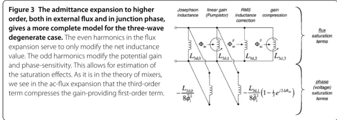
Figure 3 The admittance expansion to higher order, both in external flux and in junction phase, gives a more complete model for the three-wave degenerate case.The even harmonics in the flux expansion serve to only modify the net inductance value. The odd harmonics modify the potential gain and phase-sensitivity. This allows for estimation of the saturation effects. As it is in the theory of mixers, we see in the ac-flux expansion that the third-order term compresses the gain-providing first-order term.

that the contribution ofφ˜

 should be negligible when the following is true.

| ˜φ| √

 ()

As in the previous consideration of the nonlinearity due toac/, this is not particu-larly a remarkable constraint. The phase amplitude√ is obviously already a large fraction ofπ. It only reinforces the point that| ˜φ|should be quite small compared to this value. Perhaps, though, it is worthwhile to point out this limit also corresponds directly to a limit on the junctionvoltage, by way of the ac Josephson effect.

|V|=φ˜

ω π

√



π ω ()

Concluding discussion of saturation effects due to flux and to signal phase, we turn to Figure . Here, we combine the effects of gain compression into a common model. As in the theory of mixers, we see that the odd terms in the expansion account for both gain and its saturation.

5 The four-wave degenerate case

Next, we take interest in the SQUID with zero dc flux. When the dc flux is zero, the first derivative of inductance as a function of flux is also zero. We notice from Eq. () that

Ld, becomes infinite (an “open”) and no longer contributes to the circuit. In fact, all of the odd powers ofacwill disappear from the “flux” term of Eq. (). The reason for this can be attributed to the symmetric behavior of the unbiased device. Yet it is still possible to achieve parametric amplification among the even harmonics of the admittance expansion in flux, in a degenerate case without an idler tone distinct from a signal (ω=ω). In this case one must usefour-wave degeneratemixing, where we can consider this astwopump photons interacting with a signal photon and an idler photon (i.e.,ω+ω= ω).

The four-wave degenerate case:

ω=ω= (ω–ω) =ω ()

As in the three-wave degenerate case, both idler and signal tones occur at identically the same frequency and we consider only the disturbance of their combined response. Again, we treat this degenerate tone as thesignal(ω) response.

response, we need to expand the “flux” term of Eq. () tond-orderfor thiszero flux-bias case.

Iccos(π δ/)≈Ic–Ic

π 

 (δ)

=Ic–

Ic

(δf) _cos(ω

t+θ)



()

As in Eq. (), we find the total current at the signal frequency by multiplying our “flux” approximation by the “phase” term approximation. We use the approximation for the sig-nal phase as in Eq. (). The resulting sigsig-nal current, asig-nalogous to Eq. () but withω=ω, becomes

i(t)+=  Icφ˜

 –  (δf)



ejθ_ejωt_–  Icφ˜

∗

(δf)ej

θ–jθ_ejωt _()

Considering the small-signal voltage of Eq. (), we find the signal admittance in the four-wave degenerate case to be

Yd(ω) = Icπ

jω – Icπ

jω

(δf)– Icπ

jω

(δf)ejθ–jθ _() = (jωLd,)–+ (jωLd,a)–+ (jωLd,b)– ()

In this case, we have defined the following.

Four-wave degenerate amplifier:

Ld,=LJ

Ld,a= –LJ

 δf



Ld,b= –LJ

 δf



ejθd θd= (θ–θ)

()

So we find that the admittance which is proportionate to (δf)_{has both phase-insensitive} and phase-sensitive terms. Note also the dependence on the pump phase inθdis differ-ent by  compared to the phase angleθdof Eq. (). Also in this four-wave degenerate case, we can produce a negative resistance, and consequently gain, from theLd,bterm by adjustingθdaccordingly.

In the next sections, we turn to the more general case ofnondegenerateoperation. There, the idler response must now be considered separately from the signal response.

6 General conditions for nondegenerate parametric effects using the small-signal admittance matrix

We now consider specificallynondegeneratemixing conditions. Here, “nondegenerate” asserts its standard meaning that all frequency terms under consideration are unique,i.e., ωi=ωjfor allj=i. Where any of our six considered mixing frequencies (Table ) may

As before, the SQUID current is directly related to the junction phase by the dc Joseph-son effect as in Eq. (). However, we include a nd-order expansion of the “flux” term of Eq. (), which also includes dc flux. In this case, expanding the “flux” term to nd-order ensures nontrivial couplings to most frequency components. We wish to find the contributions of the current at different frequencies, given by the formi(t) =_n=in(t) as

in Eq. (). For a single frequency component of the junction phase, we find the current amplitudes at all considered frequencies.

Although we could present a matrix of frequency couplings by what we have just de-scribed, we wish to find anadmittance matrixrelating current and voltage amplitudes. We therefore translatejunction phaseamplitudes intovoltageamplitudes by way of the ac Josephson effect. Starting from Eq. (), we find the following.

φn(t) =

π 

vn(t)dt= –j

π ωn

Vnejωnt+j

π ωn

V_n∗e–jωnt ()

Taking into consideration how frequency components of the voltage couple to both con-jugate and non-concon-jugate terms of the current, we arrive at our desired small-signal ad-mittance matrix. Rather than a basis set of physical ports as in a multi-terminal device, here the admittance matrix “ports” (indices) represent the frequencies from Table .

⎛ ⎜ ⎜ ⎜ ⎜ ⎜ ⎜ ⎝ I

I∗

I

I_∗ I ⎞ ⎟ ⎟ ⎟ ⎟ ⎟ ⎟ ⎠ =  jLJ ⎛ ⎜ ⎜ ⎜ ⎜ ⎜ ⎜ ⎜ ⎜ ⎜ ⎝ 

ω –

∗



ω 

ω –

∗  ω  ω 

ω –



ω 

ω –

∗



ω 

∗



ω –

∗



ω 

ω 



ω 

ω –



ω  –



ω 

∗



ω 

∗



ω 

 ω ⎞ ⎟ ⎟ ⎟ ⎟ ⎟ ⎟ ⎟ ⎟ ⎟ ⎠ ⎛ ⎜ ⎜ ⎜ ⎜ ⎜ ⎜ ⎝ V

V∗

V

V_∗ V ⎞ ⎟ ⎟ ⎟ ⎟ ⎟ ⎟ ⎠ ()

We do not list in this matrix the pump current amplitude,I, as it couples to none of the other six frequencies but its own (ω).

This admittance matrix holds true as long as the pump frequency is larger than the sig-nal frequency (ω>ω) so that the “three-wave difference idler” frequency remains posi-tive (ω> ). In the case ofω<ω, some matrix elements appear instead with conjugate quantities. Similar redefinitions are also necessary if frequencyω= ω–ωwere also to become negative. We consider the conditions (ω> ) and (ω> ) to be the standard situation.

We find again the quiescent Josephson inductance, LJ = _πIccos(F). Some new, flux-dependent terms , , and  also appear, which are not indexed by frequency. Rather, their indices indicate the order of the series expansion in flux for which they first become nontrivial. Their expressions are the following.

=  –  δf

 _()

= δf

 tan(F)e

–jθ _()

= δf

 e

–jθ _()

To note, for vanishingδf =π ac

The importance of the matrix equation (Eq. ()) should be emphasized. This tells us the response of a flux-pumped SQUID between all relevant frequency components, but yet it can be used in the same form as any other n-port admittance matrix from circuit theory. So for this very general degenerate case, we may now consider a large number of three-wave and four-wave mixing devices, both as negative-resistance amplifiers and as frequency converters. It further allows us to describe a number of next-order effects which also occur in these devices.

The elements of the admittance matrix (Eq. ()), are specifically theshort-circuit ad-mittance parameters []. This is defined as the following,

Ykl=

Ik

Vl

Vm=,m=l

()

whereVm=  withm=lis a condition met by shorting all ports,mother than the port of

interest,l.

In the next section, we begin by considering a special case of Eq. () where the de-sired harmonics form a subset of the admittance matrix. The unwanted components are assumed to be zero (i.e., shorted). We will then find necessary corrections for when un-wanted harmonics are insteadopen-circuited.

7 The three-wave nondegenerate negative-resistance parametric amplifier

When the signal frequency under consideration is not degenerate relative to the pump frequency, the findings of Sections  and  break down. We now return to considerations of three-wave mixing, but for thenondegeneratecase whereω=ω/. In this case, it is necessary to provide for the presence of anidlerjunction phase (voltage) atω. The idler comes about due to the nonlinear frequency coupling between the signal and pump terms. A response at the idler frequency need not be induced at the input, nor measured as an output variable, for it to play an important role as an internal state variable.

In this section, we consider the following conditions on the signal and idler frequencies.

The three-wave nondegenerate case:

ω= (ω–ω)=ω ()

We consider the matrix subset of Eq. () corresponding to a signal atωand the idler atω. The circuit at all other harmonics is assumed to be shorted.

I

I_∗

= 

jLJ



ω –

∗



ω 

ω –



ω

V

V_∗

()

This provides the current and voltage relations directly across the SQUID at the signal and idler frequencies. Next, we generalize the circuit such that we take into account the possible effects of other generator and load admittances.

7.1 Understanding this three-wave nondegenerate model as a circuit topology

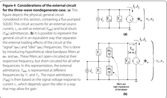
Figure 4 Considerations of the external circuit for the three-wave nondegenerate case.(a) This figure depicts the physical, general circuit

considered in this section, containing a flux-pumped SQUID. This circuit accounts for an external source current,is, as well as external (Yext) and local shunt (Ysh) admittances. (b) It is possible to represent the general circuit in an equivalent way that separates the external loading effects of the circuit at the “signal” (ω1) and “idler” (ω2) frequencies. This is done by introducing hypothetical, ideal bandpass filters at

ω1andω2. These filters act open-circuited at their respective frequency, but short-circuited for all other frequencies. In this representation, the external admittance,Yext, is represented at different frequencies byY1andY2. The input admittance (YSQ) is then based on the signal voltage response to currenti1, which depends upon the idler in a way that may allow for gain.

its amplitude isIsand its frequency isω. This external current source may be loaded by an

external admittance,Yext. The currentsi(t) andi(t), with amplitudesIandI, continue to indicate the currents directly into the SQUID at frequenciesω andω, respectively. We account for either parasitic or intentional admittances directly across the SQUID by the termYsh(ω), which may be frequency dependent. We make a distinction betweenYext andYsh(ω) since the definition of available power from the external source involves only Re[Yext].

In Figure (b), we depict how we can think of the effects of the external load at different frequencies by recasting this circuit in an equivalent representation. In this case, we sepa-rateYextinto distinct impedancesYat frequencyωandYat frequencyω. We introduce hypothetical bandpass filters which isolateYandYto their respective frequencies out-side of the pumped SQUID. These ideal filters work by providing a high-impedance (open) at their intended frequencies, while at all other frequencies they serve as a perfect short. This topology ensures that all unwanted frequencies short the SQUID, preventing any voltage at those frequencies to accumulate. Thus, we are able to reduce the general admit-tance matrix of Eq. () to the much simpler matrix of Eq. (). While we do not actively source the idler current, we will find that the external admittance at the idler frequency,

Y, effects response of the SQUID at the signal frequency in an important way.

7.2 The voltage and current ratios of the three-wave nondegenerate parametric amplifier

We are not quite ready to understand how gain appears in this system. This nondegen-erate case is complicated by the appearance of an idler response distinct from the signal. For instance, the idler-to-signal voltage ratio V∗

section. In what follows, we complete an analysis of our generalized circuit to solve for the idler voltage and current in terms of the signal.

Regarding the general circuit as depicted in Figure , we use Kirchhoff ’s node equations for both the signal and idler.

Is–VY–I=  ()

–V_∗Y_∗–I_∗=  ()

Above, we defined the grouped admittancesY_=Y+Ysh(ω) andY=Y+Ysh(ω). To go further, the coupled subsystem of Eq. () allows us to eliminateIandI∗, giving the following.

Is=V

Y_+ 

jωLJ

–V

∗

 ∗

jωLJ

()

 = V 

jωLJ

+V_∗

Y_∗– 

jωLJ

()

Equations () and () now represent the current and voltage response of the generalized circuit depicted in Figure . Since thesignal currentis sourced in this model, what remains to be solved are the voltage disturbances V andV∗. We define the impedancesZL=

jωLJ/ andZL=jωLJ/ . The voltage amplitudes are then found to be

V=LJZLωω

Y_∗ZL– 

Is

()

V_∗=jLJZLZL ω

Is

()

where the denominator term,, is proportionate to the determinant formed by the matrix of Eqs. () and ().

=L_Jωω(YZL+ )

Y_∗ZL– 

–ZLZL| | ()

When we consider thevoltage ratiobetween the idler and signal, the cumbersome de-nominator cancels, providing the more simple relation

V_∗ V

=ω  ω 



 +Z∗_LY_∗ ()

HereZ_L∗_Y_∗, we see Eq. () go to the limit

lim

Z∗LY∗→

V_∗ V

=ω  ω 

= ω ω

δf

 –_δftan(F)e

–jθ _()

On the other hand, when this quantity becomes large such thatZ_L∗_Y_∗, we see

lim

Z∗_LY_∗→∞

V_∗

V

So the voltage of the idler response is of course a function of how well the external circuit is being kept “open” at the idler frequency,ω.

We can also find the idler-to-signalcurrent ratio. For this we revisit the system repre-sented by Eq. (), and divide its second equation by its first. We substitute the signal and idler voltage amplitudes found in Eqs. () and (). This gives the following.

I_∗ I

=  



 + 

Z_L∗_Y_∗+

||  

ω

ωZLY∗

()

We can look at the admittance limits of the current ratio as well. When the external ad-mittance is small, we see

lim

Z∗_LY_∗→

I_∗ I

=  ()

Conversely, when external admittance is large, we see

lim

Z∗_LY_∗→∞

I_∗ I

=  

= 

δf

 – δf

tan(F)e–jθ _()

These limits are intuitive. We can see the idler current will be inhibited when the external circuit is comparatively more “open,” representing a small external admittance. Note the similar behavior indicated between Eqs. () and (), as well as between Eqs. () and ().

These quantities depict the response of the circuit at the idler frequency,ω, relative to the circuit behavior at the signal frequency,ω. We will now utilize this understanding in the next section to find how this system acts as a negative-resistance amplifier.

7.3 The input impedance of the nondegenerate three-wave parametric amplifier

To understand how this system works as an amplifier, we must find how it provides a neg-ative resistance at the signal frequency. To this end, we seek to find the input admittance as seen atω.

The input admittance as seen into the device at the signal frequency we can say isYSQ=

IV, giving

YSQ=

I

V = 

ZL –V

∗



V

∗

 



ZL

()

Recall that ≈ to first order. To interpret Eq. () as animpedance, this is the Josephson inductance again in parallel to some other term. To find this other term, which is repre-sented (as an admittance) by the second term on the right-hand side of Eq. (), we must incorporate the ratio V∗

V from Eq. (). Substituting this term into Eq. (), we arrive at

YSQ= 

ZL –| |

  



ZL 

 +Z∗_LY_∗ ()

= (jωLn,)–+ (jωLn,)– ()

Figure 5 This figure depicts the equivalent signal impedance of the flux-pumped SQUID in the three-wavenondegeneratecase.The constituent inductances are given by Eq. (66). In the limit that the ac-flux is small such thatγ0≈1, the inductanceLn,0is simply the quiescent Josephson inductance and Ln,2∝2ac. TheLn,2acquires an imaginary component due to the external (real) admittance at the idler frequency. A positive, imaginaryinductanceis anegative,real impedance, which may therefore provide gain.

on thepump phase is no longer present. Thisnondegenerateamplifier, therefore, isphase insensitive. The following terms for inductances are used.

Three-wave nondegenerate amplifier:

Ln,=LJ/ε

Ln,= –

LJ

|ε|

ε–jωLJY∗

()

Above, the “Ln,” inductance is once again simply the Josephson inductance in the small-signal limit. The “Ln,” inductance, in parallel toLn,, contains two terms which are both proportionate to| |–. The first term is negative and simply modifies the net inductance by a small correction, making the net inductance appear bigger as the ac flux increases. The second term ofLn,depends onY∗in an important way, providing the possibility for gain in this scenario. IfY_∗has a real and positive component, this allows the impedance represented byLn, to acquire anegativeand real component. Therefore theY∗term of

Ln,acts as an active impedance converter, allowing the impedance external to the SQUID at the idler frequency to appear, transformed, at the signal frequency. We may think of the input admittance (or input impedanceZSQ= /YSQ) directly into the three-wave nonde-generate pumped SQUID as depicted in Figure .

We comment on thefrequency dependenceofLn,. If we subscribe to axiomatic circuit theory [–], our linearized inductances should have a dependence strictly proportional tojω. The second term inLn,, which is the same term that may act as a negative resistance, also contains an extra factor,jω=j(ω–ω). This gives a maximum of the productωω atω/, which for this reason is whyω/ is the frequency of maximum parametric am-plification (or nearly so) in a three-wave nondegenerate amplifier. Between an uncommon frequency dependence and negative-resistance behavior, it may be logical to consider this second term ofLn,as relating to something other than an inductance. Yet we choose keep the terminology of an inductance only for consistency.

7.4 The three-wave nondegenerate amplifier: transducer gain

The common readout implementation for a parametric amplifier (e.g., a flux-pumped SQUID) is as a reflection device coupled to a circulator and a nd-stage amplifier (e.g., a high electron mobility transistor (HEMT)) [, , , –]. It is therefore important that the first-stage gain of a parametrically flux-pumped SQUID be adequate to overcome the noise of subsequent gain stages. An insightful quantity in this context (in addition, say, to other quantities such as anoise figure) is thetransducer gainof the device. It is straight-forward to specify the transducer gain, considering the simplified circuit we have so far described in this section.

The transducer gain is the ratio of the output power to the available input power. We consider the source admittance as Y. For the(rms) available input powerat the signal frequency, we find

Pa,=

I

s

Re[Y] ()

We consider the output signal to be reflected back onto the input admittance, such that we say the(rms) output poweris

Po,=

V_

 Re[Y] ()

The transducer gain is then

GT=

Po,

Pa, =V



(Re[Y])

I

s

=  (Re[Y])  |Y_+YSQ|

()

This can be expressed as

GT=

Re[Y] (_ω 

Ln,+

Re[Ln,]

ω|Ln,| –Im[Y

])+ (

Im[Ln,]

ω|Ln,| –Re[Y

])

()

whereLn,andLn,are from Eq. ().

7.5 Adding open-circuited terms

As anadmittance model, as opposed to an impedancemodel, the ideal case is for all non-intentional harmonics to be subject to an infinite admittance external to the pumped SQUID (e.g., to have a shorted external load at frequencies other than the signal and idler). This prevents voltages at these other frequencies from accumulating across the SQUID, thereby removing their influence from the admittance matrix and the resulting mixed cur-rents. Conversely, when the external impedance is nontrivial at other frequencies, other harmonics will modify the description we have just presented.

Figure 6 This figure demonstrates the parametric interaction of theopen-circuitedSQUID at the signal and idler frequencies.As opposed to Section 7.1, theseseriesbandpass filters are nowzero

impedance at bandpass and blocking at all other frequencies. This works in such a way that frequencies other thanω1andω2now present an open circuit to the pumped SQUID. Therefore the voltage across the SQUID is not necessarily zero at these other frequencies. These additional mixing effects can be mapped onto a modifiedsubsystem between signal and idler, which is the 2×2 matrix of Eq. (71).

and idler (ω) frequencies. To reach a manageable solution, we assume the limiting condi-tions ≈ and ≈ for currents atω,ω, andω. If we keep terms up toδf, we find the signal-idler subset matrix has the simple form,

I

I_∗

= 

jLJ

⎛ ⎝εω[ –

|ε|

ε ] –

ε∗_ ω

ε

ω –

ε

ω[ –

|ε|

ε ]

⎞ ⎠

V

V_∗

()

We find this system identical to that of Eq. (), except for the multiplicative correction factor in square brackets, [ – |ε|

ε ], appearing in the two matrix elements of the main diagonal. This correction factor may become significant even for reasonably smallδf as the dc flux,F, approachesπ/. This is the notable difference between this open-circuited case and the short-circuited case we treated in Section ..

We illustrate the open-circuited case as an equivalent circuit in Figure . We depict signal and idler circuits now directly in parallel to the pumped SQUID. As opposed to the short-circuited case depicted in Figure (b), here the ideal filters are accomplishedin series

such that only the permitted frequency is allowed to pass, while all other frequencies see an open-circuit.

In this section, we have determined the response of the three-wavenondegenerate am-plifier as an impedance model. This is analogous to the “pumpistor” models we found for the three-wave and four-wave degenerate cases treated in Sections  and . A notable dif-ference in this nondegenerate case is that the external admittance at the idler frequency now determines the negative resistance. As can be seen by Eq. (), for a negative re-sistance to occur at the signal frequency, it is necessary that the circuit external to the SQUID at the idler frequency appear as a positive and real admittance. By treating both a “short-circuited” and an “open-circuited” model, we found that a finite external admit-tance at harmonics other than the signal and idler frequencies may also affect amplifier performance.

8 Conclusions

general classes of parametric driving, a flux-pumped SQUID can be described at the sig-nal frequency as a Josephson inductance in parallel to an effective, flux-dependent circuit element, “the pumpistor.” Parametric amplification can be intuitively understood within this framework, as the pumpistor impedance manifests in whole or in part as a negative resistance.

We reviewed three-wave degenerate pumping, which explains why gain in this case should bephase sensitivebetween the signal and pump. For this case, we also extended our impedance approximation to demonstrate how the SQUID saturates both by pump flux and by junction phase (or voltage). We also depicted the four-wave degenerate case which is appropriate when the device is biased with zero-flux. Here, the pumpistor ele-ment is inversely proportionate to thesquareof the ac flux. We found this case also to be phase sensitive, but with a slightly different signal-to-pump difference than in the three-wave degenerate case.

We also depicted nondegenerate pumping in a very general sense, using a matrix equa-tion formalism. This formalism accounts for the presence of one or up to four “idler” fre-quencies which occur as mixing tones between the pump and the signal response. Many three- and four-wave nondegenerate parametric phenomena can be interpreted from this matrix, including effects such as frequency up- and down-conversion. Using a subset of these matrix equations, we treated the three-wave nondegenerate amplifier, where the signal and single idler are considered. By solving for an idler distinct from the signal, we found that the pumpistor impedance was nowphase insensitive. We found the negative resistance responsible for gain was now dependent on the external circuit admittance at the idler frequency. With regards to the other, higher harmonics, we treated the three-wave nondegenerate amplifier in both the “short-circuited” and “open-circuited” approxi-mations. While all of these models operate under a classical, circuit-theoretic framework rather than a quantum optics framework, they should be of great benefit for future designs of experiments using superconducting circuits for quantum information purposes.

Competing interests

The authors declare that they have no competing interests.

Authors’ contributions

KMS derived most of the equations. Both authors developed the concept and wrote this paper together.

Author details

1_{Electrical and Computer Engineering, Texas A&M University, College Station, TX 77843, USA.}2_{Microtechnology and}

Nanoscience, Chalmers University of Technology, Göteborg, SE-412 96, Sweden.

Acknowledgements

We acknowledge support from the EU through the ERC and the projects SOLID, SCALEQIT, and PROMISCE, as well as from the Swedish Research Council and the Wallenberg Foundation. We are also grateful for fruitful discussions with Chris Wilson, Seckin Kinta¸s, Michaël Simoen, Philip Krantz, Martin Sandberg, and Jonas Bylander.

Received: 31 October 2013 Accepted: 6 January 2014 Published: 7 March 2014

References

1. Caves CM:Quantum limits on noise in linear amplifiers.Phys Rev D1982,26(8):1817-1839.

2. Feldman MJ, Parrish PT, Chiao RY:Parametric amplification by unbiased Josephson junctions.J Appl Phys1975, 46(9):4031-4042.

3. Taur Y, Richards PL:Parametric amplification and oscillation at 36 GHz using a point-contact Josephson junction. J Appl Phys1977,48(3):1321-1326.

4. Feldman MJ:The thermally saturated SUPARAMP.J Appl Phys1977,48(3):1301-1310.

5. Wahlsten S, Rudner S, Claeson T:Parametric amplification in arrays of Josephson junctions.Appl Phys Lett1978, 30:298-300.

7. Yurke B, Kaminsky P, Miller R, Whittaker E, Smith A, Silver A, Simon R:Observation of 4.2-K equilibrium-noise squeezing via a Josephson-parametric amplifier.Phys Rev Lett1988,60(9):764.

8. Yurke B, Corruccini LR, Kaminsky PG, Rupp LW, Smith AD, Silver AH, Simon RW, Whittaker EA:Observation of parametric amplification and deamplification in a Josephson parametric amplifier.Phys Rev A1989, 39(5):2519-2533.

9. Castellanos-Beltran M, Lehnert KW:Widely tunable parametric amplifier based on a superconducting quantum interference device array resonator.Appl Phys Lett2007,91:083509.

10. Eichler C, Bozyigit D, Lang C, Baur M, Steffen L, Fink JM, Filipp S, Wallraff A:Observation of two-mode squeezing in the microwave frequency domain.Phys Rev Lett2011,107(11):113601.

11. Hatridge M, Vijay R, Slichter DH, Clarke J, Siddiqi I:Dispersive magnetometry with a quantum-limited squid parametric amplifier.Phys Rev B2011,83(13):134501.

12. Yamamoto T, Inomata K, Watanabe M, Matsuba K, Miyazaki T, Oliver WD, Nakamura Y, Tsai JS:Flux-driven Josephson parametric amplifier.Appl Phys Lett2008,93(4):042510.

13. Wilson CM, Duty T, Delsing P:Parametric oscillators based on superconducting circuits. In:Fluctuating Nonlinear Oscillators. Edited by Dykman M. Oxford: Oxford University Press; 2012.

14. Sundqvist KM, Kintas S, Simoen M, Krantz P, Sandberg M, Wilson CM, Delsing P:The pumpistor: a linearized model of a flux-pumped superconducting quantum interference device for use as a negative-resistance parametric amplifier.Appl Phys Lett2013,103(10):102603.

15. Tholen EA, Ergul A, Doherty EM, Weber FM, Gregis F, Haviland DB:Nonlinearities and parametric amplification in superconducting coplanar waveguide resonators.Appl Phys Lett2007,90:253509.

16. Ho Eom B, Day PK, LeDuc HG, Zmuidzinas J:A wideband, low-noise superconducting amplifier with high dynamic range.Nat Phys2012,8(8):623-627.

17. Mallet F, Ong FR, Palacios-Laloy A, Nguyen F, Bertet P, Vion D, Esteve D:Single-shot qubit readout in circuit quantum electrodynamics.Nat Phys2009,5(11):791-795.

18. Vijay R, Macklin C, Slichter DH, Weber SJ, Murch KW, Naik R, Korotkov AN, Siddiqi I:Stabilizing rabi oscillations in a superconducting qubit using quantum feedback.Nature2012,490:77-80.

19. Flurin E, Roch N, Mallet F, Devoret MH, Huard B:Generating entangled microwave radiation over two transmission lines.Phys Rev Lett2012,109(18):183901.

20. Steffen L, Salathe Y, Oppliger M, Kurpiers P, Baur M, Lang C, Eichler C, Puebla-Hellmann G, Fedorov A, Wallraff A: Deterministic quantum teleportation with feed-forward in a solid state system.Nature2013,500:319-322. 21. Abdo B, Schackert F, Hatridge M, Rigetti C, Devoret MH:Josephson amplifier for qubit readout.Appl Phys Lett2011,

99(16):162506.

22. Blackwell LA, Kotzebue KL:Semiconductor-Diode Parametric Amplifiers. Englewood Cliffs: Prentice Hall; 1961. 23. Decroly JC:Parametric Amplifiers. New York: Wiley; 1973.

24. Howson DP, Smith RB:Parametric Amplifiers. London: McGraw-Hill; 1970.

25. Josephson BD:Possible new effects in superconductive tunnelling.Phys Lett1962,1:251-253.

26. Zagoskin AM:Quantum Engineering: Theory and Design of Quantum Coherent Structures. Cambridge: Cambridge University Press; 2011.

27. Van Duzer T, Turner CW:Principles of Superconductive Devices and Circuits. 2nd edition. Upper Saddle River: Prentice Hall; 1999.

28. Tinkham M:Introduction to Superconductivity. 2nd edition. New York: McGraw-Hill; 1996. 29. Maas SA:Microwave Mixers. Dedham: Artech House; 1986. [The Artech House Microwave Library.] 30. Chen W-K:Active Network and Feedback Amplifier Theory. New York: McGraw-Hill; 1980. 31. Chua LO:Introduction to Nonlinear Network Theory. New York: McGraw-Hill; 1969.

32. Chua LO, Desoer CA, Kuh ES:Linear and Non-linear Circuits. New York: McGraw-Hill; 1987. [McGraw-Hill Series in Electrical and Computer Engineering.]

33. Chua LO:Nonlinear circuit foundations for nanodevices.Proc IEEE2003,91(11):1830-1859.

doi:10.1140/epjqt6

Cite this article as:Sundqvist and Delsing:Negative-resistance models for parametrically flux-pumped