A chronicle of galaxy mass assembly in the EAGLE simulation

Advance Access publication 2016 September 27

A chronicle of galaxy mass assembly in the EAGLE simulation

Yan Qu,

John C. Helly,

Richard G. Bower,

Tom Theuns,

Robert A. Crain,

Carlos S. Frenk,

Michelle Furlong,

Stuart McAlpine,

Matthieu Schaller,

Joop Schaye

and Simon D. M. White

1_{National Astronomical Observatories, Chinese Academy of Sciences, 20A Datun Road, Chaoyang, Beijing 10012, China} 2_{Institute of Computational Cosmology, Durham University, South Road, Durham DH1 3LE, UK}

3_{Astrophysics Research Institute, Liverpool John Moores University, 146 Brownlow Hill, Liverpool L3 5RF, UK} 4_{Leiden Observatory, Leiden University, Postbus 9513, NL-2300 RA Leiden, the Netherlands}

5_{Max-Planck-Institut f¨ur Astrophysik, Karl-Schwarzschild-Strae 1, D-85741 Garching, Germany}

Accepted 2016 September 26. Received 2016 August 29; in original form 2016 March 28

A B S T R A C T

We analyse the mass assembly of central galaxies in the Evolution and Assembly of Galaxies and their Environments (EAGLE) hydrodynamical simulations. We build merger trees to connect galaxies to their progenitors at different redshifts and characterize their assembly histories by focusing on the time when half of the galaxy stellar mass was assembled into the main progenitor. We show that galaxies with stellar massM_∗<1010.5_{Massemble most of}

their stellar mass through star formation in the main progenitor (‘in situ’ star formation). This can be understood as a consequence of the steep rise in star formation efficiency with halo mass for these galaxies. For more massive galaxies, however, an increasing fraction of their stellar mass is formed outside the main progenitor and subsequently accreted. Consequently, while for low-mass galaxies, the assembly time is close to the stellar formation time, the stars in high-mass galaxies typically formed long before half of the present-day stellar mass was assembled into a single object, giving rise to the observed antihierarchical downsizing trend. In a typical present-dayM_∗ ≥1011_M

galaxy, around 20 per cent of the stellar mass has an external origin. This fraction decreases with increasing redshift. Bearing in mind that mergers only make an important contribution to the stellar mass growth of massive galaxies, we find that the dominant contribution comes from mergers with galaxies of mass greater than one-tenth of the main progenitor’s mass. The galaxy merger fraction derived from our simulations agrees with recent observational estimates.

Key words: galaxies: evolution – galaxies: formation – galaxies: high-redshift – galaxies: interactions – galaxies: stellar content.

1 I N T R O D U C T I O N

In the cold dark matter (CDM) cosmological model, the growth of dark matter haloes is largely self-similar, with larger haloes be-ing formed more recently than their low-mass counterparts. The formation and assembly of galaxies are, however, much more com-plex. Feedback from massive stars and the formation of black holes generates a strongly non-linear relationship between the masses of dark matter haloes and those of the galaxies they host. For low-mass haloes (with mass1011.5_M

), the stellar mass increases rapidly, with a slope of∼2, but in higher mass haloes, the stellar mass of the main (or ‘central’) galaxy increases much more slowly than the

_{E-mail:[email protected]}

halo mass, with a slope of∼0.5 (e.g. Benson et al.2003; Behroozi, Wechsler & Conroy2013; Moster, Naab & White2013). The mass assembly of galaxies will therefore be quite different from those of their parent haloes. Establishing how galaxies assemble their stars over cosmic time is then central to understanding galaxy formation and evolution.

One question we need to answer is the relative importance of the growth of galaxies via internal ongoing star formation (‘in situ’), in comparison to the mass contributions of external processes (e.g. Guo & White2008; Zolotov et al.2009; Oser et al.2010; Font et al.

mass (‘accretion’). While major mergers can rapidly increase a galaxy’s stellar mass, minor mergers are much more common (e.g. Hopkins et al.2008; Parry, Eke & Frenk2009).

To evaluate the relative importance of mergers to galaxy assem-bly, we need to know their merging histories. From an observational perspective, counts of close galaxy pairs (e.g. Williams, Quadri & Franx2011; Man, Zirm & Toft2014), or galaxies with disturbed morphologies (e.g. Lotz et al.2008; Conselice, Yang & Bluck2009; L´opez-Sanjuan et al.2011; Stott et al.2013), provide a census of galaxy mergers. These values can be further converted into galaxy merger rates through the use of a merger time-scale (e.g. Kitzbichler & White2008). Unfortunately, those methods have their own lim-itations: galaxies in close-pairs may not be physically related, and may be chance line-of-sight superpositions; morphological distur-bances are not unique to galaxy mergers. For example, clumpy star formation driven by gravitational instability can also foster the for-mation of galaxies with irregular morphologies (Lotz et al.2008). In addition, these methods are sensitive to the merger stage and the mass ratio of the merging galaxies. Due to these limitations, the scatter between merger rate measurements is large, and it is difficult to make a reliable assessment of the complementary contribution of mergers to galaxy growth. Recently, deep surveys have begun to shed more light on the galaxy merger rate at high redshifts (e.g. Man et al.2014). Even so, the evolution of the merger rate remains controversial. An alternative approach is to extract the merger rates of galaxies from a model that reproduces the observed abundance of galaxies (and their distribution in mass), and its evolution with redshift, in a full cosmological context.

In the hierarchical structure formation scenario, the assembly of galaxies is believed to be closely related to the formation histories of their parent haloes. The practice of using halo merger histories to understand the build-up of galaxies can be traced back to Bower (1991), Cole (1991), and Kauffmann, White & Guiderdoni (1993). In these pioneering works, the growth of haloes is described by analytical methods. Numerical techniques likeN-body numerical simulations can deal more accurately with the gravitational pro-cesses underlying the evolution of cosmic structure. The clustering of haloes is tracked, snapshot by snapshot, and stored in a tree form (‘merger tree’). Halo merger trees therefore record, in a direct way, when and how haloes assemble by accreting other building blocks, and are widely used to rebuild galaxy assembly histories (e.g. Kauffmann et al.1993,1999; Roukema et al.1997; Springel et al.2001).

To compute galaxy merger rates, one possibility is to combine the halo merger trees with a redshift-dependent abundance match-ing model that statistically assigns galaxies to dark matter haloes (Fakhouri & Ma2008; Behroozi et al.2013; Moster et al.2013). In this fashion, the observed abundance of galaxies can be inverted to estimate the galaxy merger rate as a function of halo mass and redshift. This provides a great deal of insight, but relies on the accuracy of the statistical model. Although appealing because of its close relation to the real data, the approach may miss physical correlations between the merging objects. A preferable approach is therefore to form galaxies within dark matter haloes using a physical galaxy formation model. It is important to note, however, that reli-able conclusions can only be obtained if the overall galaxy stellar mass function accurately reproduces observational measurements (Benson et al.2003; Schaye et al.2015).

One approach is to use ‘semi-analytic’ models of galaxy forma-tion. By introducing phenomenological descriptions for feedback from star formation and active galactic nuclei (AGN), such mod-els are able to reproduce the observed galaxy stellar mass function

(e.g. Bower et al.2006; Croton et al.2006, for a recent review, see Knebe et al.2015). De Lucia et al. (2006) study the assembly of elliptical galaxies in a semi-analytic model based on the model of Croton et al. (2006). They find that stars in massive galaxies (with stellar massM_∗≥1011_M

) are formed earlier (z2.5) but are as-sembled later (byz≈0.8). De Lucia & Blaizot (2007) show further that massive members in galaxy clusters assemble through mergers late in the history of the Universe, with half of their present-day mass being in place in their main progenitor byz≈0.5. In contrast, less massive galaxies undergo relatively few mergers, acquiring only 20 per cent of their final stellar mass from external objects. Parry et al. (2009) study the assembly and morphology of galaxies in the semi-analytic model of Bower et al. (2006). They found many similarities, but also important disagreements, stemming primarily from the differing importance of disc instabilities in the two mod-els. Parry et al. (2009) find that major mergers are not the primary mass contributors to most spheroids except the brightest ellipticals. This, instead, is brought in by minor mergers and disc instabilities. In their model, the majority of ellipticals, and the overwhelming majority of spirals, never experience a major merger.

Semi-analytic studies such as those above give important insights but suffer from the limitations inherent to the approach, for example, the neglect of tidal stripping of infalling satellites and the absence of information about the spatial distribution of stars, as well as being limited by the overall accuracy of the model. Numerical simulations have fewer limitations, and have thus become an alternative useful tool for these studies. Hopkins et al. (2010) compare the galaxy merger rates derived from a variety of analytical models and hydro-dynamical simulations. They find that the predicted galaxy merger rates depend strongly on the prescriptions for baryonic physical pro-cesses, especially those in satellite galaxies. For example, the lack of strong feedback can result in a difference in predicted merger rates by as much as a factor of 5. Mass ratios used in merger clas-sification also have an impact on merger rate prediction. Using the stellar mass ratio, rather than the halo mass ratio, can result in an order of magnitude change in the derived merger rate.

With rapidly increasing computational power and much pro-gresses in modelling physical processes on subgrid scales, cosmo-logicalN-body hydrodynamical simulations are increasingly capa-ble of capturing the physics of galaxy formation (e.g. Hopkins et al.

galaxies, avoiding the complications of environmental processes such as ram pressure stripping and strangulation that suppress star formation and strip stellar mass from satellites. Unless otherwise stated, stellar masses refer to the stellar mass of a galaxy at the redshift of observation, not to the initial mass of stars formed.

The outline of this paper is as follows. In Section 2, we provide a brief overview of the numerical techniques and subgrid physi-cal models employed by the EAGLE simulations, and describe the methodology used to construct merger trees from simulation out-puts. We investigate the assembly histories and merger histories of galaxies and discuss the impact of feedback on galaxy mass build-up in Section 3. We compare our results with some previous works in Section 4, and finally summarize in Section 5. The appendices present the detailed criteria we use to define galaxy mergers and show the impacts of our choices of galaxy mass on our results. The cosmological parameters used in this work is from thePlanck mis-sion (Planck Collaboration XVI2014),=0.693,m=0.307,

h=0.677,ns=0.96, andσ8=0.829.

2 E AG L E S I M U L AT I O N A N D M E R G E R T R E E

2.1 EAGLE simulation

The galaxy samples for this study are selected from the EAGLE simulation suite (Crain et al. 2015; Schaye et al. 2015). The EAGLE simulations follow the evolution (and, where appropri-ate, the formation) of dark matter, gas, stars, and black holes from redshiftz=127 to the present day at z=0. They were carried out with a modified version of theGADGET3 code (Springel2005) using a pressure–entropy-based formulation of smoothed particle hydrodynamics method (Hopkins2013), coupled to several other improvements to the hydrodynamic calculation (Dalla Vecchia., in preparation; Schaye et al.2015; Schaller et al.2015b). The simula-tions include subgrid descripsimula-tions for radiative cooling (Wiersma, Schaye & Smith2009), star formation (Schaye & Dalla Vecchia

2008), multi-element metal enrichment (Wiersma et al.2009), black hole formation (Rosas-Guevara et al.2015; Springel, Di Matteo & Hernquist2005), as well as feedback from massive stars (Dalla Vecchia & Schaye2012) and AGN (for a complete description, see Schaye et al.2015). The subgrid models are calibrated using a well-defined set of local observational constraints on the present-day galaxy stellar mass function and galaxy sizes (Crain et al.2015).

Each simulation outputs 29 snapshots to store particle properties over the redshift range of 0≤z≤20. The corresponding time inter-val between snapshot outputs ranges from∼0.3 to∼1.35 Gyr. The largest EAGLE simulation, hereafter referred to as Ref-L100N1504, employs 15043_{dark matter particles and an initially equal number} of gas particles in a periodic cube with side-length 100 comoving Mpc (cMpc) on each side. This setup results in a particle mass of 9.7×106_M

and 1.81×106_M

(initial mass) for dark matter and gas particles, respectively. The gravitational force between particles is calculated using a Plummer potential with a softening length set to the smaller of 2.66 comoving kpc (ckpc) and 0.7 physical kpc (pkpc).

The formation of galaxies involves physical processes operating on a huge range of scales, from the gravitational forces that drive the formation of large-scale structure on 10–100 Mpc scales, to the pro-cesses that lead to the formation of individual stars and black holes on 0.1 pc and smaller scales. Such a dynamic range, 109_{in length} and perhaps 1027_{in mass, cannot be computed efficiently without} the use of subgrid models. Such models are inevitably approximate and uncertain. In EAGLE, we require that the subgrid models are

physically plausible, numerically stable, and as simple as possible. The uncertainty in these models introduces parameters whose val-ues must be calibrated by comparison to observational data (Vernon, Goldstein & Bower2010). We explicitly recognize that these mod-els are approximate and adopt the clear methodology for selecting parameters and validating the model that is described in detail in Schaye et al. (2015) and Crain et al. (2015). The subgrid parame-ters calibrated by requiring that the model fits three key properties of local galaxies well: the galaxy stellar mass function, the galaxy size – mass relation and the normalization of the black hole mass – galaxy mass relation and that variations of the parameters alter the simulation outcome in predictable ways (Crain et al.2015). We find that these data sets can be described well with physically plausible values for the subgrid parameters. We then compare the simulation with further observational data to validate the simulation. We find that it describes many aspects of the observed universe well (i.e. within the plausible observational uncertainties), including the evo-lution of the galaxy stellar mass function and star formation rates (Furlong et al.2015b), evolution of galaxy colours and luminosity functions (Trayford et al.2015). It also provides a good match to observed OVIcolumn densities (Rahmati et al.2016) and molecu-lar content of galaxies (Lagos et al.2015), as well as a reasonable description of the X-ray luminosities of AGN (Rosas-Guevara et al.

2015). The good agreement with these diverse data sets, especially those distantly related to the calibration data, provides good rea-son to believe that the simulation provides a good description of the evolution of galaxies in the observed Universe. It can therefore be used to explore galaxy assembly histories in ways that are not accessible to observational studies.

2.2 Halo identification and subhalo merger tree

Building subhalo merger trees from cosmological simulations in-volves two steps: first, we identify haloes and subhaloes as gravi-tationally self-bound structures; secondly, we identify the descen-dants of each subhalo across snapshot outputs and establish the descendant–progenitor relationship over time.

2.2.1 Halo identification

Dark matter structures in the EAGLE simulations are initially iden-tified using the ‘Friends-of-Friends’ (FoF) algorithm with a linking length of 0.2 times the mean inter-particle spacing (Davis et al.

2.2.2 Subhalo merger tree

Although they orbit within an FoF group, subhaloes survive as distinct objects for an extended period of time. We therefore use subhaloes as the base units of our merger trees: FoF group merger trees can be rebuilt from subhalo merger trees if required. The first and main step in building the merger tree is to link subhaloes across snapshots. As in Springel et al. (2005), we search the descendant of a subhalo by tracing the most bound particles of the subhalo. We use the D-Trees algorithm (Jiang et al.2014) to locate the where-abouts of theNlink=min(Nlinkmax, max(ftraceN,Nlinkmin)) most bound particles of the subhalo, whereNis the total particle number in the subhalo. We use parametersNlinkmin=10,Nlinkmax=100,ftrace=0.1 in the descendant search. The advantages of focusing on theNlink most bound particles are two-fold. On the one hand, D-Trees can identify a descendant even if most particles are stripped away leav-ing only a dense core. On the other hand, the criterion minimises misprediction of mergers during flyby encounters (Fakhouri & Ma

2008; Genel et al.2009).

The descendant identification proceeds as follows. For a subhalo

Aat a given snapshot, any subhalo at the subsequent snapshot that receives at least one particle from Ais labelled as a descendant candidate. From those candidates, we pick the one that receives the largest fraction ofA’sNlinkmost bound particles (denoted asB) as the descendant ofA.Ais the progenitor ofB. IfBreceives a larger fraction of its ownNlinkmost bound particles fromAthan from any other subhalo at previous snapshot,A is the principal progenitor ofB. A descendant can have more than one progenitor, but only one principal progenitor. The principal progenitor can be thought of as ‘surviving’ the merger while the other progenitors lose their individual identity.

Subhaloes sometimes exhibit unstable behaviour during merg-ers, complicating the descendant/progenitor search. When a sub-halo passes through the dense core of another subsub-halo, it may not be identifiable as a separate object at the next snapshot, but will then reappear in a later snapshot. From a single snapshot, there is no way to know whether the subhalo has merged with another subhalo, or has just disappeared temporarily, and we need to search a few snapshots ahead in order to know which case it falls into. In practice, we search up toNstep=5 consecutive snapshots ahead for the missing descendants. This gives us between one andNstep descendant candidates. If the subhalo is the principal progenitor of one or more candidates, the earliest candidate that does not have a principal progenitor is chosen to be the descendant. If there is no such candidate, then the earliest one will be chosen. If the subhalo is not the principal progenitor of any candidates, it will be considered to have merged with another subhalo and no longer appears as an identifiable object.

Occasionally, two subhaloes enter into a competition for bound particles. This occurs as the participants orbit each other prior to merging. In SUBFIND, the influence of a subhalo is based on its gravitational potential well. When two subhaloes are close to each other, their volumes of influence become intertwined and the def-inition of the main halo may become unclear. For example, when a satellite subhalo orbits closely to its primary host, the satellite can be tidally compressed at some stage and become denser than the host. At this point, the satellite may be classified as the central object of the halo so that most of the halo particles are assigned to it. At a later time, the original central, however, can surpass the satellite in density and reclaim the halo particles. This contest can last for several successive snapshots, accompanied by a see-saw exchange of their physical properties during the merging. Fig.1

Figure 1. A section of a subhalo merger tree illustrating how subhaloes following branches A and B exchange particles before merging. The colour of the solid symbol reflects the halo mass, while the size of the circle represents the ‘branch mass’, which is the sum of the total mass of all the progenitors sitting on the same branch. A see-saw behaviour is clearly seen in the evolution of the halo mass, which may confuse identification of the most important branch. Instead, we use branch mass to locate the main branch of the tree. In this plot, branch A has the largest branch mass and is therefore chosen as the main branch, even though its progenitors are not always the most massive ones.

shows an example in which merging haloes take turns to be classi-fied as the central host during the merging process. Overall, fewer than 5 per cent of subhalo mergers in the EAGLE simulations ex-hibit this behaviour, compatible with the statistics found by Wetzel, Cohn & White (2009). The fact that a fierce contest between sub-haloes is sometimes seen during the merging process highlights the inherent difficulties in appropriately describing subhalo properties at that stage.

The property exchanges during such periods are not physical, but rather stem from the requirement that particles be assigned to a unique subhalo on the basis of the spatial coordinates and the local density field in a single snapshot. The history of an object is, however, conveniently simplified by modifying the definition of the most massive progenitor to account for its mass in earlier snapshots. We refer to this progenitor as the ‘main progenitor’, and the branch they stay on in the object’s merger tree as the ‘main branch’. Because of the mass exchange discussed above, we track the main branch using the ‘branch mass’, the sum of the mass over all particle species of all progenitors on the same branch (De Lucia & Blaizot2007). The main progenitor is then the progenitor that has the maximum branch mass among its contemporaries. This can avoid the misidentification of main progenitors due to the property exchanges occurring for merging subhaloes as we see in Fig.1. It is worth noting that according to this definition, a lower mass progenitor which has existed for a long time can sometimes be preferred over a more massive progenitor which has formed quickly, when locating main progenitors.

The subhalo merger trees derived by the method described above are publicly available through anSQLdata base1similar to that used for the Millennium simulations (see McAlpine et al.2016, for more details).

2.3 Galaxy sample, galaxy merger tree, and merger type

In this work, galaxies are identified as the stellar components of the subhaloes. The main subhalo of a FoF halo hosts the ‘central’ galaxy, while other subhaloes within the group host satellite galax-ies. We will focus on the central galaxies in our study, avoiding the complications of environmental processes such as ram pressure stripping and strangulation that suppress star formation and strip stellar mass from satellite galaxies (e.g. Wetzel et al.2013; McGee, Bower & Balogh2014; Barber et al.2016).

The stellar mass of a galaxy is measured using a spherical aper-ture. This gives similar results to the commonly used 2D Petrosian aperture used in observational work, but provides an orientation-independent mass measurement for each galaxy. Previous studies based on the EAGLE simulations adopt an aperture of 30 pkpc to measure galaxy stellar mass (e.g. Furlong et al.2015b; Schaye et al.

2015). Nevertheless, subhaloes do contain a significant population of diffuse stars, particularly in more massive haloes (Furlong et al.

2015b). Such stars are probably deposited by interactions and tidal stripping, and sometimes observed as low-surface brightness intr-acluster/intragroup light (Theuns & Warren1997; Zibetti & White

2004; McGee & Balogh2010). Since the formation of massive galaxies is a particular focus of this paper, we use a larger aperture, with a radius of 100 pkpc, to calculate galaxy mass. Note that this mass does not include the stellar mass of satellites lying within the 100 pkpc aperture. As we will show in Appendix C, this aperture choice has little impact on galaxy properties for galaxies with stellar massM_∗<1011_M

(see also Schaye et al.2015).

Unless otherwise stated, the galaxy stellar mass in this work refers to the actual mass of stars in the galaxy at the epoch of ‘observa-tion’. Using actual mass replicates what an ideal observer would measure and directly addresses the question of when the current stellar population of the galaxy was formed/assembled. Neverthe-less, we should note that the mass budget of the current stellar population is a combination of two processes: stellar mass gain via star formation, accretion and merging, and mass-loss through stellar evolution processes. However, using the actual stellar mass complicates interpretation of the relative mass contribution from different types of merger events since it depends on the age of the stellar population that is accreted. We therefore use the stellar mass initially formed (‘initial mass’), not the actual stellar mass, to evalu-ate the contributions from internal and external processes to galaxy assembly. In practice, this distinction has little effect on the results and we show the effect of using initial stellar mass throughout in Appendix B.

2.3.1 Galaxy sample

Our study is based on the formation histories of 62 543 galax-ies in the largest EAGLE simulation Ref-L100N1504, spanning a stellar mass range of 109.5_–1012_M

over redshiftz=0–3. In order to test the robustness of our results to resolution, we also extract 1381 galaxies within the same mass range, as a com-parison sample, from the EAGLE simulation Recal-L025N0752 (2 × 7523 _{dark matter and gas particles in a 25 cMpc box),} which has eight times better mass resolution and the same snap-shot frequency as Ref-L100N1504. We use subgrid physical mod-els with parameters recalibrated to the present-day observations, as this provides the best match to the observed galaxy popula-tion (see Schaye et al. 2015). In order to study the mass de-pendence of galaxy assembly, we split our samples into three stellar mass bins: a low-mass bin (109.5_≤M

∗<1010.5M), an

intermediate-mass bin (1010.5_≤M

∗<1011M), and a high-mass bin (1011_≤M

∗<1012M).

2.3.2 Galaxy merger tree

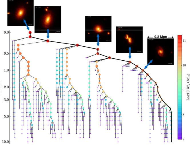
We construct galaxy merger trees by focusing on the stellar com-ponent of the subhalo merger trees. Fig.2shows such a tree for a galaxy withM∗=1.7×1011_M

atz=0, together with images of its star distribution highlighting its morphological evolution since

z=1. The main branch of the tree is marked by the thick black line. It is important to bear in mind that the identification of the main branch is always based on the branch mass; at any particular epoch, the most massive galaxy progenitor may not lie on the main branch. However, for the reasons described in Section 2.2.2, using the branch mass yields more stable and intuitive results.

Galaxy merger trees appear broadly similar to subhalo merger trees, except that the latter contain more fine branches corresponding to small subhaloes within which no stars have formed. Galaxy trees are also less affected by the mass exchange issue than subhalo trees, as star particles are more spatially concentrated.

2.3.3 Merger type

The effects of tidal forces and torques during a merger depend on the mass ratio of the merging systems (e.g. Barnes & Hernquist

1992). A merger between a low-mass satellite and a more massive host is generally less violent than a merger between systems of comparable mass, and has a less dramatic impact on the dynamics and morphology of the host. It is therefore useful to classify mergers into different types according to the mass ratio between the two merging systems,μ≡M2/M1(M1>M2). For galaxy mergers,μ is the ratio of stellar masses between two merging galaxies. While for halo mergers, it is the halo mass ratio.

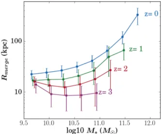
While this is straightforward in semi-analytic models (since galaxies are uniquely defined entities), in numerical simulations (and in nature as well), merging systems experience mass-loss due to tidal stripping throughout the merging process. Our strategy is therefore to choose a separation criterion, Rmerge, and determine the merger type when the merging systems are separated, for the first time, by that distance or less. For galaxy mergers, we adopt

Rmerge=5×R1/2, whereR1/2is the half-stellar mass radius of the primary galaxy (note thatRmergeis not a projected but a 3D separa-tion). The value ofRmergeranges from∼20 to 200 pkpc in the stellar mass range explored in this work (see Appendix A), and is similar to the projected separation criteria adopted in observational galaxy pair studies. For subhalo mergers,Rmerge=r200, wherer200is the radius of a region around the FoF group of the subhaloes within which the density is 200 times the cosmological critical density. In the rare event that an object is located within theRmergeof more than one other object, it is considered to be the merging companion of the nearest one.

Figure 2. An example of a galaxy merger history. The galaxy has a stellar massM∗=1.7×1011_M

at redshiftz=0. Symbol colours and sizes are logarithmically scaled with stellar mass. The thick solid line marks the main branch. The final galaxy is built from many small progenitors, but most of these contributors have very low mass. We also show images of its stellar mass distribution in a 200 comoving kpc box at a few redshifts. The galaxy shows prominent spiral-like structure at redshiftz=1, but then experiences several interactions with other objects, passing through a shell-like phase to transform into an elliptical galaxy atz=0.

(e.g. Rodriguez-Gomez et al.2015). Mergers with mass ratio≥1/4 can produce strong asymmetries in the morphology of both merging galaxies, making them easily identifiable in observations (Casteels et al.2014).

3 R E S U LT S

3.1 Galaxy formation and assembly time-scales

A simple way to summarize the formation history of a galaxy is to measure the time-scale on which it assembles its mass. As dis-cussed by De Lucia et al. (2006) and Neistein, van den Bosch & Dekel (2006), this can be assessed in two ways. First, we can mea-sure the total stellar mass in all progenitors of the final galaxy as a function of time. This mass increases through star formation. For many purposes, however, it is more relevant to focus on the growth of the main progenitor if we are interested in connecting galaxies identified in observational studies at different epochs. Following De Lucia et al. (2006), we refer to the time-scale by which the total mass of all progenitors has reached half of the stellar mass of the fi-nal galaxy as the ‘formation time’, tf. tf is closely related to the star formation history of the galaxy. The time-scale by which the main progenitor of the final galaxy has assembled that much mass is defined as the ‘assembly time’, ta. Both time-scales are

measured in lookback times. If a galaxy forms most of its stars throughin situstar formation, it will havetf≈ta,

Fig. 3 plots formation time,tf, against assembly time,ta, for galaxies atz=0 in three stellar mass bins. The galaxies occupy different regions in the plot depending on their stellar mass. Low-mass galaxies (M∗<1010.5_M

) typically formed their stars 8 Gyr ago. In spite of a large spread, their formation times scatter about the line ofta=tf, implying anin situorigin for their stars. In con-trast, the most massive galaxies formed their stars relatively early,

tf∼11 Gyr, and haveta<tfindicating that a fraction of their stars are formed elsewhere and subsequently assembled into the final sys-tem. The delay betweentaandtfis a strong function of galaxy mass, increasing rapidly as the galaxy mass exceeds 1011_M

. This trend agrees well with previous work (e.g. De Lucia et al.2006; Neistein et al.2006; Parry et al.2009). It is also seen in observational data, as a trend referred to as ‘downsizing’, where old stellar populations dominate massive galaxies (Bower, Lucey & Ellis1992; Cowie et al.1996; Heavens et al.2004; Gallazzi et al.2005) and low-mass galaxies have a more extended period of star formation (Noeske et al.2007; Leitner2012). These results hint that most low-mass galaxies that formed at high redshifts do not ‘survive’ to the present day and have merged into more massive galaxies. Indeed, we find that only half of the galaxies withM_∗∼109₋₁₀10.5_M

Figure 3. The formation time,tf, as a function of assembly time,ta, for galaxies atz=0. Both time-scales are measured as lookback times in Gyr, and the galaxies are classified into three bins of stellar mass by colours. The solid line represents the one to one relation for the two time-scales. Galaxies with stellar mass (M∗≤1010.5_M

), are distributed along this line, indicating that they assemble most of their stars throughin situstar formation. In massive galaxies ofM∗>1011_M

, by contrast,talags behind

tf, and the galaxies are offset from theta=tfline, showing the importance of stars formed in other objects and subsequently accreted. The normalized histograms of thetfandtadistributions are shown in marginal panels. The mean and the median of the distributions are indicated by the solid and dotted lines, respectively.

In aCDM universe, dark matter haloes grow in a self-similar manner, with high-mass haloes typically being formed more re-cently than their low-mass counterparts (Davis et al.1985; Bardeen et al.1986). This is confirmed in Fig.4, which shows the distri-bution oftaas a function oftf for the haloes hosting the galaxies of Fig.3. Points are again coloured by the present-day stellar mass of the galaxies, as in Fig.3. We see that both time-scales decrease with increasing halo mass, as expected from the hierarchical struc-ture formation scenario. This is entirely the opposite trend to that seen for the galaxies.

This apparent contradiction is the result of AGN feedback being more effective in high-mass haloes (Bower et al.2006). At low mass, stellar feedback causes the galaxy’s stellar mass to scale with approximately the square of the halo mass, so that the galaxies grow rapidly as the halo mass increases. The stars gained by accretion and merging are dwarfed by the contribution from ongoing star formation. However, once the halo mass exceeds∼1011.5_M

, star formation is strongly suppressed by AGN feedback (see Rosas-Guevara et al.2015, and Bower et al.2016) and galaxies grow almost exclusively by accretion and mergers. This transition breaks any self-similarity in the hierarchy: although the most massive galaxies assemble late, the stars they contain were formed at much earlier epochs.

The halo assembly and formation times are remarkably close. This occurs because the dominant contribution to halo growth comes from matter which is not yet bound into galaxy-bearing dark matter haloes. Many previous studies have pointed out that in a CDM cosmology, halo growth is driven by a mix of mergers and accretion

Figure 4. Formation and assembly times for the parent dark matter halo of the galaxies shown in Fig3. Note that haloes are binned by the stellar mass of their central galaxy, but that bins of higher stellar mass correspond to higher mean halo mass. The solid line represents the case wheretf=ta, as in Fig3. In contrast to the situation for galaxies,tfandtaincrease with decreasing stellar mass, demonstrating the hierarchical nature of the mass assembly of dark matter haloes. Note, however, that formation and assembly times are similar regardless of mass, meaning that halo growth is dominated by accretion of diffuse material. The assembly histories of haloes are markedly different from those of the galaxies they contain.

of matter that has not yet collapsed into identifiable haloes (e.g. Kauffmann & White 1993; Lacey & Cole1993; Guo & White

2008; Fakhouri & Ma2010; Genel et al.2010; Wang et al.2011). In contrast, stars are only formed efficiently in well-defined massive haloes. This fundamental differences results in the stark contrast between Figs3and4.

3.2 The redshift evolution of galaxy formation and assembly times

In previous section, we have shown that the delay between formation time and assembly time can provide some useful hints on how a galaxy assembles its mass. In this section, we use the differences of both time-scales as a tool to examine the assembly history of galaxies at different redshifts.

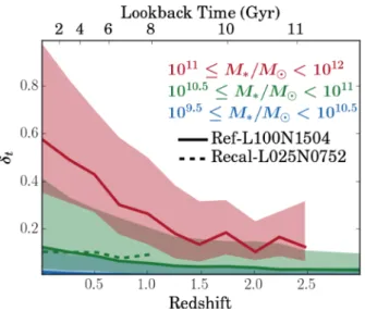
To quantity the relative difference between the two time-scales, we define a dimensionless parameter,

δt≡1−tf/ta.

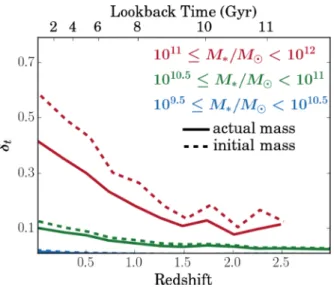
Figure 5. The evolution of the relative difference between the assembly and formation times,δt, for galaxies in three stellar mass bins (indicated by colour and legend). Lines represent the medians of theδtdistributions. The shaded regions enclose the 25th–75th percentiles. Bins with fewer than 10 galaxies are not shown.δtincreases with stellar mass but decreases with redshift, showing the importance of external processes in the mass assembly of low-redshift massive galaxies. These trends are insensitive to resolution, as shown by the agreement between the results of Ref-L100N1504 (solid lines) and of Recal-L025N0752 (dashed lines), although the latter simulation lacks objects in the highest mass bin.

results from the much higher specific star formation rates of high-redshift galaxies due (at least in part) to the higher gas infall rates and the less efficient AGN feedback of young galaxies.

We should note that both time-scales are calculated using the actual (observed) stellar masses of galaxies, not the stellar masses initially formed. Because using the latter assigns greater weight to old stars and results in earlier formation and assembly times. In practice, however, the change affects the two time-scales in a similar manner (see Appendix B for detailed discussion) and thus does not change the overall result.

3.3 The contribution of star formation in external galaxies

Time-scale studies shed light on the manner in which galaxies with different masses at different redshifts aggregate their stars. But they do not explore quantitatively the roles of internal and external pro-cesses therein. In this section, we evaluate the relative importance of those processes by their mass contributions to galaxy assembly. To avoid the mass-loss from stellar evolution, we use initial stellar masses in the calculation.

For each of our samples, we first trace back along the main branch of its merger tree to identify when the main progenitor was involved in a merger event (i.e. mass ratioμ≥1/10) or accretion (μ <1/10) events. We consider the stellar mass of the infalling object at the start of the event (i.e. when the merger type is determined) to be the mass contribution of that event, under the assumption that all the stars of the object will be accreted by the primary host. We sum up the mass that a galaxy has acquired from mergers and accretion, and derive the fractional contribution of external pro-cesses,fext, by comparing this mass to the final galaxy mass. Tidally induced shocks and angular momentum loss during a merging pro-cess can trigger bursts of star formation, contributing to galaxy mass

build-up. In our calculation, this mass gain is regarded as part of the contribution fromin situstar formation.

Fig.6showsfextof low-, intermediate-, and high-mass galaxies from redshiftz=0 to 3. Lines show the median values, while the shaded regions represent the 25th–75th percentiles of the distribu-tion. Both results of the reference Ref-L100N1504 (solid lines) and the higher resolution Recal-L025N0752 (dashed lines) simulations are shown in order to demonstrate the convergence of the results. The low-mass galaxies at redshiftz=0 acquire only a small frac-tion of their mass from external galaxies. Over the explored redshift range, the median contribution is∼0.1 with very little evolution. In contrast, galaxies in high-mass bin receive the greatest fractional contribution from mergers and accretion in terms of stellar mass gain, with a median of∼0.19 and a 75th percentile of∼0.39. This fraction declines with redshift to∼0.08 atz=2.5. Nevertheless, the low values offextfor galaxies of any mass at both low- and high-redshifts highlight the relative importance ofin situstar formation with respect to external processes to the assembly of galaxies.

3.4 Galaxy merging history

In preceding sections, we explored the relative roles thatin situ

and external star formation play in galaxy mass build-up. In this section, we continue our investigation by exploring the separate contributions of the different external processes in galaxy assem-bly. According to the mass ratio between the two merging systems (μ =M2/M1whereM1 >M2), these processes are divided into major mergers (μ≥1/4), minor mergers (1/4> μ≥1/10), and accretion (μ <1/10).

3.4.1 Redshift of last major merger

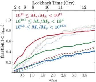
Almost all of our present-day galaxies, irrespective of their stellar mass, have experienced at least one major merger event in their lives. We use the merger trees to determine the redshift,zlast, when they experienced their last major merger. Fig.7shows the cumulative distribution ofzlastfor galaxies in three stellar mass bins. The most massive galaxies have a very active merging history, with 68 per cent of the population having been involved in a major merger event since

z=1.5 (a lookback time of 10 Gyr). This fraction declines with decreasing galaxy mass and drops to 41 per cent for intermediate-mass galaxies, and further down to 22 per cent for the least intermediate-massive galaxies.

Observations of the stellar dynamics of the Milky Way galaxy suggest that no major mergers have occurred in the last 10 Gyr (Ruchti et al.2015). Our results show that there is no tension be-tween the quiet history of the Milky Way and the CDM paradigm. The Milky Way could easily have been drawn from the∼60 per cent of the population that has not undergone a major merger. The merger history inferred from the fossil record of the Milky Way is therefore not in conflict with those of similar mass galaxies in the EAGLE simulations.

For comparison, Fig.7also shows the cumulative distributions of

Figure 6. The initial stellar mass contributions of mergers (i.e. mass ratioμ≥1/10) and diffuse accretion (μ <1/10) for galaxies of different stellar mass, at redshiftsz=0–3 in three stellar mass bins (as coloured). Solid and dashed lines represent the median of the distribution in Ref-L100N1504 and Recal-L025N0752, respectively. Our analysis stops at the redshift when fewer than 10 galaxies are available. The shaded regions bracket the 25th and the 75th percentiles of the distributions. External mass contributions increase with galaxy stellar mass but decrease with redshift.

Figure 7. The cumulative distribution of the redshift of the last major merger event (μ≥1/4),zlast, for present-day galaxies (solid lines) and their parent subhaloes (dashed lines). Galaxies are split into three stellar mass bins as labelled. Only 22 per cent of galaxies withM∗<1010.5_M

have experienced a major merger event atz<1.5. In contrast, 68 per cent of the most massive galaxies have experienced many recent merger events. This mass dependence is not seen in thezlast distribution of their parent subhaloes, which is due to the non-linear dependence of stellar mass on halo mass. While the distribution for major subhalo mergers is similar to that of low-mass galaxies, the subhalozlastdistribution looks more similar to that of high-mass galaxies when minor halo mergers are included (dotted lines).

intermediate-mass bin, very recent major mergers between galaxies outnumber those of subhaloes by about 10 per cent–15 per cent. This comparison highlights the important difference between the merger classification of galaxies and those of subhaloes, especially the massive ones. In the high-mass range, the mild dependence of the stellar mass on halo mass (M_∗∝M_h1/2) means that merging galaxies closely matched in mass may have subhaloes of quite different masses. Dotted lines in Fig.7 show the distribution of zlast for subhaloes when minor halo mergers are also taken into account. As expected, these lines are much more similar to thezlastdistribution of major mergers of massive galaxies.

3.4.2 The contributions of major mergers, minor mergers, and accretion

In this section, we continue our investigation of fractional mass contribution in Section 3.3 further to explore the respective contri-butions from major merger, minor merger and accretion and their dependence on galaxy mass and redshift. As in Section 3.3, the initial stellar masses of galaxies are used in the calculation in order to remove the impact of stellar evolution-induced mass-loss.

As the fractional mass contributions show large scatter due to the wide variety of galaxy merging histories, we calculate the fraction of galaxies receiving at least a given fractional mass contribution from each process. The panels from left to right in Fig.8show the cumulative fraction of galaxies at redshiftz=0 (solid lines), 1 (dashed lines), and 2 (dotted lines) as a function of the minimum fractional mass contribution from major mergers, minor mergers and accretion, respectively. As before, galaxies are binned into low-(blue), intermediate- (green), and high-mass (red) bins. Low-mass galaxies at redshift z = 0 mainly acquire their external masses through accretion, while major mergers are the main contributor for their high-mass counterparts. Around∼61 per cent of the most massive population acquired more than half of their external mass through major merger events. Parry et al. (2009) arrived at the same conclusion from their analysis of semi-analytic models in the Millennium simulation (see fig. 8 in their work). This shift in behaviour is driven by the shallow dependence of stellar mass on halo mass at high halo masses. SinceM_∗∝M_h1/2, a wide range of halo mass ratios lead to mergers occurring between galaxies of comparable mass.

Nevertheless, the role of major mergers diminishes with increas-ing redshift, and at the same time, accretion plays a larger role towards higher redshift. As our results show, at redshift z = 2, galaxies of any mass acquired most of their external mass through accretion.

3.4.3 Evolution of the galaxy merger fraction

Figure 8. The fraction of galaxies as a function of the minimum external stellar mass contributed by major mergers (μ≥1/4, left-hand panel), minor mergers (1/4> μ≥1/10, middle panel) and accretion (μ <1/10, right-hand panel) at redshiftz=0 (solid lines), 1 (dashed lines), and 2 ( dotted lines). The galaxies are split into three bins of stellar mass coded by colours. While accretion plays a larger role than mergers in terms of the external stellar mass contribution in low- and intermediate-mass galaxies, at low redshift, major mergers dominate the external mass contribution in the most massive galaxies.

We search galaxy merger trees for galaxies appearing in pairs at each snapshot. These pairs are subject to selection criteria somewhat similar to those applied to the observational close-pair studies. Any two galaxies are classified as a merging pair if they: are separated by a distance≤Rmerg(Rmergis five times the half-stellar mass radius of the primary galaxy, see Section 2.3.3); have a mass ratioμ≥ 1/4; share a common future descendant. The last criterion frees our major merger census from the interference of random line-of-sight alignments.

If two galaxies have not finished merging byz=0, they will not appear in the same merger tree because they do not have a common descendant. As a result, they will not be considered to be a merger pair. Kitzbichler & White (2008) show that the merging times of galaxy pairs can be very extended, leading to a large fraction of pairs surviving toz=0. To include these pairs in the merger fraction calculation, one should go further in time to construct their merging histories afterz=0. However, as our results show later, neglecting the unfinished pairs has only a trivial impact on the global merger fraction.

We count the number of galaxies that are in pairs. When a galaxy is paired with more than one secondary galaxy, the primary galaxy is counted only once. The galaxy merger fraction is derived by dividing this number by the total number of galaxies at that snapshot. A merger fraction can be converted into a merger rate if we know the merger time-scale. The time intervals between EAGLE snapshot outputs typically ranges from 0.1 to∼1 Gyr and may thus not suffice to derive an accurate estimate of the merger rate. We therefore focus on the galaxy merger fraction, rather than the merger rate. Our approach is more readily compared to observational measurements (although caution is still warranted because we have not attempted to account for observational biases).

Fig.9shows the major merger fraction,fmerge, for galaxies with stellar massM_∗≥109.5_M

(black dots),M_∗≥1010.5_M (blue dots), andM∗≥1011_M

(red dots) over redshiftz =0–4. The galaxy merger fraction increases monotonically towards high red-shifts before levelling off at z 1–3, depending on mass. The

fmergeof galaxies withM∗≥1011Meven declines forz>2. We compare the simulation predictions with a compilation of real data from both galaxy close-pair studies (open symbols; Kartaltepe et al.

2007; Lin et al. 2008; Ryan et al. 2008; De Ravel et al.2009; Williams et al.2011; Man et al.2014) and galaxy merger studies based on morphological diagnostics (solid symbols) like the CAS

Figure 9. Major merger fraction as a function of redshift for galax-ies withM∗≥109.5_M

(black circles),≥1010.5_M

(blue circles), and M∗≥1011_M

(red circles) derived from Ref-L100N1504. The simula-tion predicsimula-tions lie within the scatter of the observasimula-tional data from both close-pair studies (solid grey symbols) and morphological diagnostics ( open grey symbols). Curves represent power-law/exponential fits to the simulated merger fraction in the corresponding stellar mass bins.

(Conselice et al.2009) or the Gini/M20 (Conselice, Rajgor & Myers

2008; Lotz et al.2008; Stott et al.2013). These data are mostly for galaxies withM_∗≥1010_M

. Note that this comparison is qual-itative since a detailed comparison would require careful recon-struction of the observational criteria. Overall, however, the pre-dicted galaxy merger fraction lies within the scatter of observational data, but is most compatible with studies based on morphological analysis.

Observational studies often parametrize the redshift dependence of the galaxy merger fraction as a power law,∝(1+z)n_{, with index}

n=0–4. However, the rise of the merger fraction beyond redshift

Table 1. The values of the parametersa,b,c, with 1σ uncertainties, of a power-law/exponential fitting functiona(1+z)b_ec(1+z) _{in which zis} redshift. These values are determined by the least-square fittings to the predicted galaxy merger fraction in three stellar mass bins.

M∗/M a b c

≥1010 _{0.035±0.069 3.694±0.519 0.771±0.206} ≥1010.5 _{0.062±0.074 3.206±0.560 0.801±0.222} ≥1011 _{0.122±0.422 2.833±2.433 0.889±1.195}

in Fig.9represent the least-square fitting results in three mass bins. Table1lists the best-fitting values of the three parameters and their 1σ uncertainties obtained from the fitting.

The merger diagnostics are also sensitive to merger mass ratios, we also consider the impact on our results of extending the merger mass ratio to a smaller value (μ≥1/10). We find that the merger fraction is elevated by only a factor of 1.5–1.8, on average, by the inclusion of minor merging events, and shows similar trends with redshift.

3.5 The impact of feedback on galaxy mass assembly

So far, we have shown that the assembly of massive galaxies is very different to that of their smaller counterparts. A very interesting question is whether this is due to the feedback from star formation and black hole growth. AGN feedback, for example, is able to efficiently suppressin situstar formation by heating the hot coronae of galaxies and suppressing the inflow of cool gas (Bower et al.

2016). To gain more insight on this aspect, we calculate the mass contribution of internal and external processes in simulations with varying efficiencies of feedback from stars and AGN. These runs differ in simulation volume but have the same resolution. Table2

lists the values of the parameters used in their feedback models. The effect of these changes on the stellar mass function and galaxy star formation rates is considered in Crain et al. (2015).

The panels from left to right in Fig. 10 compare the frac-tional mass contribution from mergers and accretion,fext, for low-, intermediate-, and high-mass galaxies over redshiftz=0–3 in the presence of weak (dot–dashed lines) and strong (dashed lines) stel-lar feedback, and no AGN feedback (dotted lines). The results for the reference model (solid lines) are also shown for comparison. The lines show the median of thefextdistribution and stop at the redshift when fewer than 10 galaxies are available for analysis. We find that stellar feedback has very limited impact on the mass build-up of low-mass galaxies (left-hand panel). Increasing or decreasing the feedback efficiency leads to only5 per cent of changes in their

fext. In the strong feedback case, the analysis consistently suggests a slight decrease offext as more of the star-forming gas within

small galaxies is lost in outflows, reducing their contribution to the stellar mass. The formation of massive galaxies is also strongly suppressed, however, and the small simulation volume (25 cMpc) prevents us reliably determining if there is an increase infextin the few large objects that form. In the case of weak stellar feedback, the efficiency of galaxy formation is similarly increased over a wider range of halo mass, andfextchanges little in the left-hand panel. In the middle panel,fextis lower than the reference simulation (and is more similar to the curve in the left-hand panel). In the absence of effective stellar feedback, AGN feedback has a similar impact in high- and low-mass haloes (Bower et al.2016) and we expect the differences between the panels to be smaller, as seen.

Galaxies in the first two panels are insensitive to the AGN feed-back since (in the reference model) star formation driven outflows oppose the build-up of high gas densities in the central regions (Bower et al.2016). In contrast, the AGN feedback has a very no-ticeable impact on thefextof their massive counterparts.fextdeclines in the absence of AGN feedback, consistent with the negative im-pact of AGN feedback onin situstar forming in massive galaxies. This explains many of the differences, but not all of them. For ex-ample, for the most massive galaxies, there is still a rapid rise infext to the present day that may be related to the recent cosmological acceleration of the Universe.

4 C O M PA R I S O N S T O OT H E R W O R K

In this work, we focus on the assembly and formation of galaxies. This is a topic that has been extensively studied using N-body simulations and semi-analytic galaxy formation models.

Kauffmann, Charlot & White (1996) and De Lucia et al. (2006) already show that the formation time of brightest cluster galaxies is much earlier than their assembly time and Parry et al. (2009) show that with the exception of the brightest galaxies, major mergers are not the primary mechanism by which most galaxies assemble their mass. Our hydrodynamic EAGLE simulations exhibit the same trends and their dynamic range allows us to contrast the formation of the most massive galaxies with that of galaxies similar to the Milky Way. We do not, however, find galaxies with formation and assembly times as large as in De Lucia & Blaizot (2007), who find that galaxies withM∗>1012_M

form 50 per cent of their stars atz≈5; galaxies in our highest mass bin only cover the range of 1011_–1012_M

and form most of their stars atz>2.

Guo & White (2008) compare the contributions from star for-mation and galaxy mergers to the mass build-up of galaxies using semi-analytical models. In common with our results, they find that major merger play an important role in the growth of galaxies more massive than the Milky Way and that the relative importance of star formation increases towards high redshift. Nevertheless, we dis-agree with their conclusion about major mergers also dominating

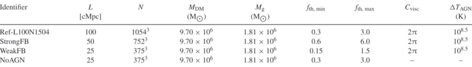
Table 2. Values of the parameters used in the simulations with varying feedback efficiency: size of the simulation volume (L), particle number (N), dark matter and initial baryonic particle mass (MDMandMg), the asymptotic minimum and maximum value of stellar feedback efficiency (fth, minandfth, max), accretion disc viscosityCvisc, and the temperature increment of stochastic AGN heating (TAGN). We refer readers to Crain et al. (2015) for detailed information on

these paramertes.

Identifier L N MDM Mg fth, min fth, max Cvisc TAGN

[cMpc] (M) (M) (K)

Ref-L100N1504 100 10543 _9.70×106 _1.81×106 _{0.3 3.0 2π 10}8.5

StrongFB 50 7523 _9.70×106 _1.81×106 _{0.6 6.0 2π 10}8.5

WeakFB 25 3753 _9.70×106 _1.81×106 _{0.15 1.5 2π 10}8.5

Figure 10. The fractional mass contribution of mergers and accretion for galaxies at redshiftsz=0–3 when there is strong (dashed lines) and weak (dash– dotted) stellar feedback, and no AGN feedback (dotted lines). The reference model (solid lines) is also shown for comparison. We split the galaxies into three stellar mass bins. We only show points for which more than 10 galaxies contribute. Changes in the efficiency of star formation and the role of AGN make significant differences to the external stellar mass fraction.

the growth of high-redshift massive galaxies. Our results show that

in situstar formation, instead of major mergers, is the dominant contributor to those galaxies.

Lackner et al. (2012) examine galaxy formation and assembly histories in adaptive mesh refinement simulations. Their results show that the accreted fraction has a smooth dependence on stel-lar mass, but their calculations do not include AGN feedback and do not capture the observed break in the galaxy stellar mass func-tion. The importance of feedback can be recognized by looking at zoomed simulations of galaxies similar to the Milky Way. Our results disagree with the high accreted star contributions reported by Oser et al. (2010). This discrepancy is presumably due to the lack of effective feedback at high redshift in their runs, as thein situfraction can be drastically reduced in simulations without any feedback (Hirschmann et al.2012).

Rodriguez-Gomez et al. (2016) also provide some insight on this topic using the Illustris simulation (Vogelsberger et al.2014). Similar to our results, they confirm the greater role of mergers and accretion in the mass growth of present-day massive galaxies withM_∗>1011_M

as well as the decreasing importance of these processes with increasing redshift. This similarity supports the ro-bustness of our conclusions to varying subgrid physical models. In particular, we make a comparison between the results with vary-ing feedback efficiencies, sheddvary-ing light on how stellar and AGN feedback affect the mass build-up of galaxies. Nevertheless, there is also disagreement between our results and that of Rodriguez-Gomez et al. (2016). They highlight the importance of major merg-ers in contributing to the assembly of low-mass galaxies and high-mass galaxies alike. This contrasts with our results which show that accretion, rather than major mergers, are the main contribu-tors in low-mass galaxies. This discrepancy may be the result of the different methods the two works used for merger type determi-nation. While Rodriguez-Gomez et al. (2016) define the type of a merger event when the secondary galaxy reaches its maximum stel-lar mass, we determine the merger type when the secondary galaxy is some distance, five times the half-stellar mass radius of the primary galaxy, from the primary host. Unfortunately, the time interval of the EAGLE snapshot outputs is not sufficient to demonstrate that the two methods look at the same merging epoch and classify the merg-ers in the same way. It is also worth noting that the mass-loss from stellar evolution is taken into account in our mass contribution

calculation and that Illustris simulation has a steeper slope to the faint-end galaxy mass function, compared to our simulation and observations. The most fundamental difference may, however, be the implementation of stellar and AGN feedback. These are very different in the simulations, and we have shown that this can lead to significant differences in galaxy assembly histories in Section 3.5. Clearly, this is an interesting avenue for more detailed future inves-tigation.

Moster et al. (2013) and Behroozi et al. (2013) consider the topic from a more observational perspective, using the abundance match-ing method. They find increasmatch-ing trends in the fraction of accreted stars with increasing galaxy mass and decreasing redshift that agree closely with our simulations. The consistency between the empirical results and the simulation predictions provides encouraging support both to our results and to the EAGLE simulation runs.

Our results show that the mass assembly of galaxies, however, is not simply a reflection of the growth of their parent haloes. Addi-tional physical processes, such as stellar and AGN feedback, make galaxy formation efficiency a strong function of halo mass Mh. The resulting stellar mass–halo mass relation has a steep slope in low-mass haloes (M∗∝Mh2) and a shallower slope at high mass (∝M1/2

h ) (e.g. Benson et al.2003). The steep low-mass slope arises because the binding energy per unit mass of the halo scales with the halo mass asMh5/3, while the energy available from stars is propor-tional to the stellar mass. The high-mass slope arises because AGN feedback is able to suppress star formation and because the cooling time is long in massive haloes (e.g. Rees1977; Silk & Rees1998; Benson et al.2003; Bower et al.2006; Croton et al.2006), leav-ing galaxy mergleav-ing as the only effective growth channel. From an observational perspective, the connection can be derived by match-ing the abundance of galaxies and haloes assummatch-ing a monotonic relation (e.g. Kravtsov et al.2004). The dark matter mass function is described as a power law (with index∼−1) with only a slow rollover at high mass. In contrast, the galaxy stellar mass function is almost flat at low mass (e.g. Fontana et al.2006). Matching the two by abundance requires a quadratic dependence of stellar mass on halo mass. At high mass, the galaxy stellar mass function has a sharp break implying that haloes of increasing mass host galaxies of very similar mass.

and halo mass-dependent (e.g. Cattaneo et al.2011). For low-mass galaxies and haloes, a halo merger with a mass ratio 1/4 may corre-spond (roughly) to a merger between galaxies of mass∼1/16. For massive galaxies, a minor halo merger (between a massive halo and a satellite halo) may actually correspond to a major (almost equal-mass) galaxy merger. In this high-mass regime, assuming a uniform galaxy formation efficiency to derive galaxy merging histories from halo merging histories inevitably underestimates the importance of major galaxy mergers, and overstates the role of minor mergers. Many papers have pointed out the disagreement between the galaxy merger rate and the halo merger rate (e.g. Berrier et al.2006; Parry et al.2009; Hopkins et al.2010; Guo et al.2011), and here we are able to demonstrate this directly. We compare the times (in redshift,

zlast) when galaxies and their parent subhaloes experience their last major merger events, and find that thezlastdistribution of massive galaxies differs greatly from that of their host subhaloes. The former looks more closely like thezlastdistribution of subhaloes only when minor subhalo mergers are also included.

The principal aim of this paper has been to quantify the role of mergers in the formation histories of galaxies in the EAGLE refer-ence simulation. Since the simulation provides a good description of the galaxy stellar mass function and its evolution, as well as many other aspects of the observable Universe, we make the im-plicit assumption that the formation histories of the simulated galax-ies provide a good approximation to those of galaxgalax-ies in the real Universe. The long time-scales of galaxy evolution make it im-possible to observe the growth of galaxies directly; nevertheless, it may be possible to reconstruct the build-up of one galaxy, the Milky Way, from careful archaeology of its stellar content, and their the use of chemical tagging techniques (Hogg et al.2016). Unfortunately, the formation history of galaxies like the Milky Way is extremely diverse, and careful thought will be required to understand how results, such as those from theGaiasatellite, can be used to reach definitive conclusions.

5 S U M M A RY A N D C O N C L U S I O N S

In this paper, we have investigated the assembly and merging his-tories of hundreds of thousands of central galaxies in the EAGLE cosmological simulation project. The hydrodynamic simulations include a range of gas, stellar and black hole physical processes relevant to galaxy formation, and have been shown to match the properties of observed galaxies reasonably well. Because of this, these simulations provide an ideal test bed for elucidating the roles played by galaxy mergers andin situ star formation in galaxy formation.

We construct galaxy merger trees by applying the D-Trees algo-rithm (Jiang et al.2014) to SUBFIND subhalo catalogues across snapshot outputs. They enable us to chronicle galaxy formation fromz=3 to the present day. Because galaxies will slowly lose stellar mass due to tidal stripping before they finally merge, a care-ful definition of the masses of galaxies prior to and during a merger is required. In this paper, we use a definition based on a separation of five times the galaxy half-stellar mass radius to signal the start of a merging event and then determine the merger type. According to the mass ratio between the primary and the secondary galaxies, merger events are classified as either major mergers (with mass ratiosμ≥1/4), minor mergers (1/4> μ≥1/10), or accretion (μ <1/10). Considering that galaxies also suffer mass-loss due to stellar evolution, we use the initial stellar mass, i.e. the stellar mass being formed, when evaluating the relative contributions ofin situ

and external processes to the mass growth of galaxies.

Our main results are summarized as follows.

(i) We contrast the assembly time (ta, when the main progenitor of a galaxy had assembled half its present-day stellar mass) and the formation time (tf, when that mass had formed, regardless in which progenitor) of galaxies. Galaxies less massive than 1010.5_M

have very similartfandta, showing that most of their stars formed in their main progenitors. Above a mass of 1010.5_M

, galaxies are domi-nated by increasingly old stars, but for the most massive galaxies, the assembly time decreases, implying that although the stars are old, they have only recently been assembled into the present-day galaxies (Fig. 3). We also compare the formation and assembly times of galaxies with those of their parent subhaloes and find quite different trends. Thetf andta of the subhaloes, in contrast, show a high level of similarity over the mass range studied, decreasing monotonically with increasing mass (Fig.4).

(ii) We quantify the mass fraction of stars that are formed ‘in situ’ versus stars that have an accreted origin. Galaxies less massive than 1010.5_M

typically acquire less than 10 per cent of their mass through galaxy mergers or accretion of stars formed in other sys-tems. In contrast, in galaxies more massive than 1011_M

, typically ∼20 per cent of the system’s stars have an external origin. There is considerable scatter in both cases (Fig.6).

(iii) The fraction of accreted stellar mass in less massive galax-ies evolves mildly with redshift. In the high-mass galaxgalax-ies, the assembly and formation times become increasingly similar with in-creasing redshift and the fraction of externally formed stellar mass declines (Figs5and6).

(iv) We measure the distribution of the redshifts when galaxies have their last major mergers. For galaxies less massive than the Milky Way, the median redshift of the last major merger isz≈2, which is compatible with the quiet formation history of the Milky Way implied by recent observations (Fig.7).

(v) Accretion dominates the external mass contribution for less massive galaxies, while major mergers become the main mass con-tributor of external mass for massive galaxies (Fig.8).

(vi) We compute the fraction of galaxies in a snapshot that are undergoing major mergers, and explore the variation of this frac-tion with redshift and galaxy mass. We find that the merger fracfrac-tion rises rapidly between the redshiftsz=0 and 1, but flattens at higher redshift. Given the uncertainties inherent in the comparison, and the range of methods applied to observational data sets to this diagnos-tic, our simulation predictions display a remarkable similarity with observational studies (Fig.9).

(vii) Strengthening or weakening stellar feedback results in a decline in the external mass contribution to galaxies. While low-mass galaxies are weakly affected by AGN feedback, their low-massive counterparts show a significant reduction in the external mass con-tribution (Fig.10). These changes can be broadly understood as resulting from changes in the efficiency of ongoing star formation and the impact of AGN feedback.

Overall, we find general agreement between our results and stud-ies based on semi-analytic models. Massive galaxstud-ies are found to have started their star formation earlier than low-mass galaxies but partly in objects other than the main progenitor, and then bled those stars later through mergers and accretion. This assem-bly history also implies that they have older stellar populations, consistent with the ‘downsizing’ trend seen in many observational studies.