Journal archive

(1)

HYPERION

INTERNATIONAL

JOURNAL

(2)

(3)

Hyperion International Journal of Econophysics & New Economy

MODELING THE REASONS FOR FIRMS'

GROWTH: A CONTROL-THEORETIC APPROACH

Matti ESTOLA*

Abstract. Static neoclassical framework cannot be applied in modeling time dependent processes or increasing returns to scale in production. The dynamization of the neoclassical theory of a firm by dynamic optimization, on the other hand, assumes inconsistent profit functions with the former. As a solution to these problems, we present a dynamic theory of a firm consistent with the static neoclassical one. A firm's growth may originate from increasing demand or decreasing costs with time, or increasing returns to scale in production (Estola 2001). We model the reasons causing increasing returns in a firm’s production process and give a block diagram of the model to reveal its control theoretic nature. (JEL B41, D21, D24)

Keywords: Dynamics, firms' growth, control theory, block diagram.

1. Introduction

According to Philip Mirowski (1989a), neoclassical economics bases on two distinct elements: egoistic economic agents by Adam Smith (utility maximizing consumers by William Stanley Jevons, Carl Menger and Leon Walras) and the mathematical metaphor of classical mechanics. The latter can be understood by the progenitors of the neoclassical theory who were engineer level physicists. Concept equilibrium in economics was borrowed from physics by Nicolas-Francois Canard at 1801 (Mirowski 1989b). Although equilibrium is a balance of forces situation, in economics the balancing forces have not been defined. However, to understand the adjustment process we should define the forces that ‘push’ economic quantities into their equilibrium states in stable cases, or cause their evolution with time in non-stable cases.

The existence of forces acting upon economic quantities can be argued indirectly; every changing quantity (price, wage, exchange rate etc.) tells the existence of reasons (forces) causing these changes. This is analogous with arguing the existence of the gravitational force field by dropping a pen; without the force field the pen would not move. Franklin

*

(8)

M. Fisher (1983 pp. 9-12) writes: “... I now briefly consider the features that a proper theory of disequilibrium adjustment should have ... if we are to show under what conditions the rational behavior of individual agents drives an economy to equilibrium. ... Such a theory must involve dynamics with adjustment to disequilibrium over time modeled. ...the most satisfactory situation would be one in which the equations of motion of the system permitted an explicit solution with the values of all the variables given as specific, known functions of time. ... Unfortunately, such a closed-form solution is far too much to hope for. ...the theory of the household and the firm must be reformulated and extended where necessary to allow agents to perceive that the economy is not in equilibrium and to act on that perception. ... A convergence theory that is to provide a satisfactory underpinning for equilibrium analysis must be a theory in which the adjustments to disequilibrium made by agents are made optimally”.

According to Kenneth Arrow & Frank Hahn (1971, p. 12), the accepted definition for market stability is that of Paul Samuelson (1942) who writes: “In the history of mechanics, the theory of statics was developed before the dynamical problem was even formulated. But the problem of stability of equilibrium cannot be discussed except with reference to dynamical considerations ... we must first develop a theory of dynamics”. Andreu Mas-Colell et al. (1995, p. 620) write: “A characteristic feature that distinguishes economics from other scientific fields is that, for us, the equations of equilibrium constitute the center of our discipline. Other sciences, such as physics or even ecology, put comparatively more emphasis on the determination of dynamic laws of change. The reason, informally speaking, is that economists are good (or so we hope) at recognizing a state of equilibrium but are poor at predicting precisely how an economy in disequilibrium will evolve. Certainly there are intuitive dynamic principles: if demand is larger than supply then price will increase, if price is larger than marginal costs then production will expand”.

2. Dynamic Control Theoretic Model

(9)

like to better the firm's situation if possible, as Fisher stated above. We believe that ‘economic agents’ desire to better their situation’ is the fundamental cause for the observed dynamics in economies.

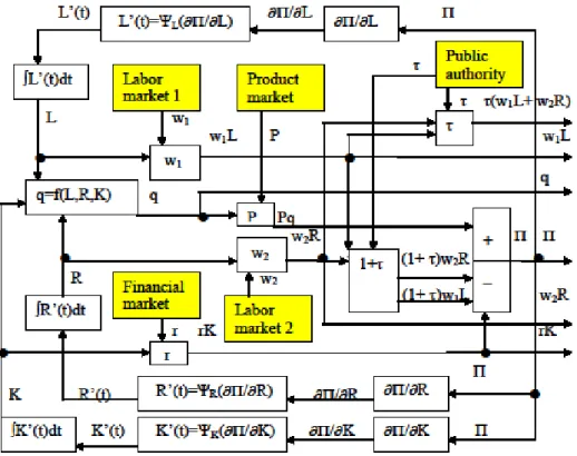
Dynamic control theoretic models of firms’ behavior completely base on dynamic optimization; see Alain Bensoussan et al. (1974) or Alpha C. Chiang (1992). In physics, however, Hamilton's and Newton's modeling principles yield the same equations of motion, and Newton's method applies differential equations while Hamilton's principle requires dynamic optimization. Due to this relative simplicity, most engineering applications of control theory rely on Newton's principle. In engineering models it is also common to present a block diagram of a system before its behavior is analyzed formally (see S. A. Marshall (1978) or Katsuhiko Ogata (1997)). We propose a similar simplification for control theoretic modeling in economics as Newton's principle offers in physics. The force vector that causes the dynamics of use of every input of a firm guides the firm with time into its profit maximizing state, and so dynamic optimization is not needed. The Newtonian type of a dynamic law for the firm's adjustment of its use of inputs is used as a building block in our model as is common in engineering (see Fig. 1). By the model we study the reasons for production dynamics at firm level.

(10)

In Figure 1, the ‘flows’ denoted by arrows are named by the ‘flowing’ quantities. Symbol • means that the crossing ‘flows’ are connected, that is, the same flow is in both lines; otherwise crossing lines are assumed not to interact with each other. White rectangles affect the ‘flows’ as is shown, and yellow rectangles of external impulses to the system. For every rectangle, the input and output flows are named. In the single [+/–] – box, the monetary flow entering the upper part is added with a positive sign, and those entering the lower part are added with a negative sign. The output flow from this box is the profit Π. The diagram shows how profit-seeking, the ultimate goal of the firm, controls the production process. All three inputs in the production are adjusted by a closed-loop mechanism where the feed-back bases on the marginal profitability of the input. The real output of the system is q, and the monetary outputs are and for the two types of labor,

L

w₁ w₂R

) (w₁L+w₂R

τ for the government, rK for the lenders of foreign capital or investors of own capital, and Π to the firm’s owners. The main definitions are:

), , , (L R K f

q = Π = Pq−(1+τ)w₁L−(1+τ)w₂R−rK,

; ) 1 ( ) / (

/∂L=P ∂f ∂L − +τ w₁

Π

∂ ∂Π/∂R = P(∂f /∂R)−(1+τ)w₂,

, ) / (

/∂K = P ∂f ∂K −r

Π

∂ x'(t)=Ψ_x(∂Π/∂x), x= L,R,K.

(11)

3. Kinematics of Production

We denote by (unit/y) the flow of production of a firm at time moment t. Unit may be one day, two weeks etc. The accumulated produc-tion of the firm till time moment t, is:

) (t q y ), ( ) (t unit Q

∫

+

=Q t tq s ds

t Q

0

0) ( ) ,

( )

( Q′(t)=q(t), Q′′(t)=q′(t),

where is the accumulated production of the firm till time mo-ment t, (unit/y) the momentous flow, and

) ( ) (t unit Q

( ) (t q t

Q′ = ) Q′′(t)=q′(t)(unit/y2)

the momentous acceleration of production at time This kinematics is a necessary prelude for production dynamics analogous with Newtonian mechanics

. t

1_.

4. Dynamization of the Neoclassical Theory

A common way to dynamize the static neoclassical theory of a firm is to assume that the firm maximizes its expected future profit. We omit uncertainty and assume the firm’s profit function for time unit y

as where is the price of the

pro-duct of the firm, (unit/y) the flow of production, and the cost function. The dynamic optimization problem for the current value of the firm's profit from time is:

)), ( ( ) ( ) ( ) ), (

(q t t =P t q t −C q t

Π ) (t q , 0 ( t₁

) / ($ )

(t unit P

)

)) ( (q t

C ($/y)

(1)

∫

1 =

0 )

( ( ( ), )d

max

t t

q F q t t t

∫

Π

− 1

0 )

( e ( ( ), )d ,

max

t rt t

q q t t t

where e−rt is discount factor with constant interest rate r(1/ y) (see Appendix Part A). The necessary condition for (1) – with possible boun-dary conditions – is the following Euler -equation:

. 0 0 e 0 ) ( d d ₌ ∂ Π ∂ = ∂ Π ∂ = ⎟⎟ ⎠ ⎞ ⎜⎜ ⎝ ⎛ ′ ∂ ∂ − ∂ ∂

_⇒

−

_⇒

q q t q F t q F rt

The necessary condition for (1) thus equals with that of static neoclassical theory. Dynamic optimization was used, however, to get an equation of motion for The above shows that for this function should depend on but

). (t q ), ) , (q t

Π

(t

q′ q′(t) does not exist in profit functions in the

1

(12)

literature of static neoclassical theory. Static neoclassical theory and its dynamization by dynamic optimization thus assume inconsistent profit functions (see Chiang (1992 pp. 49, 69, 292) and Avinash K. Dixit & Robert S. Pindyck (1994 pp. 254, 359)).

5. The Production Process of a Firm

We study the production of a one-product firm using labor, capital goods, and human capital (knowledge) as inputs. The production function

is where is the flow of production of the firm,

the labor input of the firm in ordinary production, the labor input of the firm in the production of human capital, the value of the physical capital of the firm, and time t represents possible exogenous technological development. All partial derivatives of the production function are assumed positive.

), , , , (L K R t f

q= ) / (h y

) /y (unit q

L R(h/y)

($) K

If the physical capital of the firm is financed by loans, the interest costs are where interest rate is determined in the financial market. If capital is financed by equities, the interest costs

) / ($ y

rK r(1/y)

rK are paid to the shareholders (equal r is assumed in both cases). Capital goods are assu-med not to deteriorate, and the possible redemption of the loan capital is omitted; we can thus think that capital is financed by equities. For simplicity, perfect competition is assumed in the two labor markets so that the firm has no power concerning wages for these two types of labor. The profit of the firm from time unit y is:

) / ($ 2 h , 1 w w ), ( ) ( )] ( ) ( ) ( ) ( )[ 1 ( ) ), ( ), ( ), ( ( ) ( )

(t =P t f L t K t R t t − +τ w₁ t L t +w₂ t R t −r t K t

Π

where is fixed assumed social security rate. The time derivative of the profit is: τ + ′ ∂ Π ∂ + ′ ∂ Π ∂ + ′ ∂ Π ∂ + ′ ∂ Π ∂ =

Π′( ) ( ) ( ) ( ) R(t)

R t K K t L L t P P t . ) ( ) ( ) ( ₂ 2 1 1 t t r r t w w t w w ∂ Π ∂ + ′ ∂ Π ∂ + ′ ∂ Π ∂ + ′ ∂ Π ∂

+ (2)

(13)

the firm's managers can affect are the unit price, the two labor inputs, and the capital input. The adjustment rules for these quantities are:

0 ) ( >

′ t

x >0,

∂ Π ∂

x

if x′(t)<0 <0,

∂ Π ∂ x if and: 0 ) ( = ′ t

x =0,

∂ Π ∂

x

if x= P,L,K,R.

These rules make the first four additive terms on the right hand side of Eq. (2) non-negative, i.e. by adjusting in this way the managers increase the firm's profit with time. These adjustment rules are in line with the neoclassical theory that corresponds to situation ∂Π/∂x=0, x= P,L,K,R with proper necessary conditions guaranteeing the state as the profit-maximizing one. We thus extend the neoclassical analysis by a dynamic adjustment that explains how the firm will reach its optimum in a stable case. Permanent growth and the possible collapse of the firm take place in non-stable cases.

A relation fulfilling the above rules is:

, ) ( ⎟ ⎠ ⎞ ⎜ ⎝ ⎛ ∂ Π ∂ Ψ = ′ x t

x _x ⎟>0,

⎠ ⎞ ⎜ ⎝ ⎛ ∂ Π ∂ Ψ′ x

x Ψx(0)=0, x=P,L,K,R. (3)

The first order Taylor series approximation of function in the neighborhood of the optimum

x

ψ

0 /∂ =

Π

∂ x is:

. ) 0 ( ) 0 )( 0 ( ) 0 ( )

(y _x _x y _x y

x ≈Ψ +Ψ′ − =Ψ′

Ψ

With this approximation, we can write Eq. (3) as:

x t x _x ∂ Π ∂ Ψ′ =

′( ) (0)

x t x m_x ∂ Π ∂ =

′( ) (4)

were: (0) 1 .

x x

m

= Ψ′

Now, and with unit are the firm's acceleration of use of these two types of labor. Following Newton, we interpret the positive constants

) (t

L′ R′(t) h/ y2

), 0 ( / 1 _x x

(14)

With these assumptions, Eq. (4) with x= L,R exactly corresponds to Newton’s equation: ma= F where a = x′(t) and F =∂Π/∂x with unit $/h.

K P x = ,

K

Equation (4) with is not exactly the same as Newton’s formulation because P′(t) and ′(t) are the flows of P,K, respectively. However, we still identify ∂Π/∂x, x= P,K with units unit/y and 1/y, respectively, as the forces the firm's managers direct upon these quantities, and constants ψ′_x(0)=1/m_x, x = P,K as the inverses of the inertial factors related to P and K. These inertial factors originate from the time and costs needed for price changes, installing new machines etc. The higher these factors, the greater are m_x,x = P,K with units unit2/$ and1/$, respectively. Weiss (1993), for example, find price inertia in concentrated industries.

System (4) is then:

m 0 0 0 . (5) ⎟ ⎟ ⎟ ⎟ ⎠ ⎞ ∂ Π ∂ Π ∂ Π ∂ Π K R L P / / / / ⎜ ⎜ ⎜ ⎜ ⎝ ⎛ ∂ ∂ ∂ ∂ = ⎟ ⎟ ⎟ ⎟ ⎠ ⎞ t t t t ) ( ' ) ( ) ( ) ( ⎜ ⎜ ⎜ ⎜ ⎝ ⎛ ′ ′ ⎟ ⎟ ⎟ ⎟ ⎠ ⎞ K R L P K ' ⎜ ⎜ ⎜ ⎜ ⎝ ⎛m L P 0 0 0 m m_R 0 0 0 0 0 0

Estola (2001) shows that increasing demand and decreasing costs with time increase the production of a profit-seeking firm. We can thus omit these cases and so we assume the unit price to stay fixed, The block diagram of model (5) is in figure 1. It shows how the managers of the firm control the inputs

. 0 )= ( ' t P K R

L, , in a closed-loop way, and labor, financial, and product markets open the system for external effects via quantities Public sector may act as an open-loop controller of the system by parameter (see Marshall (1978)).

, , , ₂

1 w r

w P.

τ

In the following we omit uncertainties to keep the modeling simple. However, uncertainty can be added in the analysis by replacing the quantities in the firm's managers’ decision-making by their expected values (see Estola (2001)).

6. Increasing Returns to Scale in Labor and Capital

First we show that growth may occur due to increasing returns to scale in the traditional inputs. We assume a Cobb-Douglas type of produc-tion funcproduc-tion: , ) ( 0 β ⎟⎟ ⎠ ⎞ K t ) ( 0 α ⎜⎜ ⎝ ⎛ ⎟⎟ ⎠ ⎞ K L t L ) _⎜⎜ ⎝ ⎛ = A ( ), (t K t (

)

(15)

where A with unit unit/y is a technology constant, L0,K0 with units h/ y and respectively, the values of the two inputs at time 0, and positive numbers. In this form the function is dimensionally homogeneous, and the profit function with unit is:

$, α,β

y / $ ). ( ) ( ) 1 ( ) ( ) ( ) ( ₁ 0 0 t rK t L w L t L K t K PA

t _⎟⎟ − +τ −

⎠ ⎞ ⎜⎜ ⎝ ⎛ ⎟⎟ ⎠ ⎞ ⎜⎜ ⎝ ⎛ = Π α β

The adjustment system for the two inputs is:

, (6)

⎟ ⎠ ⎞ ⎜ ⎝ ⎛ ∂ Π ∂ ∂ Π ∂ = ⎟ ⎠ ⎞ ⎜ ⎝ ⎛ ⎟ ⎠ ⎞ ⎜ ⎝ ⎛ K L t K t L m m K L / / ) ( ' ) ( ' 0 0

where the components of the force vector F =(∂Π/∂L,∂Π/∂K) are:

, ) 1 ( ) ( ) ( 1 0 1 0 0 w K t K L t L L AP

L ⎟⎟_⎠ − +τ

⎞ ⎜⎜ ⎝ ⎛ ⎟⎟ ⎠ ⎞ ⎜⎜ ⎝ ⎛ α = ∂ Π

∂ α− β

. ) ( ) ( 1 0 0 0 r K t K L t L K AP

K ⎟⎟_⎠ −

⎞ ⎜⎜ ⎝ ⎛ ⎟⎟ ⎠ ⎞ ⎜⎜ ⎝ ⎛ β = ∂ Π

∂ α β−

The force vector shows how the exogenous variables affect the adjustment, and that government can affect the system by parameter Due to the non-linearity of System (6), its dynamic behavior is studied by phase diagrams. The slopes of the demarcation lines

r w P, ₁,

) ( ' = . τ 0 ) (

' t =K t

L in

coordinate system (L,K) are:

, ) 1 ( d d 0 ) ( ' L K L K t L β α − = = , ) 1 ( d d 0 ) ( ' L K L K t

K −β

α =

=

L,K >0.

The attract/repel – character of the demarcation lines depends on the following partials: , ) ( ) ( ) 1 ( ) ( ' 2 0 0 2 0 − α β ⎟⎟ ⎠ ⎞ ⎜⎜ ⎝ ⎛ ⎟⎟ ⎠ ⎞ ⎜⎜ ⎝ ⎛ − α α = ∂ ∂ L t L K t K m L AP L t L L . ) ( ) ( ) 1 ( ) ( ' 2 0 0 2 0 − β α ⎟⎟ ⎠ ⎞ ⎜⎜ ⎝ ⎛ ⎟⎟ ⎠ ⎞ ⎜⎜ ⎝ ⎛ − β β = ∂ ∂ K t K L t L m K AP K t K K

The behavior of the system thus critically depends on the values of (see Appendix Part B).

(16)

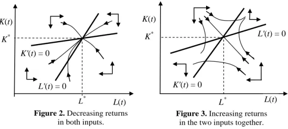
Case 1: 0<α, β<1. In this case both inputs obey decreasing returns to scale. Both demarcation lines are then upward sloping in coordinates (L,K), and the corresponding phase diagrams are in figures 2 and 3. The equilibrium state L'(t)= K'(t)=0_{is a sink in figure 2}(α+β<1) and a saddle in figure 3 Figure 2 displays a dynamic extension for the neoclassical theory. Figure 3, on the other hand, shows that permanent growth in the use of the inputs (and also in q through the production function) is possible when the two inputs together obey increasing returns. If the initial values are great enough, permanent growth takes place while small lead to the collapse of the firm. The profit of a growing firm will increase with time.

). 1

> β

0

(α+

0,K L

0 0,K L

K(t)

K*

K'(t) = 0

L'(t) = 0

L(t) L*

L

* K(t)

K*

K'(t) = 0

L'(t) = 0

L(t)

Figure 2. Decreasing returns in both inputs.

Figure 3. Increasing returns in the two inputs together.

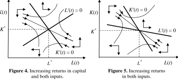
Case 2: α<1, β>1. Here labor obeys decreasing and capital increasing returns to scale. Line L'(t)=0 is now upward and line K'(t)=0 down-ward sloping in coordinates The equilibrium is a saddle (Fig. 4). Permanent growth is possible if the initial values are great enough while low values for lead to the collapse of the firm. Only firms with great enough can survive and their profitability increases with time.

). ,K (L

0 0,K L

0 K

Case 3: α,β>1. Here capital and labor both obey increasing returns to scale Both demarcation lines are now downward sloping in coordinates

). ,

(L K The only possible phase diagram is in figure 5 because the case line 0

) ( ' t =

(17)

enough while low values for lead to the collapse of the firm. If are great enough, the firm grows permanently and increases its profitability with time.

0 0,K L

L(t)

K'(t) = 0

L* L(t)

L'(t) = 0

K(t)

K* L'(t) = 0

K(t)

K*

K'(t) = 0

L*

Figure 4. Increasing returns in capital and both inputs.

Figure 5. Increasing returns in both inputs.

We omitted the case α>1,β<1 because it is symmetric to that in Case 2. In figures 2-5, changes in exogenous variables move the positions of the demarcation lines. If the initial state of the system is the equilibrium, a move in one demarcation line starts an adjustment toward the new equilibrium state in figure 2 and away from the new equilibrium in figures 3-5, unless the initial point happens to be on a saddle-path.

τ

, , ,w₁ r P

7. Increasing Returns to Scale in Human Capital

Next we omit physical capital and concentrate on the role of human capital in the production process. The production function of the firm is assumed as: , ) ( ) ( ) ( 0 α ⎟⎟ ⎠ ⎞ ⎜⎜ ⎝ ⎛ = L t L t BH t q γ ⎟⎟ ⎠ ⎞ ⎜⎜ ⎝ ⎛ = 0 ) ( ) ( R t R D t H

where L(h/ y) is the labor input as earlier, R(h/ y) unit B(

the labor input in the

production of human capital H($/y), and are

positive constants. Notice that H is the flow – and not the level – of human capital, and only increases in human capital are assumed to affect q.

(18)

Human capital is measured by its monetary value when sold to other firms. The profit function is then:

)], ( ) ( )[ 1 ( ) ( ) ( )

( ₁ ₂

0 0 t R w t L w L t L R t R PA

t _⎟⎟ − +τ +

⎠ ⎞ ⎜⎜ ⎝ ⎛ ⎟⎟ ⎠ ⎞ ⎜⎜ ⎝ ⎛ = Π α γ

A= BD.

This model is identical as in the previous section when is replaced by

R

γ

,

K by β, and (1+τ)w₂ by r. Again, either of the two types of labor may obey increasing returns to scale, or they may together cause increasing returns to scale in the production. We could have added in this analysis physical capital, too, and get results where every combination of the three inputs may cause increasing returns to scale in the production. Other forms for the production function could also have been assumed with similar results.

The theories of Lucas (1988) and Romer (1990) base on increasing returns to scale in production due to human capital. However, our mode-ling shows that the somewhat unclear concept of human capital is not a necessity for economic growth. Similar results are obtained with increasing returns for any input, or because several inputs together obey increasing returns. The block diagram in figure 1 gives a hint of how a more detailed description of the production process could reveal elements where effi-ciency can be increased.

8. Conclusions

(19)

In real life there exist factors that slow down and eventually stop the growth of a firm, like increasing wage level, the saturation of the market, the appearance of competing firms, etc. However, we have evidence of long-lasting growth of corporations like IBM, HP, Nokia etc. Even though these growth processes may not last forever, we believe that it is more meaningful to model these as explosive processes rather than to assume that these firms have been approaching their equilibrium states last 20 years, as the neoclassical theory claims. We believe that there are elements in the production processes of these firms that allow them to grow in a profitable way, which elements we modeled here. However, because firms' production methods change with time, one specific model may not keep its accuracy too long.

Appendix

Part A: Continuous time interest rate r(1/y) is defined as the growth rate of invested money x(t)($):

) ( ) ( ' t x t x

r = _x'(_t)=_rx(_t)⇒_x(_t)= _x(_t₀)er×(t−t0).

The unit $/y of x'(t), where y is a time unit, explains that of .r The last equation is the solution of the differential equation with fixed .r With the interest factor is where time t has unit y. The exponent of e is thus dimensionless.

, 0

0 =

t ert

Part B: The necessary conditions for the critical point ∂Π/∂L = 0

/∂ =

Π ∂

= K to maximize the profit are:

, 0 ) 1 ( ₁ 0 1 0 0 = τ + − ⎟⎟ ⎠ ⎞ ⎜⎜ ⎝ ⎛ ⎟⎟ ⎠ ⎞ ⎜⎜ ⎝ ⎛ α = ∂ Π

∂ α− β

w K K L L L AP L . 0 1 0 0 = − ⎟⎟ ⎠ ⎞ ⎜⎜ ⎝ ⎛ ⎟⎟ ⎠ ⎞ ⎜⎜ ⎝ ⎛ β = ∂ Π

∂ α β−

r K K L L K AP K

The sufficient condition for profit maximization is that the first minor determinant of the Hessian matrix is negative, and the second is positive. The Hessian matrix is:

(20)

The first minor of H is and the second minor equals the determinant of the Hessian |H| is:

, / 2

2

1 L

H =∂ Π ∂

, | | 2 2 2 2 2 2 ⎟ ⎠ ⎞ ⎜ ⎝ ⎛ ∂ ∂∂ Π − ∂ Π ∂ ∂ Π ∂ = K L K L H were: , ) 1 ( 2 0 0 2 0 2

2 β α−

⎟⎟ ⎠ ⎞ ⎜⎜ ⎝ ⎛ ⎟⎟ ⎠ ⎞ ⎜⎜ ⎝ ⎛ − α α = ∂ Π ∂ L L K K L AP L , ) 1 ( 0 2 0 2 0 2

2 β− α

⎟⎟ ⎠ ⎞ ⎜⎜ ⎝ ⎛ ⎟⎟ ⎠ ⎞ ⎜⎜ ⎝ ⎛ − β β = ∂ Π ∂ L L K K K AP K and: . 1 0 1 0 0 0

2 β− α−

⎟⎟ ⎠ ⎞ ⎜⎜ ⎝ ⎛ ⎟⎟ ⎠ ⎞ ⎜⎜ ⎝ ⎛ αβ = ∂ ∂ Π ∂ L L K K K L AP L K

Thus: | | [( 1)( 1) ].

) 1 ( 2 0 ) 1 ( 2 0 2 0 2 0 2 2 αβ − − β − α ⎟⎟ ⎠ ⎞ ⎜⎜ ⎝ ⎛ ⎟⎟ ⎠ ⎞ ⎜⎜ ⎝ ⎛ αβ = − β − α K K L L K L A P H

If 0<α<1 then H <0. On the other hand, requirement |H |> 0 corresponds to α+β<1. Thus for the critical point to be a maximum – as is assumed in the neoclassical framework – neither of the two inputs separately or together can obey increasing returns to scale. The stability of the system, too, depends on the Hessian matrix, see for example McCafferty (1990 p. 138). The trace of the Hessian matrix is:

⎟ ⎠ ⎞ ⎜

⎝

⎛α α− ₊β β− ⎟⎟ ⎠ ⎞ ⎜⎜ ⎝ ⎛ ⎟⎟ ⎠ ⎞ ⎜⎜ ⎝ ⎛ = ∂ Π ∂ + ∂ Π ∂ = β α 2 2 0 0 2 2 2 2 ) 1 ( ) 1 ( ) ( ) ( ) ( K L K t K L t L AP K L H Tr .

The system is stable if |H|>0 (α−1)(β−1)>αβ i.e. and 1 < β + α , 0 ) (H <

Tr which occurs certainly if 0<α,β<1; see (Fig. 2).

R E F E R E N C E S

[1] Arrow, K. J., Hahn, F. H. (1971), General Competitive Analysis, San Francisco, California Holden-Day, Inc.

(21)

[3] Chiang, A. C. (1992), Elements of Dynamic Optimization, McGraw-Hill, New-York. [4] De Jong, F. (1967), Dimensional Analysis for Economists, Amsterdam,

North-Holland.

[5] Dixit, A. K. & R. S. Pindyck (1994), Investment Under Uncertainty, New Jersey, Princeton University Press.

[6] Estola, M. (2001), A Dynamic Theory of a Firm: An Application of `Economic Forces', Advances in Complex Systems, Vol. 1, No. 1, 163-176.

[7] Fisher, F. M. (1983), Disequilibrium Foundations of Equilibrium Economics,

Cambridge University Press.

[8] Lucas, R. E. Jr. (1988), On the Mechanics of Economic Development, Journal of Monetary Economics, 22.

[9] McCafferty, S. (1990), Macroeconomic Theory, Harper & Row, Publishers, New York.

[10] Marshall, S. A. (1978), Introduction to Control Theory, MacMillan Press LTD. [11] Mas-Colell, A., M. D. Whinston & J. R. Green (1995), Microeconomic Theory,

Oxford University Press.

[12] Mirowski, P. (1989a), The Rise and Fall of the Concept of Equilibrium in Econo-mic Analysis, Recherches Economiques du Louvain,Vol. 55:4.

[13] Mirowski, P. (1989b), More Heat than Light, Economics as Social Physics, Physics as Nature's Economics, Cambridge University Press.

[14] Ogata, K. (1997). Modern Control Engineering, Third Edition. Prentice-Hall, International (UK) Limited, London.

[15] Romer, P. M. (1990), Endogenous Technological Change, Journal of Political Economy,October 98, 71-102.

[16] Samuelson, P. A. (1942), The stability of equilibrium, Econometrica, Vol. 10, 1-25. In: The Collected Scientific Papers of Paul A. Samuelson, Volume I, ed. by Joseph E. Stiglitz, (1966), Cambridge Mass, M.I.T. Press.

[17] Solow, R. M. (1956), A Contribution to the Theory of Economic Growth. Quarterly

Journal of Economics,Vol. 70, 65-94.

[18] Weiss, C. (1993), Price inertia and market structure: Empirical evidence from Austrian manufacturing, Applied Economics,Vol. 25, 1175-1186.

(22)

ABOUT DISTRIBUTION OF MONEY

IN A FREE MARKET ECONOMY

Karl E. KÜRTEN* and F. V. KUSMARTSEV**1

Abstract. We study a sophisticated model of a market belonging to the class

suggested originally by Angle et al (see Review [1] and references therein) where a fixed number of trading agents exchange and transfer money. We show that the probability distribution of money, income or wealth resulting in the long-term trading process may take a specific form depending on the amount of money rotated in a single turnover process, where all agents are involved. These distributions are associated with a stable steady state of the macroscopic dynamical trading processes and may describe different market economies. The structure of these distributions depends crucially on average income, democracy, the standard of life and other features associated with political and economic structures of the market economy at equilibrium and may be described by a few parameters, only. One of these parameters can be called a temperature, which is similar to one introduced earlier by Yakovenko and collaborators [2,3] and connected with an average money which economic agents have. Such parameter may separate hot and cold markets which behaviour is different. Specifically for some “cold” market economies when the temperature is smaller than average amount of money per agent we find the Boltzmann distribution found before by Yakovenko et al [2,3]. In such market there is a large amount of goods flow and money and the market is associated with countries having a population with high average income and standard of life. However for hotter countries when the temperature tends to the average amont of money per agent this distribution is changing and may take both a Poisson form which gradually transformed from conventional Boltzmann form, when the level of life increases. On the other hand for very cool countries, when the temperature is significantly smaller than average amount of money per agent there arises another form of the money distribution – a Bose-Einstein one [4]. That may arise for very cold market economies, when the most of money are accumulated only in a few economic agents. It is associated normally with not well developed countries having lower level of life, when only a small amount of money and goods flow taken part in the trading processes or in cases when financial crises arises.

Keywords: Market economy, Bose-Einstein distribution, average income,

gamme distributions, gamble trading.

1* Faculty of Physics, Vienna University, 5, Boltzmanngasse, A-1090 Vienna, Austria.

(23)

1. Introduction

We are all now witnesses of the present huge financial crisis started in 2007 and at the present in culmination stage. The crisis has been triggered by a liquidity crisis and next collapses of large financial institu-tions in the United States banking system and around the world. The immediate bailout of banks by national governments was an attempt to save the situation however the downturns in stock markets around the world and the housing market suffered by a far large dip than expected, resulted in numerous evictions and foreclosures. In summary the financial crisis of 2007-2010 started with the US subprime mortgage crisis and still experts are placing different weights upon particular causes of the crisis. The complexity and interdependence of many of the causes, as well as competing political, economic and organisational interests, have resulted in a variety of point of views describing the origin of the crisis. One of the issue discussed is the high corporate and consumer debt levels. The latter cause of the crisis is related to a distribution of money in society and especially related to a part of the population which have a large or medium debt. In the present paper we discuss a simple network model of the market economy with a fixed amount of rotated money and a fixed number of trading agents, who are selling and buying some goods and therewith paying or exchanging money. The flow of the goods is not taken into account, and the focus within this model is on the distribution of the money, which arises in the course of long trading processes. In other words, we are interested in the question: “What is the shape of the money distribution in the equilibrium state in the long term limit of the free market economy?”. Such distribution has been recently studied and compared with existing experimental data [2,3]. This finding has attracted attention of a broad scientific community. In turn that stimulated to reconsider main concepts, which are underlining modern financial econometrics.

2. Model

(24)

random [1]. The total amount of money on a market is fixed and equal to M. We assume that, when two partners are connected they are trading according to some trading law specified by the interaction given below. In the first instance we consider the simplest case when the update rule for the network is stochastic and the network connectivity is annealed (that is at each time step of the time evolution the randomly chosen agent picks a new partner at random).

Initially all agents are given a certain amount of money drawn from an arbitrary probability distribution p(t=0). This initial state is not nece-ssarily taken from a uniform probability distribution used in previous works [2,3]. At each time step a randomly chosen agent acts as a buyer, while the connected randomly chosen agent

i

j acts as the seller. We assume that the amount of the transaction is proportional to the actual funds of the buyer agent which is a plausible assumption. As the result the wealth of the i-th agent decreases as:

i ), ( ) ( = 1)

(t m t pm t

mi + i − i (1)

while for the j-th agent the money increases as: .) ( ) ( = 1)

(t m t pm t

m_j + _j + _i (2)

The model we propose here is reminiscent of Angle's model [1] who introduced two classes of sellers specified by the probabilities and representing different attitudes with respect to buying and selling. In other words the whole population has been divided a priori into two classes with

and being inversely proportional to their educational level, that is and are small or large.

i

p p_j,

i

p

i

p p_j

j

p

First we would like to consider two limiting cases, which allows to obtain exact mathematical results. The first case is when the probability of the money exchange vanishes (p=0). In this case the original distribution of money remains which is m_i(t+1)=m_i(t) for all In the second case each buying agent is spending all his money in each transaction . i ). 1 =

(p As the result he is loosing all his money and after that is expelled from the next trading processes, i.e. from the market. That is after the first time step. At the same time each seller is gaining that is

0 = 1) + t ( m_i = 1) (t+

(25)

except one vanish and all the money will be in the hand of this one single agent.

The time evolution of the models seems to relax towards an equili-brium probability density distribution specified by the gamma distribution:

, )

(

) ( =

) (

1

k x exp x

x P

k k

Γ

β − β −

γ (3)

where the parameter k specifies the shape, while inverse β defines the scale and the tail, respectively. The parameters of the gamma distribution depend strongly on the rate of the money exchange, that is on the value of the parameter p or on the topological structure of the financial trading network. We note that our trading network is equivalent to a gas of

D-dimensional particles [5]. Effectively, the parameter may be related to the number of degrees of freedom of the particles of this D-dimensional gas system. In this analogy each trading agent represents a particle. Then the trading processes of the economic agents are equivalent to the exchanging energy of the gas particles which occurs in mutual collisions. In this analogy the parameter where is the dimension of the space where the gas exists. Then the pre-exponential factor of this gamma distribution may be related to a density of states for this D-dimensional gas. The usage of this analogy may indicate that the parameter

k

, /2 = D

k D

k is proportional to the number of the degrees of freedom of an average economic agent, that is the space dimension .D Here the average is

, = / = >

<m k β kT where we call the parameter T as a temperature of the market. The variance is σ2 =kT/β. For k >1 the distribution has a maximum at x_max =(k −1)T and for large values of k the Gamma distri-bution converges to a Gaussian distridistri-bution with the same moments. For

1 =

k we have the exponential distribution:

.) ( = )

(x exp x

P_γ β −β (4)

3. Numerical Experiments and Simulations

of the market as long term trading

Now let us consider a more general situation, when the value is small. This means effectively that all agents spend only a small fraction of the capital they have. That is they are very cautious not to spend too much.

(26)

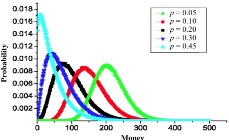
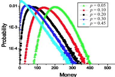
As a result of such trading the distribution of money is taking the bell shaped gamma distribution form (see figure 1).

p= 0.05

p = 0.10

p = 0.20

p = 0.30

p = 0.45

ney

P

robab

ili

ty

Mo

Figure 1. The stationary distribution of money created in a result of the long-term evolution of a free market. The market is characterised by the parameter p, which is associated with the effective fraction of the money of economic agent which he uses in a single trading process. Here we have presented cases when p=0.05, 0.10, 0.20, 0.30, 0.45.

At the value p=0.05 the money distribution is described by the bell shaped gamma distribution form (see, the green line) with parameters

21.3 =

k and β=0.1. The position of the peak of the curve corresponds to ,

/N

M i.e. the money average over all agents, while the area under the curve corresponds to the normalised total amount of money circulating on the market. Such a distribution implies that the majority of agents have roughly the same amount of money about M/N. The fluctuations descri-bing the money exchange of the trading agents around the average are defined by the half-width Γ= 2ln2σ which corresponds here to money units. It is naturally to ask the question: “what is the origin of such a nearly Gaussian distribution of money”? The mean of the distribution corresponds to the value

54

. = / =

> k kT m

(27)

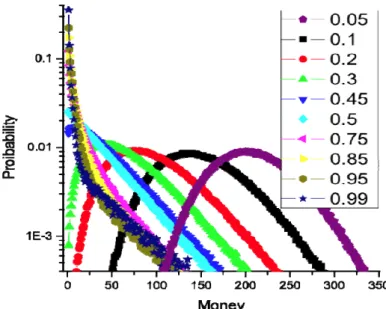
clearly seen when the probability is represented in the logarithmic scale (see figure 2).

p= 0.05

p = 0.10

p = 0.20

p = 0.30

p = 0.45

Figure 2. The distribution of money associated with low values of p (when

p = 0.05, 0.10, 0.20, 0.30, 0.45) in logarithmic scale. The lowest values correspond to Gaussian-like form while large values correspond to more dominant, exponential, Boltzmann distribution. In such a scale one may see clearly the Boltzmann distribution when p = 0.45, which has a gaussian part or a parabolic part just near the maximum only at very small amount of money, m <20.

The exponential tail of the gamma distribution corresponds to the linear part of the curve in this figure, while the central part near the maximum corresponds to a parabolic type curve. One may notice from figure 2 that when the parameter p increases the parabolic curves describing the maximum associated with different p values become more asymmetric. This asymmetry goes together with the creation of a larger high-money exponential tail. The larger the value p the longer the exponential tail and the narrower the bell shaped parabolic part of the gamma distribution associated with the maximum of this distribution. In fact for the only exponential tail remains while the parabolic part and the maximum vanishes (see, the light blue curve presented in figure 3).

1/2 =

(28)

Figure 3. The evolution of the distribution of money when the parameter p

changes. Each separate curve corresponds to a distribution associated with a fixed value of the parameter p. Here we present the distributions for

p = 0.05, 0.10, 0.20, 0.30, 0.45, 0.5, 0.75, 0.85, 0.95 and p = 0.99 values. In the logarithmic scale one may clearly see the changes of the distribution from gaussian-like having a clear maximum at m >0to exponential or Boltzmann type. Finally at large values of p and small money there arises a change in the distribution form especially this concerns to the low money region. That is when the distribution takes the form of Bose-Einstien distribution.

1/2 >

p

(29)

have introduced the temperature of the market with the meaning as an average amount of money per an agent. Such a discovery has created an intensive interdisciplinary discussion between physicists and economists on the question what is an origin of such an distribution in real life, where the total amount of money may not be conserved. Recently it was also shown that such a Boltzmann distribution corresponds to the most optimal configuration of the market where the money are distributed between a fixed numberN of economic agents [4]. Since this exponential tail corres-ponds to the high-money region of the distribution. According to an analogy with the Boltzmann distribution one may state that this part may characterise the most optimal and realistic equilibrium part of the money distribution. However, we still have to answer the question why with increasing values of that is for more gambling economies, the gaussian-like form of the gamma distribution is gradually replaced by the exponential one.

,

p

Thus, numerical simulations show that for 0< p<0.5 there arises an asymmetric Gaussian-like distribution of money with skewness

This distribution is well fitted by the gamma distribution and that has a deep physical sense, because the trading equilibrium network corresponds to a gas of D-dimensional particles. For

. 2/_k1/2

2 / 1 =

p the distribution trans-forms into a pure exponential (see, the table 1, where the parameter k =1, while the gas has the dimension This limit can be explained by symmetry arguments. In short, here each agent spends exactly half of his money during each transaction. For different values of the parameter

). 2 =

D

p the results (the values of the parameters for the resulting gamma distribution) are presented in the table 1:

Table 1

The parameters of the gamma distribution of a network of trading agents.

p k β 0.05 21.3 0.1

0.10 9.58 0.063 0.20 4. 0.0354 0.30 2.32 0.033 0.40 1.45 0.029 0.45 1.2 0.0285

0.50 1. 0.028

(30)

As it can see from table 1 the parameter p corresponds to a fraction of money which a buyer is spending in each transaction. The parameter

β =1/T defines the inverse scale of the distribution function and is equivalent to the inverse temperature of the gas or of the market, T. The parameter corresponds to a dimension of a gas which can be put in a correspondence to this trading network, where the money plays a role of the energy of the gas particles.

k

We observe that when the parameter increases from zero number of the degrees of freedom of the D-dimensional gas or its spacial dimen-sion decreases very fast from and are equal to for the value

On the other hand the scale factor

p

40 =

D D=2

. 1/2 =

p β roughly triples.

4. Bose-Einstein distributions

However when the value p increases and becomes larger than there arises another transformation of the Boltzmann distribution: the exponential distribution is replaced by a Bose-Einstein one. The expo-nential tail is associated with the linear curve presented on the figure 3. This behaviour exists when the money values belongs to the interval while for values of we see that there arises a power law. This separation between these two types of different behaviour becomes more pronounced, when the value

1/2 =

c

p

, 200 < <

30 m m<30

p approaches 1. However in the majority of the region when the money distribution can be described by the following universal fitting formula, known as Bose-Einstein distribution:

1 < < 1/2 p

. 1 exp

= )

( 0

− ⎟ ⎠ ⎞ ⎜

⎝ ⎛ −μ

T m

n x

P_BE (5)

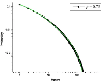
To give an example, for the value the money distribution is presented in the figure 4 in logarithmic scales on both coordinates. The model calculations are presented by triangular points, while the fitting curve is presented by continuous green line.

0.75 =

(31)

p = 0.75

Figure 4. Fit of the money distribution for the parameter with the Bose-Einstein distribution. The value of the chemical potential has been taken equal

to with temperature and normalization constant 0.75

=

p

0

n

1.58 =−

μ T =53 =0.006.

Note that the absolute value of the chemical potential in the fitting curve is significantly smaller than the effective temperature

1.58 =− μ

. 53 =

T In general, for p>0.5 the distribution can be well approximated by the Bose-Einstein distribution (Eq. (5)).

■ p = 0.99

Figure 5. The distribution of money associated with the value p = 0.99 in logarithmic scale. One may see that at large values it is a straight line, i.e. the exponential or the Boltzmann distribution, while at small money region it has a different behaviour. The total distribution can be fitted to Bose-Einstein distribution form (see, eq. (5)).

(32)

. 2 =

D The parameter will correspond to a normalisation factor. In this analogy the parameter will correspond to the chemical potential of these bosons. The values of all these parameters depend on the parameter which control the transferred money fractions.

0

n

μ

,

p

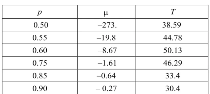
Table 2

p μ T

0.50 –273. 38.59

0.55 –19.8 44.78

0.60 –8.67 50.13

0.75 –1.61 46.29

0.85 –0.64 33.4

0.90 – 0.27 30.4

Table 2: The parameters of the Bose-Einstein distribution of a network of trading agents. For such a distribution the parameter p is corresponding to a fraction of money which each buyer is spending at each transaction. The parameter T corresponds to the temperature of the gas or the market temperature and scales the money distribution, see also the Table 1. The parameter μ corresponds to a chemical potential of a two-dimensional gas which can be put in a correspondence to this trading network, where the money plays a role of the energy. The value of n0 is a normalisation factor.

From table 2 one may see that for the money distribution can be still described by the

0.5 >

p

−

D dimensional gas analogy while the space of the dimensional gas is fixed by D or the whole parameter range of parameter p changes. However when a fraction p of the buyer money rotated in each transaction increases the value of the chemical potential increases and tends to zero. In the tail region we always have a conventional Boltzmann form. For the value

−

D =2 f

> 0.9

(33)

narrow region there is a qualitative crossover of these two Bose-Einstein distributions. Such a Bose-Einstein distribution of money has been recently derived on the basis of statistical mechanics [4], provided that the free economy market is considered as a complex system displaying a chaotic behaviour. Such a distribution may effectively describe a formation of financial crisis as a Bose-Einstein Condensation phenomenon as well as economic growth of human society. In the present case where the Bose-Einstein distribution has been found as a fitting curve these physical arguments may be also applied. From physical point of view the small value of |μ| relative to the value of T means that the system is very close to the possible Bose-Einstein condensation phase transition in this system, which arises when the chemical potential |μ| vanishes exactly. When this happens there arises so-called Bose-Einstein Condensed (BEC) state, where the majority of agents have zero, or have essentially no money. From an economic point of view these “condensed” agents are dead for the market economy. They are in the BEC ground state which is different from the active trading state in which the rest of the agent, do exist. The condensed agents with zero money may be activated by debt, although this may lead to other problem or by a luck when they will sell some product sucessfully. Note, that when the value of the trading parameter reaches 1, the state of the market is exactly in crisis or in the Bose-Einstein Condensed State. There, practically all trading agents except one have no money. This means that they are condensed and form a new form of state known as the Bose-Einstein one.

p

5. Discussion

In the present work we have studied a simple model of the market with a fixed number of economic agents interacting in pairs. Originally before a start of the trading processes all agents have different amounts of money with equal probability. At each time step towards equilibrium the agents form a temporary random network with connectivity

N

. 1 =

k As the result of numerous trading events the probability distribution reaches a state of equilibrium described by the gamma distribution. The financial transactions between agents have been characterised by the parameter p. We studied the time evolution of the money distribution between agents when the parameter p varies between 0 and 1. The small values of p

(34)

which an agent is spending in a trading process. In such a case of the “safe market economy” agents are very cautious to use all their money in a single trading event. While when the agents are “gambling”, that is they to use the largest part of their money in their individual single trading processes. We found that the shape of the money distribution depends drastically on the parameter The total summary shapes of different distributions associated with different values of the parameter

1/2 >

p

.

p

p have been presented in the figure 6. One may see that the safe market economy arising at small values of corresponds to a gamma distribution where the majority of economic agents have approximately the same amount of money (peaked around or very close the average

1/2 <<

p

). /N M

Figure 6. The evolution of the distribution of money when the parameter p

changes in log-log scales. When the value of the spending fraction, p, increases, the shape of money distribution changes dramatically, from Gaussian or Poisson form at very small p to a Bose-Einstein distribution, when p >1/2. When p is close to 1, the distribution is split into two parts of agents having small and large amount of money.

With increasing p the situation gradually becomes worse and there appear more and more poor people. While at values there arises a “gambling” market where the majority of economic agents lost their money. We relate such a state of economic agents with a so-called Bose-Einstein “condensed” state where particles have no energy. In the particular case no money corresponds to no energy in the physical system. Strictly speaking the Bose-Einstein condensed state arises when the value

>

(35)

of the chemical potential, and the number of agents who have no money is of the order of the total number of agents,

0 = μ

.

N However in the present case we do not expect a strict phase transition, which appearance in physical systems depends on many factors such as the space dimensio-nality of the system and others. Therefore we will use these arguments about a formation of a condensed state from economic agents, only qualitatively. We call all agents with no money as being in condensed state, even when the chemical potential values are nonzero, i.e. negative. This is strictly speaking not a condensed state but a pre-course of that state only, since the Bose-Einstein distribution described a normal (non-condensed state) of the system. The (non-condensed state arises when appear more agents with no money than that described by the Bose-Einstein distribution. From figure 6 where the distribution is presented in the log-log scale we see that some agents lost their money at the value

although in such a case the number of zero money agents is still very small (definitely, not a macroscopic number) and still well described in the framework of the Bose-Einstein distribution. We call such an appearance of the zero money agents as the pre-course of the “condensed” state. The number of such pre-course “condensed” agents increases when the value of parameter

, 0.20 =

p

p increases. From figure 6 one may see that already when (the light blue curve) the number of agents in the pre-course con-densed state is a noticeable fraction of the total number of economic agents on the market also still we do not see the Bose-Condensation yet.

1/2 =

p

6. Conclusions

In conclusion, we have considered a simple network model of a free market economy described by the parameter associated with the fraction of money used in individual financial transactions. We have demonstrated that market with gambling trading, i.e. when is very risky and unavoidably leads to a fact that some significant fraction of economic agents will loose their money and condense into a state without money. The next participation of these agents in the market is prohibited unless they will loan the money and receive the debt or be very lucky to sell successfully their property or wealth. On the other hand people get poorer and poorer and most of the people have no money to trade at time period however then suddenly there might arise immense fluctuations when a person without money can trade a wealth and becomes rich again. On average there are few rich people on the market, i.e having a lot of money.

p

1/2 >

p

,

0

(36)

But most of the people remain poor for the long time period observing from one time step to other time step how some people suddenly becomes rich. One can easily avoid such fluctuations by always keeping an amount of savings money which has been done in quite a bit of models, see for example the Ref.

t

[5] and the reference therein. In this case we have also noticed that when the parameter is very close to there arises a forma-tion of two classes which are described by different Bose-Einstein distri-butions. We plan to consider this case and the generalisation of the market with debt in our next publication. On the other hand the market with small values of the parameter

p 1

p that is when the economic agents use a small fraction of their money in the financial operations has a strong tendency to the money equal distribution where all agents have nearly the same amount of money and all agents are active on the market. We believe that this is the model of a stable market.

Acknowledgments

The FVK is grateful to Victor Yakovenko and Lev Bulaevskii for useful discussions and KEK thanks G. Geyrhofer for numerous valuable comments. The work was supported by the Royal Society (London) Inter-national Joint projects 2009/R3, European Science Foundation network-programme, AQDJJ and by EPSRC grant, EP/F005482/1.

REFERENCES

[1] Angle John, Francois Nielsen, and Enrico Scalas, The Macro Model of the Inequality Process and The Surging Relative Frequency of Large Wage Incomes,

pp. 171-196 in A. Chatterjee and B. K. Chakrabarti, (eds.), The Econophysics of Markets and Networks (Proceedings of the Econophys-Kolkata III Conference, March 2007 [http://www.saha.ac.in/cmp/econophys3.cmp/]), Milan: Springer [ISBN: 978-8847006645]. [on-line at: http://arxiv.org/abs/0705.3430]. (2007) and

The statistical signature of pervasive competition on wages and salaries, Journal of Mathematical Sociology. 26, 217-270 (2002).

[2] A. A. Dragulescu and V. M. Yakovenko, The European Physical Journal B, v. 17, pp. 723-729 (2000).

[3] V. M. Yokovenko and I. B. Rosser, Jr., Colloquium: Statistical mechanics of money, wealth, and income, Reviews of Modern Physics 81, 1703 (2009).

[4] F. V. Kusmartsev, unpublished.

(37)

MACROSTATE PARAMETER AND INVESTMENT

RISK DIAGRAMS FOR 2008 AND 2009

Anca GHEORGHIU and Ion SPÂNULESCU*

Abstract. In this paper are made some considerations of the application of phenomenological thermodynamics in risk analysis for the transaction on financial markets, using the concept of economic entropy and the macrostate parameter introduced by us in a previous works [15,16]. The investment risk diagrams for a number of Romanian listed companies in 2008 and 2009 years were calculed. Also, the evolution of the macrostate parameter during financial and economic crisis in Romania are studied.

Keywords: econophysics, stock-exchange markets, entropy, macrostate para-meter, economic crisis.

1. Introduction

During the first decade of 21st_{century a new border science between}

physics and economy, named econophysics, was emerged. At the beginings, econophysics used mostly statistical physics and mathematics methods to characterize and model a range of economic and financial processes, particularly in capital markets, income distribution, interests, and so on (see for example [1-10]).

In the last years, many researchers included in their papers some models based on analogies between the economical phenomena and pheno-mena from other fields of physics such as thermodynamics, electricity, spectroscopy, phase transitions physics, reliability theory and so on [11-16].

In this paper, for the analysis of the risk in the financial market transaction, is appealing to the phenomenological thermodynamics methods and to the statistical physics results concerning statistical interpretation of the entropy and the equilibrium conditions of the physical systems.

In our previous works [15,16] some considerations upon economical information value were made and used in order to introduce a new econophy-sics and technical index for the technical analysis of the stock-market diag-nostic named macrostate parameter. With the help of this defined macrostate

(38)

parameter, the investment risk diagrams for a number of Romanian compa-nies listed at the stock-market in 2006 and 2007 have been established.

In this paper, using the same macrostate parameter and the economic development statistics, the investment risk diagrams for Romanian compa-nies listed in years 2008 and 2009 have been calculed.

2. The Macrostate Parameter

As it was shown in the previous papers [15,16], besides its intrinsic value, characterized by the utility value and trade value, an information type value which determines the denomination, role and importance of any product or service, were considered.

In case when the number of information is large it can be spoken about an information beam with dual aspect, similar to a photon beam or other elementary particles (electrons, protons etc.) characterized by a determined motion mass, impulse, energy etc. [16].

As it was shown in [16] taking into account the above consideration the shares as well as money or economic-financial information about the type volume, or prices of the shares are compared to the particles from an information beam rather by similitude and not by identification with objects from the physical reality. In this case as it was shown in the papers [15,16], for a more complete understanding of the stock evolution from the point of view of the price and transacted volumes, the product

price × transacted volume can be assimilated to the impulse of a particle

(which symbolize the respective financial information) defined by the product pV similar to the impulse p=mv of a particle of mass m and speed v. Such an index can deliver ampler useful information regarding the

“inertia” degree or stability of an asset (shares, financial instruments etc.) than the price, p, or the transacted volume, V, taken separately.

In the like manner, all the information from the financial market can be assimilated with the particles of a gas of impulses p=mv confined in a