COMPUTATION OF MINKOWSKI MEASURES ON 2D AND 3D BINARY IMAGES

COMPUTATION OF MINKOWSKI MEASURES ON 2D AND 3D

BINARY IMAGES

D

L

K

K

M

-F

D

1_{INRA, UR1268 Research Unit on Biopolymers – Interactions and Assemblies, BP 71627, F-44316 Nantes,} 2_{INRA, UR341 Applied Mathematics and Computer Science Unit, F-78352 Jouy-en-Josas}

e-mail: [email protected]

(Accepted June 1, 2007)

ABSTRACT

Minkowski functionals encompass standard geometric parameters such as volume, area, length and the Euler-Poincaré characteristic. Software tools for computing approximations of Minkowski functionals on binary 2D or 3D images are now available based on mathematical methods due to Serra, Lang and Ohser. Minkowski functionals can not be used to describe spatial heterogeneity of structures. This description can be performed by using Minkowski measures, which are local versions of Minkowski functionals. In this paper, we discuss how to extend the computation of Minkowski functionals to the computation of Minkowski measures. Approximations of Minkowski measures are computed using filtering and look-up table transformations. The final result is represented as a grey-level image. Approximation errors are investigated based on numerical examples. Convergence and non convergence of the measure approximations are discussed. The measure of surface area is used to describe spatial heterogeneity of a synthetic structure, and of an image of tomato pericarp.

Keywords: 3D images, Crofton formula, discrete measures, local estimation, Minkowski measures, polyhedral reconstruction.

INTRODUCTION

Standard parameters used in quantitative analysis of spatial structures are the area and the perimeter in 2D, volume, surface area and mean breadth in 3D. Another parameter is the Euler-Poincaré characteristic, related to the topology of the structure. These parameters form the so-called Minkowski functionals. Measuring Minkowski functionals in 2D or 3D digitized images is not a trivial task. For instance, measuring perimeter by counting the number of boundary pixels may be quite inaccurate, see the example shown in Fig. 1. Another common problem is the computation of the number of connected components in a binary image. Results depend heavily on the type of connectivity used. Topological parameters measured on digital images may not fulfil standard relationships and statements holding for continuous case.

The Euler-Poincaré characteristic is a standard connectivity parameter. For a planar structure, it is equal to the number of its connected components minus its number of holes. In 2D digital space, its computation requires the reconstruction of the structure by a set of non-overlapping vertices, edges and polygonal faces. The Euler-Poincaré characteristic of the structure is approximated by the Euler-Poincaré characteristic of its reconstruction. Different types of connectivity may be considered: 4-neighbours,

6-neighbours, 8-neighbours, leading to different approximations of the Euler-Poincaré characteristic. In practice, using the Euler formula the Euler-Poincaré characteristic of this reconstruction can be computed from 2×2 configuration counts (Serra,

1982; Rosenfeld and Kak, 1982).

The Cauchy formula which relates perimeter and number of intercepts provides a simple method for perimeter computation (Serra, 1982). Counting intercepts in 2D binary images is straightforward: it is again a configuration count.

Extensions to 3D images have been derived (see Nagel et al., 2000, Ohser et al., 2002 for the Euler-Poincaré characteristic and Lang et al., 2001 for all other parameters). Again, all needed computations are configuration counts. Methods for computing any parameter belonging to the family of the Minkowski functionals both in 2D and 3D images are now available.

Fig. 1.The digitized disk is the set of pixels contained in the initial disk (represented as black filled circles). A polygonal reconstruction is obtained by joining adjacent pixels of the digitized disk by edges. The perimeter of the disk may be approximated by the total length of the external edges (thick lines). For a disk, this perimeter approximation tends to the perimeter of the square with the same diameter as the digitization grid tends to 0. Hence the relative approximation error is about 25%.

In this paper the methods for computing Minkowski functionals on 2D and 3D images are extended to the computation of Minkowski measures. Concerning the Euler-Poincaré measure, a key argument is Zähle’s definition of Gaussian curvatures for a large class of structures which includes structures with smooth boundaries, as well as polygons and polyhedra (Zähle, 1984; 1986a; 1987). The computation of higher-dimensional Minkowski measures related e.g. to perimeter or surface area is based on the Cauchy and Crofton formulae as for the corresponding Minkowski functionals.

The article is organized as follows. We first recall mathematical definitions of the Minkowski measures. Then the reconstruction of the structure as a complex of convex cells is presented. We develop the computation of Minkowski measures approximations based on this reconstruction, then we present an algorithmic implementation based on configuration counts. The convergence of the Minkowski measures approximations is investigated. Finally, the measure of surface area is used to describe the spatial heterogeneity of a synthetic structure and of a tomato pericarp.

MINKOWSKI MEASURES

DEFINITIONS

LetX be a subset of thed-dimensional Euclidean space Rd (d =1,2,3, . . .) belonging to the class of

unions of sets with positive reach. Finite unions of convex sets, and sets whose boundary is a finite union of twice continuously differentiable manifolds, fall into this class (Zähle, 1984; 1986a).

Such a set is associated with d +1 Minkowski

functionals and measures onRd. Hence a 2D structure

(d = 2) defines 3 Minkowski functionals/measures, while a 3D structure (d = 3) defines 4 Minkowski

functionals/measures. In 2D and 3D, the Minkowski functionals coincide up to known multiplicative constants with standard geometric parameters. Intrinsic volumes are an alternative set of definitions for the same quantities.

For a planar structure X, the first Minkowski functional is the area A of X. The corresponding Minkowski measure is just defined as the restriction to

X of the area (i.e., Lebesgue) measure. If this measure is also denoted by A, then for any planar Borel set

B, A(B) is the area of X∩B and for any real-valued

function φ defined on R2, A(φ) is the integral of φ

onto X. Also note that the total mass of the measure

Ais equal to the area ofX.

The second Minkowski measure is equal toU/2,

where U is the length measure restricted to the boundary∂XofX. HenceU(B)is the length of∂X∩B

andU(φ)is the integral ofφalong∂X. The total mass

ofUis the boundary length ofX.

The third Minkowski measure is equal to πχ, whereχis the Euler-Poincaré measure. The total mass of χ is the Euler-Poincaré characteristic of X. The measure χ is supported by the boundary ∂X. For a planar Borel subsetB:

χ(B) = 1

2π

Z

∂X∩Bκ(x) dx (1)

whereκ(x)refers to the (signed) curvature. Note that the definition above holds if the curvature is defined for all point of the boundary ∂X, e.g. when ∂X is twice continuously differentiable. The general definition of the Euler-Poincaré measure for an arbitrary union of sets with positive reach is given in Zähle (1984).

A spatial structure yields 4 Minkowski measures. LetVbe the volume (i.e., Lebesgue) measure restricted toXand letSbe the surface area measure restricted to the boundary∂X. The measure ¯bis also supported by ∂X. For a Borelian subsetBofR3, ¯b(B)is the integral

over∂X∩Bof the mean curvature divided by 2π. IfX

is convex, the total mass is the so-called mean breadth ofX. Up to an alternative renormalization the measure ¯

fibres. The last measureχ is again the Euler-Poincaré measure:

χ(B) = 1

4π

Z

∂X∩Bg(x) dx (2)

whereg(x) is the Gaussian curvature of∂X atx, i.e.,

the product of the two main curvatures atx.

All measures introduced above are defined over the continuous plane or 3D space. In practice data on structures are most often available as discrete images. Information is available only for a finite subset of points usually organized as a regular grid. We consider here only binary images, a particular case in which information is either true or false. Binary images are usually obtained after a segmentation procedure, i.e., each pixel or voxel is either inside or outside the structure of interest. Our goal is the computation of Minkowski measures based on discrete binary images. This is a non trivial problem for measuresU, S, ¯

b and χ, because their support is restricted to the boundary of the structure. Discrete approximation of curves and surfaces is still an active field of research (Klette and Rosenfeld, 2004). Below we present a

method for computing the measure χ from binary

2D or 3D images. The computation of the other measures is derived both from Euler-Poincaré measure computations and from the Crofton formula.

CROFTON FORMULA

The total perimeter U of a structure can be

expressed by integrating, for all (affine) linesLin the plane, the Euler-Poincaré characteristic of X∩L, the

intersection of the line with the structure:

U=π

Z

χ(L)dL. (3)

where dL is the measure over spatial lines invariant with respect to rigid motion and normalized such that the mass of lines hitting the unit circle equals 2. Note that the Euler-Poincaré characteristic of the one-dimensional subsetX∩Lis just the intercept number

ofX by L. Eq. 3 is known as Cauchy formula. This formula concerns the whole perimeter ofX. However it is easy to see that the formula holds also locally:Ucan be replaced byU(B)in the left-hand side andχ(L)by

χ(B∩L)in the right-hand side. Hence Cauchy formula (Eq. 3) holds also whenU is the perimeter measure instead of the whole perimeter. Then, χ(L) must be considered as the Euler-Poincaré measure associated withX∩L.

The 3D extension of Cauchy formula is called Crofton formula. Special cases of Crofton formula are

S=4

Z

χ(L) dL, (4)

and

¯

b=

Z

χ(P) dP, (5)

where dL is the measure over spatial lines invariant with respect to rigid motion and normalized such that the mass of lines hitting the unit sphere is equal to π and dP is the measure over planes invariant by rigid motion and normalized such that the mass of planes hitting the unit sphere is equal to 2. AgainSand ¯bcan be considered either as total (scalar) parameters or as well as measures.

Hence the measuresU,S and ¯b can be expressed as integrals with respect to lines or planes of Euler-Poincaré measures.

BINARY IMAGES AND DISCRETE

MEASURES

A 2D or 3D binary image can be considered as a subset of a rectangular gridLdwhered=2,3. Such a

grid can be written as

Ld=∆₁Z×. . .×∆_dZ,

where the d-uple (∆1, . . . ,∆d) defines the pixel or

voxel size. A digitization scheme represents how a continuous structureXis digitized into a binary image

Xd. According to the lattice scheme, Xd = X∩Ld.

According to the covering scheme a grid point x

belongs to Xd if the grid cell centered on x hits X. Further details about digitization schemes and so-called digitalizable maps can be found in Serra (1982). Any measure µ on the grid Ld is defined by a

sequence of weightsµ(x),x∈Ldand the relationship µ(B) =

∑

x∈Bµ

(x), B⊂Ld,

i.e.,µ is a weighted sum of Dirac measures. Note that such a discrete measure can be also represented as an image of weights. Below we will see how to compute approximations of the Minkowski measures associated with a continuous structure X from its digitization

Xd. All approximations will be measures on Ld, i.e., images of weights. Hence the computations can be seen as image transforms: Xd 7→ Ad, Xd 7→ Ud etc. whereAd,Ud denote the discrete approximations ofA andU.

Approximations of the planar area measure A

(d = 2) and the volume measure V (d = 3) are

straightforward:

Ad(B) = ∆1∆2#{Xd∩B} (6)

Vd(B) = ∆1∆2∆3#{Xd∩B} B⊂Ld (7) where #{X_d∩B} is the number of pixels or voxels

EULER-POINCARÉ MEASURES

The approximations χd are Euler-Poincaré

measures computed on polygonal and polyhedral reconstructionsX_r.

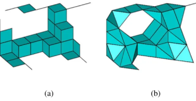
Reconstructions considered here are collections of convex polygonal or polyhedral sets of different dimensions, which touch only by their lower-dimensional faces. Let us call the reconstruction elements cells. For convenience, all lower-dimensional faces of each cell are added to the reconstruction. The cells are chosen such that their vertices belong toXd, and such that their edges belong to a given set of adjacencies (Fig. 2).

The 4-adjacency in 2 dimensions and the 6-adjacency in 3 dimensions, which consider only orthogonal neighbours, lead to cubical reconstruction. Each cell is either a vertex, an edge or a face parallel to the directions of the grid, or a cube corresponding to a tile of the grid. This reconstruction was called cubical complex by Khachanet al.(2000) (Fig. 2).

For 8- and 26-adjacencies, all vertices of the grid with a difference of coordinate at most equal to one for each orthogonal direction are considered as neighbours. In 2D, cells may be triangles and squares. In 3D, cells may be polyhedra with 4 to 8 faces (Fig. 2).

(a) (b)

Fig. 2. Polyhedral reconstructions of a structure

using (a) the 6-adjacency and (b) the 26-adjacency.

The latter reconstruction contains various convex polyhedra, triangular, square and rectangular faces, and diagonal edges.

Other reconstructions may be considered, for example the 6-adjacency in 2 dimensions, the 18-adjacency, or the 14.1 and 14.2-adjacencies which

have been proposed by Ohseret al.(2002).

For a given reconstruction X_r, let us define its envelope Xr as the union of all cells of Xr. The approximation χd is defined as the Euler-Poincaré measure associated withXr.

Note that the Euler-Poincaré measure associated with Xr can not be defined by Eqs. 1 and 2 since the boundary of Xr is not smooth. Instead one can use Zähle’s extension. For polygonal and polyhedral sets the Euler-Poincaré measure is supported by the vertices ofXr. For a vertexxwhereXris convex:

χd(x) =α(X_sr,x)

d , (8)

whereα(Xr,x) is the normal angle ofXr atx, defined as the solid angle of the set of vectors opposite to the tangent cone, and sd is the surface of the unit ball in

dimensiond.

WhenXr is not convex atx, χd(x) depends on the tangent cone ofXratx. It is a matter simple but tedious to show thatχd(x)can be expressed as:

χd(x) =

∑

C∈X_r(x)

(−1)dimCα(C,x)

sd , (9)

where X_r(x₎ is the subset of cells containing x. The measureχd is obtained by:

χd(B) =

∑

x∈Bχd

(x). (10)

It is easy to check that χd(x) equals 1 for an isolated vertex, 1/2 for an edge extremity. In 2D, other

possible values are 1/4 for square corners and 1/8 for

triangle corners when using 8-adjacency on a square grid. In 3D, χd(x) equals 1/8 for the corner of a cube. Using 26-adjacency on a cubic grid leads to 15 different values forχd(x).

By summing χd(x) on all vertices of Xr, one obtains the Euler-Poincaré characteristic of Xr expressed as a double sum on vertices and cells. The summation order can be inverted. As the sum of normalized normal angles of a convex cell equals 1, the total mass of χd can be rewritten as the alternate sum of numbers of vertices (V), edges (E), faces (F) or solids (S) of the reconstruction. We obtain the classical Euler formula:

χd=#V −#E +#F−#S . (11)

LENGTH AND SURFACE AREA MEASURES

Measures of perimeter, surface area and mean breadth require discretization of Crofton formula (Eqs. 3–5). The integrals over lines or planes are approximated by sums over discrete sets of lines or planes.

In the plane, the set of lines can be discretized into horizontal and vertical lines (Fig. 3). An alternative is to use also the 2 diagonal directions. As the density of the lines varies with their direction, they must be weighted accordingly.

Fig. 3. Discrete set of lines. Dots are grid vertices.

Discretization with 2 directions considers only

horizontal and vertical lines (in black). Discretization

with4directions also considers diagonals (in orange).

Line density is higher in the diagonal directions.

For instance, the perimeter expressed as the integral (Eq. 3) is approximated by:

π

n

∑

χ(Lk)

λ(L_k) , (12)

wherek =0, ...,n−1 are indices of the n directions,

andλ(L_k)is the density of the lines parallel to the line

Lk. This density depends on the pixel sizes and may

vary with the line orientation.

Similarly, the set of lines (resp. planes) in the 3D space can be discretized into lines parallel to (resp. planes normal to) the 3 main directions of the grid. Each discrete direction is associated with a weight

ck =1/3, k=1,2,3. A more precise solution is to

use 13 directions, following the (undirected) directions between 2 vertices of the unit cube. Note that this discretization is not isotropic. The choice of Ohser and Mücklich (2000) was used: each direction is represented by a point on the sphere, and weightsck,

k=1, ...,13 are chosen according to the relative area of

the corresponding spherical Voronoi cell, normalized such that ∑ck =1 (Fig. 4). Note that line and plane

densities vary with the direction.

(a) (b)

Fig. 4. Partition of the unit sphere into 6 areas (a), and 26 areas (b), corresponding to the directions of the 6 or 26 neighbours of the central voxel. The areas of the spherical sectors are the same in the case of 6-neighbourhood.

The full discretization of Crofton formula requires the computation of the Euler-Poincaré measure restricted to lines or planes. Let us consider the first approximation (Eq. 12) for the perimeter. For each direction k, let X_r,k be the one-dimensional reconstruction ofX∩Lk. This reconstruction consists

of vertices of Xd∩Lk and edges joining neighbour

vertices. The measures χ(L_k) are approximated by

the Euler-Poincaré measures χd,k associated with the

envelopsXr,k. The final approximation of the perimeter

measure can be written:

Ud(x) = π_n

∑

k

1

λ(L_k)_C∈X

∑

(−1)dimCα(C,x)

2π ,

(13) where λ(Lk) is the distance between two pixels on a

discrete line oriented in the k-th direction. The final approximations for the surface area measure and the mean breadth measure in 3D are given by:

Sd(x) =4

∑

k

ck

λ(L_k)_C∈X

∑

(−1)dimCα(C,x)

4π , (14)

¯

bd(x) =

∑

k

ck

a(P_k)_C∈X

∑

(−1)dimCα(C,x)

4π , (15)

whereλ(L_k)is the density of lines in thek-th direction,

i.e., 1/λ(L_k)is the area of a tile of the lattice formed by

the intersection of the lines with a plane perpendicular to them. The term a(Pk) corresponds to the density

of planes with the k-th direction,i.e., 1/a(P,k)is the

distance between 2 neighbour plates. The coefficients

ck are the weights given to each direction, and are

the unit sphere, with germs depending on the discrete directions (Ohser and Mücklich, 2000).

Note that for approximations of perimeter and surface area measures, there is a choice on the number of directions to use. For the mean breadth measure, one must choose the number of plane directions and the adjacency type for each plane.

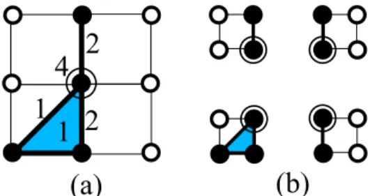
ALGORITHMIC IMPLEMENTATION The Minkowski measure approximations can be computed from the global reconstructionsX_rorX_r,k. For large images, the reconstruction of the entire set, and the computation of normal angles for each cell, can lead to huge computation time. In practice, for each pixel (resp. voxel) x, the computation of X_r(x₎ in Eq. 9 orX_r,k(x₎in Eqs. 13–15 is based only on the 3×3 (resp. 3×3×3) neighbourhood ofx.

Each 3×3 (resp. 3×3×3) neighbourhood is

decomposed in 2×2 (resp. 2×2×2) tiles. A cell may belong to several tiles. In 2D, a pixel belongs to 4 tiles, an isothetic edge (parallel to one of the main directions of the grid) to 2 tiles, a diagonal edge to 1 tile, and a face to 1 tile (Fig. 5). In 3D, a voxel belongs to 8 tiles, an edge to 1, 2, or 4 tiles, depending on its direction, a face to 1 or 2 tiles, and a solid cell to 1 tile. The contribution of each cell is weighted according to the number of tiles it belongs to.

Fig. 5. (a) 3×3 neighbourhood of a pixel (b) its

decomposition in 4 2×2 tiles. The central pixel

belongs to the 4 tiles. Vertical edges belong to 2

tiles, the diagonal edge belongs to only one tile. The triangular face belongs to only1tile.

Thus, approximations (Eq. 9, Eqs. 13–15) are decomposed as sums of 4 (resp. 8) tile contributions. The whole computation is achieved by linear filtering and look-up table transformations. The objective of the linear filtering is to identify each tile configuration as described in Lang et al. (2001). Tile contributions are computed from the filtered image using 4 (resp. 8) look-up table transformations.

APPROXIMATION ACCURACY

First we provide numerical results about the accuracy of the functional approximations. Then we focus on the convergence of the measure approximations.

In two dimensions, three types of shapes were generated and digitized: disks with radius equal to 40 pixels, rings composed of the difference of two concentric disks with radii 40 and 20 pixels, and rotated squares with side length 30 pixels. The comparison of approximations with exact values is given in Table 1.

Table 1.Differences between exact and approximated values for perimeter of planar shapes: a disk, a ring, a square rotated with0,10...45degrees. Approximations

are computed using2and4directions.

shape U U2

d Ud4

disk 251.33 251.31 251.32

ring 376.99 376.99 377.02

square 0 120.00 94.24 112.66

square 10 − 109.96 120.51

square 20 − 120.95 122.68

square 30 − 127.23 120.82

square 40 − 130.38 115.73

square 45 − 131.95 113.18

For three-dimensional shapes, spheres with constant radius of R = 30 voxels, and cubes with

side length L=30 were used. The discretization of

a torus obtained by rotating a 10-radius disk along a perpendicular 15-radius circle was also considered. Comparison of true values and their approximations is given in Tables 2 and 3. If differences are small in the case of the ball, it can be bigger for cubes or torus. In these cases, the effect of the directions discretization is important. Note that for the considered structures, it is reduced when using 13 directions instead of 3.

Table 2.Differences between exact and approximated values for surface area of 3D shapes: a ball, a cube and a torus. The orientation of the shapes is given by the colatitudeθand the azimutϕ.

shape ϕ θ S S3

d S13d

ball 0 0 5026.5 5024.5 5023.6

cube 0 0 2400.0 1600.0 2160.4

cube 45 0 − 1989.3 2146.8

cube 45 45 − 2489.3 2249.0

torus 0 0 5921.7 5713.3 5895.8

torus 45 0 − 5893.3 5878.2

Table 3.Differences between exact and approximated values for the mean breadth of 3D shapes.

shape ϕ θ _b¯ _b¯3

d b¯13d

ball 0 0 40.0 39.9 39.9

cube 0 0 30.0 20.0 27.2

cube 45 0 − 25.0 27.2

cube 45 45 − 31.3 28.4

torus 0 0 47.1 40.0 46.2

torus 45 0 − 48.0 46.2

torus 45 45 − 48.7 47.0

Results about area and volume measure approximations are already available (see, e.g., Kiêu and Mora 2005; 2006). For a large class of planar structures, the approximation error forAd tends to 0 as fast as(∆1∆2)34. Concerning spatial structures, the

approximation error for Vd tends to zero as fast as

(∆1∆2∆3)23.

The convergence of the Euler-Poincaré

characteristic was established for the 2D case by Serra (1982), and extended to the 3D for different types of adjacencies (Nagel et al., 2000; Ohser et al., 2002; Rataj, 2004).

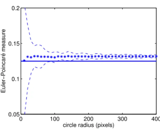
In order to assess the asymptotic behaviour of the Euler-Poincaré measure in 2D, the special case where

X is a disk has been considered. A function ϕ on the plane has been chosen, and the convergence of χd(ϕ) towards χ(ϕ) has been assessed. The chosen functionϕ is a triangle function of θ, defined as the angle between the line joining the origin to x and the horizontal axis. The support of this function is a circular sector, whose axis of symmetry is chosen equal toπ/8 and angular extent toπ/4. This numerical

experiments shows that χd(ϕ) converges as the grid resolution tends to 0 to a value which differs from χ(ϕ)(Fig. 6).

Zähle (1990) provides a criterion which guarantees that Minkowski measures of a reconstruction converge towards the true value. This criterion involves the normals of the reconstruction. For the reconstructions considered in this paper, normals have a limited number of directions, which does not increase with the resolution. The same counter-example can be considered in 3D space. Hence the 3D approximation of the Euler-Poincaré measure does not converge either. More general results on the approximation errors would be of interest.

The mean breadth measure approximation involves approximations of 2D Euler-Poincaré measures. In view of the non-convergence of the latter measure, it is likely that the mean breadth measure approximation does not converge.

0 100 200 300 400

0.05 0.1 0.15 0.2

circle radius (pixels)

Euler−Poincaré measure

Fig. 6. Non-convergence of the 2D Euler-Poincaré

measure approximation. The stars represent χd(ϕ) at

different resolutions computed using the 8-adjacency,

averaged over 100realizations. See the main text for

description of ϕ. The horizontal line shows the true

value of χ(ϕ). The dashed lines show the interval

containing95%of the measurements.

The perimeter measure is concerned with 3 levels of discretization error. At the highest level, the set of line directions is discretized into 2 or 4 directions. Next, the set of lines in given direction is discretized by a series of parallel lines. The line spacing is determined by the grid resolution. At the lowest level, the number of intercepts is approximated by configuration counts. Approximations of the number of intercepts converge as the grid resolution increases. At the intermediate level, the approximation error also converges to zero as the resolution increases. However, the error involved at the highest level does not depend on the spatial resolution. The latter error is expressed as follows:

π

n

n

∑

k=1

Hk, (16)

where Hk denotes the total projection length measure

on a line parallel to the k-th direction. As shown by (Moran , 1966), this errorε is bounded by−0.2146×

U ≤ε ≤0.1107×U for 2 directions and−0.0519×

U≤ε≤0.0262×Ufor 4 directions.

The same types of errors are involved in the surface area measure approximation. By simple calculation the directional errorsεcan be bounded by−0.3333×S≤

ε≤0.1547×Sfor 3 directions and−0.0733×S≤ε≤

GRADIENT PROFILE OF SURFACE

AREA

Many observed structures are not stationary and exhibit heterogeneity. This heterogeneity can be described by the variations of a geometric parameter with the position. Practical solutions often consist in computing the parameter in a subset of the image, defined by a window, and to make the position of the restricted window vary. The use of measures generalizes this principle and overcomes problems such as the choice of the window size, by producing a map of contributions for each pixel or voxel of the image.

The interpretation of Minkowski measures for heterogeneity analysis is not straightforward. Spatial variations at a scale smaller than the size of the objects of interest are not meaningful. Small scale variations can be removed by smoothing. When investigating spatial heterogeneity along a given direction, it is proposed to plot projections of Minkowski measures onto the axis direction. Below, such plots are refered to as gradient profiles.

The interest of gradient profiles in one direction is shown through a synthetic example of spheres with heterogeneous distribution and through the application to a real image of tomato pericarp.

SYNTHETIC STRUCTURE

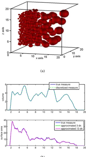
Fig. 7 shows a synthetic ball process presenting a strong heterogeneity. The balls are generated with a density linearly increasing along thex-axis, and by keeping a minimal distance between centroids such that balls do not overlap. The radius of the balls are chosen according to the ball density, such that the volume occupied by the balls remains theoretically constant. The structure is discretized such that the diameter of smaller balls corresponds to 8 pixels.

The approximation of the corresponding surface area measure is computed from the discrete image using 3 and 13 discrete directions. Contributions of voxels with the samex-coordinate are summed in order to produce a profile of surface area. The profiles for the true value and the approximations nicely superimpose. The approximation errors are small and do not disturb the interpretation of the spatial heterogeneity.

(a)

2 4 6 8 10 12 14 16 18 20

0 2 4 6

volume

true measure discretized measure

2 4 6 8 10 12 14 16 18 20

0 10 20 30 40

surface area

true measure approximated 3 dir. approximated 13 dir.

(b)

Fig. 7.(a) An inhomogeneous ball process. The density decreases from left to right, as the typical ball volume increases. A minimal distance between centroids is kept such that the balls do not overlap. (b) The volume and the surface area profiles are estimated along the x-axis and compared with the true measures.

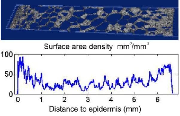
TOMATO PERICARP

The construction of gradient profiles is adapted for describing the changes of morphology in biological structures organized with respect to a reference surface, for example epidermis, organs, or fruits. Tomato pericarp is the fleshy part found around tomato fruit and is made of cells whose morphology varies with depth (Cheniclet, 2005). Quantification of variations of cell morphology is required to study relations with mechnical or sensorial texture properties.

acquired from the external epidermis to the tomato center. After noise filtering, cells were segmented by a 3D watershed operation, resulting into two components: cell interiors and cell walls. Small cells were observed near the epidermises and large cells more or less elongated in the pericarp centre.

Fig. 8. A 3D isosurface representation of a binary image obtained after 3D segmentation of a confocal set of tomato pericarp images. The surface area measure is plotted in the radial direction of the pericarp.

The surface measure of cell walls, and the volume measure of pericarp were computed from the image, and the gradient profile of surface area density was extracted according to the distance to the external epidermis (Fig. 8).

Surface area density is much higher in the region close to the external epidermis, has a lower value in the middle of the pericarp, and increases again near the internal epidermis. As the volume occupied by the cells is nearly constant, and cells are nearly convex, the increase of surface area density can be interpreted as a decrease of cell mean size, and hence as an increase of cell number.

CONCLUSION

In this paper, methods for approximating Minkowski measures of 2D and 3D structures have been developed. These methods are direct extensions of previous works on Minkowski functionals. By using measures, it is possible to compute profiles describing spatial heterogeneity in a given direction.

Convergence results hold for area measure in 2D and volume measure in 3D. Asymptotic error bounds are provided for the perimeter measure in 2D and the surface area measure in 3D. For most practical cases their accuracy seems sufficient when 4 directions

in 2D or 13 directions in 3D are used. Based on numerical counter-examples, it is shown that Euler-Poincaré measure approximations in 2D and 3D, and mean-breadth measure approximations in 3D do not converge.

Further results about the accuracy of these measure approximations are still lacking, making the use of these approximations hazardous. An alternative approach is to consider other types of reconstructions (Klette and Rosenfeld, 2004), whose advantage is that the number of normal directions increases with the spatial resolution.

An implementation of the method for the Matlab software is proposed. The complete functions, as well as some examples, are provided as a library, available on the Internet1_.

REFERENCES

Cheniclet C, Rong WY, Causse M, Frangne, N, Bolling L, Cade J, Renaudin JP (2005). Cell expansion and endoreduplication show a large genetic variablilty in pericarp and contribute strongly to tomato fruit growth. Plant Physiol 139:1984–94.

Klette R, Rosenfeld A (2004). Digital Geometry: Geometric methods for digital picture analysis. Morgan Kaufman Publishers.

Khachan M, Chenin P, Deddi H (2000). Polyhedral representation and adjacency graph in n-dimensional digital images. Comp Vision Image Understanding 79(3):428–41.

Kiêu K, Mora M (2005). Stereological estimation of mean volume: precision of three simple sampling designs. Technical report 2005-1, INRA MIA. Available online. Kiêu K, Mora M (2006). Precision of stereological planar

area predictors. J Microsc 222(3):201–11.

Lang C, Ohser J, Hilfer R (2001). On the analysis of spatial binary images. J Microsc 203(3):303–13.

Moran PAP (1966). Measuring the length of a curve. Biometrika 53:359–64.

Nagel W, Ohser J, Pischang K (2000). An integral geometric approach for the Euler-Poincaré characteristic of spatial images. J Microsc 198:54–62.

Ohser J, Mücklich F (2000). Statistical Analysis of Microstructures in Material Sciences. Chichester: J. Wiley & Sons.

Ohser J, Nagel W, Schladitz K (2002). The Euler number of discretized sets—on the choice of adjacency in homogeneous lattices. Lect Notes Phys 600:275–98. Rataj J (2004). On estimation of the Euler number on thin

slabs. Adv Appl Prob 36:715–24.

Rosenfeld A, Kak AC (1982). Digital picture processing, Vol. 2. Academic Press, second edition.

Serra J (1982). Image Analysis and Mathematical Morphology, Volume 1. Reading: Academic Press. Zähle M (1984). Curvature measures and random sets, I.

Math Nach 119:327–39.

Zähle M (1986a). Curvature measures and random sets, II. Probab Theory Rel 71:37–58.

Zähle M (1986b). Integral and current representation of Federer’s curvature measures. Arch Math 46:557–71. Zähle M (1987). Curvatures and currents for unions of sets

of positive reach. Geom Ded 23:557–67.