Using Alignment Optimization to Test the Measurement Invariance of Gender Role Attitudes in 59 Countries

(1)

Using Alignment Optimization to Test the

Measurement Invariance of Gender Role

Attitudes in 59 Countries

Vera Lomazzi

GESIS - Leibniz Institute for the Social Sciences

Abstract

Several repeated cross-national surveys include measurements of attitudes toward gender roles to investigate individuals’ beliefs regarding the appropriateness of men and women’s roles in a particular context. When used to compare attitudes across countries, these mea-surements reveal critical factors that could cause a lack of equivalence between different cultural contexts, and that could therefore produce misleading results. Nevertheless, the use of such measures to compare country means without assessing measurement equiva-lence is common. It should also be considered that the assessment of equivaequiva-lence within a large-scale sample from cross-sectional surveys through multigroup confirmatory factor analysis (MGCFA) often fails because of the strict requirements necessary.

The current article is used to assess the measurement equivalence of the gender role at-titudes scale included in the last wave of the World Values Survey in 59 countries, with the main goal of identifying the most invariant model for the largest number of groups. The study involved comparing two methods belonging to the frequentist approach: MGCFA and the frequentist alignment procedure, a highly novel and promising method that is still rarely used. Using the first technique, partial scalar invariance was achieved for 27 coun-tries. By employing the frequentist alignment optimization, an acceptable degree of non-invariance was achieved for 35 countries. Thus, the study confirmed the frequentist align-ment procedure as a viable alternative to the MGCFA.

Keywords: Alignment; measurement invariance; measurement equivalence; World Values Survey; gender role attitudes; multigroup confirmatory factor analysis

(2)

Direct correspondence to

Vera Lomazzi, GESIS - Leibniz Institute for the Social Sciences, Cologne, Germany

E-mail: [email protected]

Introduction

Scholars have been well aware of the relevance of the comparative perspective since the dawn of sociology. From Durkheim and Weber onward, the compara-tive approach has been adopted to highlight differences and similarities among dif-ferent groups in an attempt to make theoretical generalizations. This approach is grounded in the basic assumption of comparability; however, are we really compar-ing the same thcompar-ing across the different groups?

In the field of survey research, this concern is intertwined with the issue of measurement equivalence and the methodological approaches used to test for it. According to Horn and McArdle (1992, p. 117), the question of measurement invari-ance is one of “whether or not, under different conditions of observing and study-ing phenomena, measurement operations yield measures of the same attribute.” If measurement invariance is lacking, results can be misinterpreted and conclusions led by “methodological artefacts” (Moors, 2004).

In recent decades, the development of several cross-cultural and repeated sur-vey programs has increased the possibilities for comparative research, both across cultural groups and over time. The efforts made by these programs to guarantee the quality of the data collected lead to the provision of more reliable data, but numerous issues can arise that result in the lack of effective equivalence. In addi-tion to the common causes of non-invariance, such as differences in modes of data collection, sampling, and translation issues (van de Vijver & Tanzer, 2004), cultural biases could arise from the different interpretations of the questions; furthermore, social desirability and acquiescence can also differ by context (Heath, Martin, & Spreckelsen, 2009). The risk of comparing “apples and oranges,” as raised by Steg-mueller (2011), is therefore always in play. The scientific discourse in this field has recently been reinvigorated by two emerging debates, one questioning formative versus reflexive approaches to the study of latent concepts, and the other addressing the exact versus approximate approaches to the concept of equivalence itself, with the consequential development of new techniques to assess invariance.

(3)

that are only applicable for reflective indicators on the same indicators that they claim to be formative, and thus have made their argument less convincing. An example of this can be seen in the paper by Inglehart and Baker (2000) in which the authors aimed to test the postmaterialism theory in 43 societies. They identified 10 items selected from the World Values Survey carried out in 1990–91 and 1995–98 that tap the “Traditional vs. Secular-rational Values” and the “Survival vs. Self-expression Values”, following their combinatory logic. However, to demonstrate that these two dimensions of cross-cultural variations exist both at national and individual levels, they then used a factor model, which is a technique for dealing with reflective indicators.

In addition, as pointed out by van Vlimmeren, Moors, and Gelissen (2016), the formative approach emphasizes the researcher’s point of view; thus, the index could measure the concept as it is framed in the social researcher’s mind, neglecting what is going on in the minds of respondents and the fact that the meaning given to that item, or the way of responding, can be culturally dependent. Welzel’s approach has also been criticized because it underestimates the problem of cross-cultural equivalence and measurement errors (Alemán & Woods, 2015; van Deth, 2014; van Vlimmeren et al., 2016).

Scholars who refer to dimensional logic have strongly argued for the impor-tance of equivalence in comparative studies. Alemán and Woods (2016) widely demonstrated that the postmaterialism and emancipative measures built through the formative approach are not equivalent. In their response, Welzel and Inglehart (2016) expressed the idea that measurement invariance is overrated and is not nec-essary when adopting a combinatory logic; instead, convergence with external cri-teria is sufficient to validate the measure and use it at the aggregate level.

(4)

The present study, which adopted the reflective approach, had a two-fold goal. The first was to assess the measurement invariance of gender role attitudes by iden-tifying the most invariant model across the largest group of countries among those available in the sixth wave of the World Values Survey (WVS). The second was to explore two different methods to assess equivalence, both belonging to the frequen-tist approach; in addition to MGCFA, the new frequenfrequen-tist alignment optimization was also adopted, and the results then compared.

Approaches to Measurement Invariance

Among the methods often employed to assess measurement invariance, including latent class modeling (Kankaraš & Moors, 2009) and item response theory (Mill-sap, 2010), MGCFA has been the most commonly used (Davidov et al., 2015). These methods refer to the traditional approach to measurement invariance, which has its roots in the concept of “exact equivalence.” In other words, the test of gen-eral theories and the comparison between different groups will be successful if the instrument used to compare them is exactly the same.

Previous studies have referred to three levels of measurement invariance: con-figural, metric, and scalar (Steenkamp & Baumgartner, 1998). The first of these refers to the fact that the construct responds to the same configuration in all groups; in other words, the same pattern of factor loading is shown across the groups. Met-ric invariance requires that the unit of measurement is the same, so that the factor loadings are constrained to be equal across the groups. The third level of invariance is the most demanding, as scalar invariance requires equality in factor loadings and indicator intercepts. Comparing covariances and unstandardized regression coeffi-cients across the groups is also possible when metric invariance is reached, but only by achieving scalar invariance can the latent means be compared (Davidov, 2010; Steenkamp & Baumgartner, 1998). However, Byrne et al. (1989) and Steenkamp and Baumgartner (1998) argued that partial invariance is also an acceptable condi-tion for comparing means. In this case, at least two items with equal parameters (factor loadings for partial metric invariance, and factor loading and intercepts for partial scalar invariance) must be identified.

(5)

fulfill. It is often impossible to achieve full invariance since the possible violations in terms of equivalence increase as the number of groups is increased (Davidov, Meuleman, Billiet, & Schmidt, 2008; Davidov, Meuleman, Cieciuch, Schmidt, & Billiet, 2014). Researchers must employ a lengthy procedure to identify an accept-able partially invariant model, which generally requires numerous large modifi-cation indexes; however, these modifimodifi-cations can lead to the risk of producing an inappropriate model because of “the scalar model being far from the true model,” as pointed out by Asparouhov and Muthén (2014, p. 495). Marsh et al. (2017, pp. 10–12) clearly explained this issue, which concerns the problems caused by the stepwise approach that leads to achieving partial invariance. The main argument is that the achievement of a good fit by freeing parameters does not guarantee that means are unbiased. In addition, because of the multicollinearity in the modifica-tion indices, the selecmodifica-tion of the parameters to be freed risks being arbitrary and thus overlooking other potentially better models.

To avoid these risks, another pragmatic solution is to reduce the number of groups compared, but this also reduces the possibility of substantive analyses, with the consequential risks of comparing groups that tend to be culturally more similar and discarding groups that may be of real interest to the scholar.

To express this as well as van de Schoot et al. (2013), researchers find them-selves caught between the two “monsters” of Scylla and Charybdis. Scylla, the six-headed monster, frightens scholars by imposing a model that, to achieve measure-ment invariance, poorly fits the actual data; Charybdis scares them with a model that, while fitting the data, is not invariant. Nowadays, the concept of “approximate equivalence” introduced by Muthén and Asparouhov (2012, 2013), appears to be the most feasible way of navigating between the two mythological monsters.

The two approaches rely on different assumptions. In the exact approach, the differences between factor loadings/intercepts among the groups are zero: they are exactly equal among the groups. In contrast, approximate equivalence considers that loadings/intercepts do not have to be identical among groups that are culturally different. This means that, even if the mean of the loadings/intercepts variations is zero, some slight differences are permitted. The recently developed alignment optimization can be employed in both the approximate/Bayesian and the exact/ frequentist framework. In the latter case, its use could be particularly fitting for those who prefer to stick to the frequentist approach but skip the aforementioned problems caused by the stepwise process employed to achieve partial invariance.

(6)

aims to contribute to the exploration of this new method to assess measurement equivalence.

Alignment Optimization

Developed by Asparouhov and Muthén (2014) as an alternative to MGCFA, this method estimates the factor means without constraining loadings and equal inter-cepts across groups, and it discovers the most optimal measurement invariant pat-tern.

Different from the MGCFA, which assumes measurement invariance, the basic assumption of the alignment is that the number of non-invariant parameters and the degree of non-invariance can be kept to a minimum. This allows for find-ing an invariant pattern across the groups, and for estimatfind-ing factor means and variances while considering the real differences in loadings and intercepts among groups. As a complementary output, the alignment procedure provides elements to assess the degree of non-invariance, which is helpful in evaluating whether to trust and accept the alignment results.

The frequentist alignment optimization technique begins by adopting the max-imum likelihood (ML) method to estimate the configural model, where parameters do not all have to be equal, with factor means fixed at zero and factor variances fixed at one. This is model zero, the best-fitting model possible among the groups included in the analysis, without any restrictions on the parameters. After the opti-mization procedure, which involves applying a simplicity function that essentially works as the rotation criteria for the exploratory factor analysis (Asparouhov & Muthén, 2014, pp. 496–498), the final model retains the same fit as the configural model (model zero) but minimizes the amount of non-invariance.

(7)

The Measurement of Gender Role Attitudes in

Comparative Research

The measurement of gender role attitudes appears to be particularly sensitive to construct bias, which occurs when “the construct measured is not identical across cultural groups” (van de Vijver & Tanzer, 2004, p. 120). In fact, different ways of defining gender roles are established across cultural contexts; institutional factors such as welfare regimes, religious traditions, or labor market dynamics have his-torically contributed to the development of different gender cultures across societ-ies, prescribing gender roles accordingly (André, Gesthuizen, & Scheepers, 2013; Lomazzi, 2017a; Sjöberg, 2004). This is reflected not only in the shaping of gender beliefs, but also in the meaning given to the questions used to investigate these concepts (Braun, 1998, 2009), with the consequential result of a lack of equivalence between different cultural contexts, and therefore misleading results.

Irrespective of such a potential risk, the use of these measurements in compar-ative studies is relcompar-atively widespread. Only recent studies have introduced the eval-uation of the quality of the measurement instruments in this field. Lomazzi (2017b) evaluated the cross-sectional reliability and stability of the configural structure of the gender role attitudes scale employed by the European Values Study across 26 countries, addressing caution in the use of the scale because not enough of it is ten-able. Van Vlimmeren, Moors, and Gelissen (2016) recently analyzed family values and gender role items from the 2008 European Values Study, adopting the perspec-tive of clusters of cultures to address the variation in the meaning given to items and in the way people who belong to different cultures answer the same questions. They clustered countries according to their similarity in covariances between items, and showed that such clusters are internally more invariant and then more comparable. Constantin and Voicu (2014) tested the invariance of the gender role scales included in the 2002 International Social Survey Programme (32 countries) and in the 2005 WVS (45 countries) using MGCFA. Their results showed that scalar invariance was not achieved in either case.

(8)

The Current Study

The aim in the present study was to assess the measurement invariance of the gen-der role attitudes scale employed by the last wave of the WVS, and to explore the limitations and potential of different methods in this assessment.

It has been suggested that the frequentist alignment method is highly conve-nient when analyzing several cultural groups (Kline, 2015; Muthén & Asparouhov, 2014). It also allows for overcoming the problems of the dubious model related to the achievement of partial invariance through MGCFA; therefore, in addition to the traditional MGCFA, its use appeared to be appropriate in the present study. Follow-ing a step-by-step procedure, the frequentist alignment optimization was employed to identify the best invariant model for as many groups as possible.

Methods

Data and Measurements

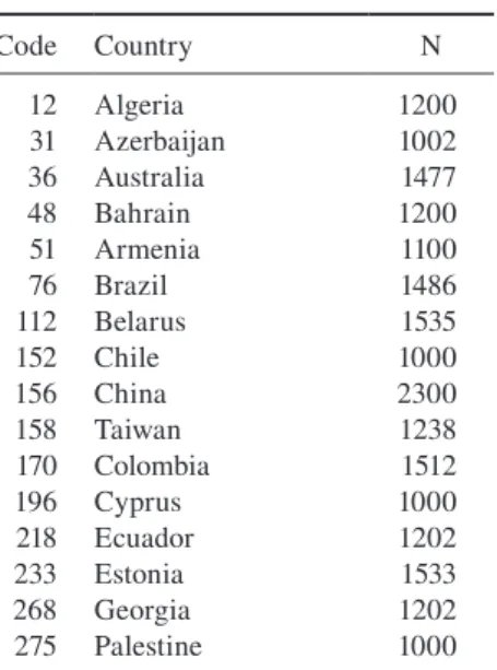
The study considered 59 of the 60 countries investigated by the sixth wave of the WVS (2015), giving a total sample size of 89,320 respondents (Argentina was excluded from the analyses because it had no valid case in one of the measures of interest). Table 1 shows each country’s sample sizes and the country codes later used as references in the alignment output.

Table 1 Reference code and sample size by country

Code Country N

12 Algeria 1200

31 Azerbaijan 1002

36 Australia 1477

48 Bahrain 1200

51 Armenia 1100

76 Brazil 1486

112 Belarus 1535

152 Chile 1000

156 China 2300

158 Taiwan 1238

170 Colombia 1512

196 Cyprus 1000

218 Ecuador 1202

233 Estonia 1533

268 Georgia 1202

(9)

Code Country N

276 Germany 2046

288 Ghana 1552

344 Hong Kong 1000

356 India 5659

368 Iraq 1200

392 Japan 2443

398 Kazakhstan 1500

400 Jordan 1200

410 South Korea 1200

414 Kuwait 1303

417 Kyrgyzstan 1500

422 Lebanon 1200

434 Libya 2131

458 Malaysia 1300

484 Mexico 2000

504 Morocco 1200

528 Netherlands 1902

554 New Zealand 841

566 Nigeria 1759

586 Pakistan 1200

604 Peru 1210

608 Philippines 1200

616 Poland 966

634 Qatar 1060

642 Romania 1503

643 Russia 2500

646 Rwanda 1527

702 Singapore 1972

705 Slovenia 1069

710 South Africa 3531

716 Zimbabwe 1500

724 Spain 1189

752 Sweden 1206

764 Thailand 1200

780 Trinidad and Tobago 999

788 Tunisia 1205

792 Turkey 1605

804 Ukraine 1500

818 Egypt 1523

840 United States 2232

858 Uruguay 1000

860 Uzbekistan 1500

887 Yemen 1000

Total 89320

(10)

Gender role attitudes were measured through a battery of items, formulated as follows: 1) One of my main goals in life has been to make my parents proud (v49); 2) When a mother works for pay, the children suffer (v50); 3) On the whole, men make better political leaders than women (v51); 4) A university education is more important for a boy than for a girl (v52); 5) On the whole, men make better busi-nesses executives than women (v53); and 6) Being a housewife is just as fulfilling as working for pay (v54). Responses to these statements were rated using scores ranging from 1, “Strongly agree,” to 4, “Strongly disagree.”

A preliminary exploratory factor analysis showed that the first item (“One of my main goals in life has been to make my parents proud”) was far from belonging to the same latent concept of the scale (see Table A.1 in the Appendix). This was already imaginable from the content, as it related to feelings toward parents rather than to gender roles. Therefore, this item was not included in further analyses. The other five items were loaded on a unique factor, reflecting only one conceptual dimension.

Analysis Strategy

In order to achieve the two-fold goal of this study, the measurement equivalence was assessed in parallel, initially by performing MGCFA and then by employing the frequentist alignment method. In both cases, the Mplus 7.4 statistical modeling program (www.statmodel.com) was used and the same step-by-step procedure fol-lowed. Finally, the results obtained using the two techniques were discussed.

The criterion that guided the analytical strategy was the idea of finding a bal-ance between the aim of including the biggest number of groups (ideally all those included in the survey) and the need for good enough coverage of the concept “atti-tudes towards gender roles” through the indicators included in the model.

In both procedures, the starting point was therefore the assessment of the 5-item model among all the available groups. Although prioritizing the ambitious aim of comparing as many countries as possible, when this first step did not allow for a reliable means comparison the second step was to identify the item that dis-played the most non-invariant parameters and then exclude it from the ment model. In this way, a 4-item model was identified and, again, the measure-ment equivalence was conducted across all the groups. A 3-item model was also considered, but because of several problems in the model identification, no further analyses were carried out. The strategy then included a third step, which aimed to identify an invariant measurement for a subset of groups.

(11)

achieved, a close investigation of the modification indexes allowed identification of the most non-invariant parameters, which were gradually released to assess par-tial invariance. The measurement invariance was evaluated while considering the recommended cut-off criteria for the change in model fit: ΔCFI <0.01; ΔRMSEA <0.015; ΔSRMR <0.03 (Chen, 2007; Hu & Bentler, 1999). In the third main step, to reach an invariant measurement for a subset of groups, the most “problematic” groups (identified on the basis of the modification indices) were subsequently omit-ted.

Multigroup confirmatory factor analysis and the alignment method employ different computing procedures, which could result in different model fits, model identification, and, consequently, different subsets of groups. To assess the mea-surement equivalence using the frequentist alignment method, the analysis there-fore began again using the original full sample.

The same procedure was applied at each of the three main steps; the align-ment optimization was run using the ML estimator and the output was read to iden-tify the amount of non-invariant parameters. Following the rule of thumb suggested by Muthén and Asparouhov (2014), a Monte Carlo investigation was performed to determine whether population values could be recovered via the alignment.

The Monte Carlo simulation was conducted using the parameters estimated by the alignment procedure as a data-generating population parameter values, defin-ing a hypothetical sample of 1,500 units (the average sample size of the groups included in this study). This was performed both when the non-invariant rate was higher than 25%, as recommended by the developers of the alignment method (Muthén & Asparouhov, 2014), and also when this rate was lower, to validate this limit.

To select the item to be excluded using the measurement model (from step 1 to step 2) and the group to be dropped (from step 2 to step 3), the alignment opti-mization results were used as a diagnostic tool to identify the item (or group) that displayed the highest number of non-invariant parameters.

Results

(12)

MGCFA Results

Table 2 summarizes the results from the first step using the traditional assessment of measurement equivalence of the 5-item model. For 2 of the 59 countries (Nige-ria and Pakistan), the model fit was too poor, and these countries were excluded. The tests therefore refer to 57 countries. By releasing two factor loadings (v54, v52), partial metric invariance could be considered acceptable, even if the change in comparative fit index (CFI) was somewhat borderline (0.014). In order to test for partial scalar invariance, up to three intercepts were progressively released. However, this was not sufficient to establish partial scalar invariance; even if the changes in RMSEA and SRMS fitted the requirements, the change in CFI was higher than 0.01 (0.031). Moreover, the RMSEA value exceeded the cut-off criteria for an adequate fit of 0.08.

Item v54 (“Being a housewife is just as fulfilling as working for pay”) was identified as the most critical and excluded from the measurement model for the second step of the analysis with the 4-item model. The country-by-country model fit assessment provided an acceptable model fit for 57 countries (the model did not fit the data for Pakistan and Egypt). As with the 5-item model, only partial metric invariance was achieved (Table 3) by releasing two factor loadings; on releasing two intercepts, partial scalar invariance was then tested. However, the results were unsatisfactory, taking into consideration all the global fit measures and the change in model fit from the partial metric model (RMSEA 0.106; ΔRMSEA 0.027; ΔCFI 0.034).

In the third step, because the 4-item model showed a better model fit, this model was tested again while subsequently dropping countries. The gradual selec-tion, carried out on the basis of the modification indices, resulted in dropping 32 countries. Table 4 summarizes the MGCFA results for the remaining 27 countries;1

partial metric and partial scalar invariance were achieved by releasing two loadings and two intercepts.

(13)

Table 2 MGCFA results. Global fit measures for the exact measurement equivalence of the 5-item model, 57 countries

Chi2 (dF) RMSEA CFI SRMR

configural 2902.035 (285)*** 0.078 0.964 0.032

metric 7763.249 (509)*** 0.097 0.900 0.090

partial metric 4007.569 (397)*** 0.078 0.950 0.050 partial scalar 6283.398 (453)*** 0.093 0.919 0.063 Note: dF= degrees of Freedom; RMSEA= Root Mean Square Error of Approximation;

CFI= Comparative Fit Index; SRMR= Standardized Root Mean Square Residual; *** p <0.001; ** p <0.01; * 0.01≤ p ≤ 0.1

Table 3 MGCFA results. Global fit measures for the exact measurement

equivalence of the 4-item model, 57 countries

configural 1469.091 (114)*** 0.089 0.979 0.024

metric 3570.189 (282)*** 0.088 0.949 0.073

CFI= Comparative Fit Index; SRMR= Standardized Root Mean Square Residual; *** p <0.001; ** p <0.01; * 0.01≤ p ≤ 0.1

Table 4 MGCFA results. Global fit measures for the exact measurement

equivalence of the 4-item model, 27 countries

configural 575.829 (54)*** 0.084 0.982 0.024

metric 1162.631 (132)*** 0.075 0.964 0.060

(14)

Frequentist Alignment Results

The alignment optimization was initially carried out on the original full set of 59 countries. In this first step of the analysis, the overall non-invariance was 50.8% and the Monte Carlo investigation (results for four groups are displayed in Table A.2 in the Appendix) confirmed the poor recovery of the sample; therefore, the alignment results cannot be used to compare means.

This procedure revealed its diagnostic potential. In addition to identifying the overall amount of non-invariance, we immediately recognize the most (non-)invari-ant parameters. This was the case for item v54 (69 non-invari(non-)invari-ant parameters), from this point not considered for further analysis, which proceeded in the second step with the 4-item model. The degree of non-invariance dropped to 39.0% and the Monte Carlo investigation confirmed that means comparison would not be reliable, as most of the parameter estimates were biased (Table A.2 in the Appendix).

At this point, the alignment results were used as a diagnostic tool to iden-tify the groups presenting the highest number of non-invariant parameters, which were progressively left out. With a reduced sample of 47 countries, the amount of non-invariance was 26.9%. The results of the Monte Carlo investigation (Table A.3 in the Appendix) displayed a poor replication of the factor means. By excluding countries with more than four non-invariant parameters from the analysis, the use of the alignment procedure with 34 countries2_{provided 21.0% of non-invariance}

(Table 5). This result met the recommended rule of thumb and could be considered acceptable. The Monte Carlo simulation was run while expecting results as good as those reported by the previous pioneering studies (Asparouhov & Muthén, 2014; Muthén & Asparouhov, 2014). While this was not always the case for all the groups and parameters, the global recovery in the Monte Carlo investigation improved, particularly for the factor means that were meant to be compared (Table A.3 in the Appendix). Considering the current state of the art, the results from the alignment optimization are acceptable, even if more simulations designed to determine a clear rule of thumb are probably necessary.

(15)

Table 5 Alignment results. Approximate measurement (non) invariance for intercepts and loadings of the 4-item model, 34 countries

Variable Intercept Loadings

V50 31 48 51 (76) (112) 156 170 (268) (288) 368 (398) (400) 410 414 (422) (434) (566) 586 604 608 (616) (634) (642) (643) (716) 752 780 (788) (792) (804) 818 858 (860) (887)

(31) 48 51 76 (112) 156 170 268 288 (368) 398 400 410 (414) 422 434 566 586 604 608 616 634 642 643 716 752 780 788 792 804 (818) 858 860 (887)

V51 31 48 (51) (76) 112 156 (170) 268 288 368 398 400 (410) 414 422 434 566 586 (604) 608 616 (634) (642) 643 716 (752) 780 (788) 792 (804) 818 (858) 860 887

31 (48) 51 76 112 156 170 268 288 368 398 400 410 414 422 434 566 586 604 608 616 (634) 642 643 716 752 780 788 792 804 818 858 (860) 887

V52 31 48 51 76 (112) (156) 170 (268) 288 368 398 400 410 414 422 (434) 566 586 (604) 608 (616) 634 642 643 716 752 780 (788) 792 804 818 858 860 887

31 48 51 76 112 156 (170) 268 288 368 398 400 (410) 414 422 434 (566) 586 (604) (608) 616 634 642 643 716 752 (780) 788 792 804 818 (858) (860) 887 V53 31 48 51 76 112 156 170 268 288 368

398 (400) 410 414 422 434 566 586 604 608 616 (634) 642 643 716 752 780 (788) 792 804 818 858 860 887

31 48 51 76 112 156 170 268 288 368 398 400 410 414 422 434 566 586 604 608 616 634 642 643 716 752 780 788 792 804 818 858 860 887

Note: numbers indicate the country code (see Table 1). The parentheses indicate whether the parameter (intercept or factor loading) is non invariant for that specific group (coun-try code) by variable (v50 to v53).

(16)

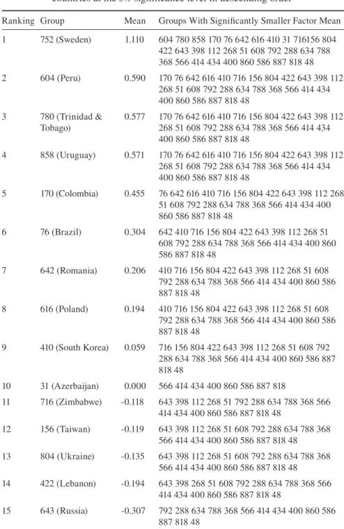
Table 6 Alignment results. 4-item model, factor mean comparison for 34 countries at the 5% significance level in descending order

Ranking Group Mean Groups With Significantly Smaller Factor Mean 1 752 (Sweden) 1.110 604 780 858 170 76 642 616 410 31 716156 804

422 643 398 112 268 51 608 792 288 634 788 368 566 414 434 400 860 586 887 818 48 2 604 (Peru) 0.590 170 76 642 616 410 716 156 804 422 643 398 112

268 51 608 792 288 634 788 368 566 414 434 400 860 586 887 818 48

3 780 (Trinidad &

Tobago) 0.577 170 76 642 616 410 716 156 804 422 643 398 112 268 51 608 792 288 634 788 368 566 414 434 400 860 586 887 818 48

4 858 (Uruguay) 0.571 170 76 642 616 410 716 156 804 422 643 398 112 268 51 608 792 288 634 788 368 566 414 434 400 860 586 887 818 48

5 170 (Colombia) 0.455 76 642 616 410 716 156 804 422 643 398 112 268 51 608 792 288 634 788 368 566 414 434 400 860 586 887 818 48

6 76 (Brazil) 0.304 642 410 716 156 804 422 643 398 112 268 51 608 792 288 634 788 368 566 414 434 400 860 586 887 818 48

7 642 (Romania) 0.206 410 716 156 804 422 643 398 112 268 51 608 792 288 634 788 368 566 414 434 400 860 586 887 818 48

8 616 (Poland) 0.194 410 716 156 804 422 643 398 112 268 51 608 792 288 634 788 368 566 414 434 400 860 586 887 818 48

9 410 (South Korea) 0.059 716 156 804 422 643 398 112 268 51 608 792 288 634 788 368 566 414 434 400 860 586 887 818 48

10 31 (Azerbaijan) 0.000 566 414 434 400 860 586 887 818

11 716 (Zimbabwe) -0.118 643 398 112 268 51 792 288 634 788 368 566 414 434 400 860 586 887 818 48

12 156 (Taiwan) -0.119 643 398 112 268 51 608 792 288 634 788 368 566 414 434 400 860 586 887 818 48 13 804 (Ukraine) -0.135 643 398 112 268 51 608 792 288 634 788 368

566 414 434 400 860 586 887 818 48

14 422 (Lebanon) -0.194 643 398 268 51 608 792 288 634 788 368 566 414 434 400 860 586 887 818 48

(17)

Ranking Group Mean Groups With Significantly Smaller Factor Mean 16 398 (Kazakhstan) -0.318 792 288 634 788 368 566 414 434 400 860 586

887 818 48

17 112 (Belarus) -0.335 792 288 634 788 368 566 414 434 400 860 586 887 818 48

18 268 (Georgia) -0.345 792 288 634 788 368 566 414 434 400 860 586 887 818 48

19 51 (Armenia) -0.369 792 288 634 788 368 566 414 434 400 860 586 887 818 48

20 608 (Philippines) -0.374 788 368 566 414 434 400 860 586 887 818 48 21 792 (Turkey) -0.556 788 368 566 414 434 400 860 586 887 818 48 22 288 (Ghana) -0.573 368 566 414 434 400 860 586 887 818 23 634 (Qatar) -0.655 566 414 434 400 860 586 887 818 24 788 (Tunisia) -0.701 566 414 434 400 860 586 887 818 25 368 (Iraq) -0.801 434 400 860 586 887 818 26 566 (Nigeria) -0.864 434 400 860 586 887 818 27 414 (Kuwait) -0.906 887 818

28 434 (Libya) -1.031 818

29 400 (Jordan) -1.031 818 30 860 (Uzbekistan) -1.036 31 586 (Pakistan) -1.144 32 887 (Yemen) -1.152

33 818 (Egypt) -1.184

34 48 (Bahrain) -1.242

Note: In the last column, groups are indicated by the country code (see Table 1)

(18)

questions and conceptualizing of gender roles? Would adopting a “cluster of cul-tures approach” (van Vlimmeren et al., 2016) provide further insights?

Concluding Remarks

The current study aimed to contribute to the debate concerning measurement invariance by using data from a large-scale cross-national survey to make applica-tive use of the frequentist alignment method. Data related to gender role attitudes, and the assessment was addressed to identify the most invariant model across the largest subset of groups (ideally, all). Adopting a step-by-step procedure, both the methods initially led to a model modification by reducing the measurement from a 5-item model to a 4-item model. The two procedures converged in detecting the item v54 (“Being a housewife is just as fulfilling as working for pay”) as the least invariant. The option of omitting it found additional support in the critical content analysis of Braun (1998), who pointed out that the understanding of this item can be fairly controversial because of the focus on fulfillment and the benefits from two conditions, rather than on gender roles (Braun, 1998, p. 116).

In the final step, an invariant measurement model was identified for a subset of groups. With the MGCFA, partial scalar invariance was achieved for 27 countries, which would allow for a comparison of means among these countries. However, several model modifications were necessary to achieve it.

On the contrary, with the alignment optimization such modifications are not part of the procedure; the final model retains the same fit of the configural model, which is the best-fitting model possible. By using the frequentist alignment meth-ods, an acceptable degree of non-invariance was achieved for 34 countries, with the rank of the factor means also provided. The results suggest that further substantive work is necessary to understand why the measurement model appears to be equiva-lent only in this subset of countries, and whether the bias emerges from a culturally different understanding of the questions or from other sources.

The intermediate steps, such as the Monte Carlo investigations, demonstrated that the alignment is not a magic wand, as when the model poorly fits the data, it is evident. Furthermore, the results confirmed the call for caution from Múthen and Asparouhov (2014), such that when the amount of non-invariance is higher than 25%, Monte Carlo investigations are necessary. Nevertheless, further applicative studies are required to establish whether this limit is sufficiently low, and if future studies will be able to rely on it as a clear cut-off criterion without resorting to Monte Carlo investigations.

(19)

further development for the exploration of the alignment method could be a com-parison between its use in the frequentist and in the approximate approaches to assess whether the alignment optimization in the Bayesian framework will yield even more promising results than those presented in the current study. At present, only Asparouhov and Muthén (2014) have carried out such a comparison in their simulation study.

References

Alemán, J., & Woods, D. (2016). Value Orientations From the World Values Survey How Comparable Are They Cross-Nationally? Comparative Political Studies, 49(8), 1039– 1067. doi:10.1177/0010414015600458

André, S., Gesthuizen, M., & Scheepers, P. (2013). Support for Traditional Female Roles across 32 Countries: Female Labour Market Participation, Policy Models and Gender Differences. Comparative Sociology, 12(4), 447–476.

Asparouhov, T., & Muthén, B. (2014). Multiple-Group Factor Analysis Alignment. Structu-ral Equation Modeling: A Multidisciplinary Journal, 21(4), 495–508.

Braun, M. (1998). Gender roles. In Van Deth, JW (Ed.), Comparative Politics: The Problem of Equivalence. London, England: Routledge.

Braun, M. (2009). The role of cultural contexts in item interpretation: the example of gender roles. In M. Haller, R. Jowell, & T. W. Smith (Eds.), The International Social Survey Programme, 1984-2009 : charting the globe (pp. 395–408). London/New York: Rout-ledge.

Carsey, T. M., & Harden, J. J. (2013). Monte Carlo Simulation and Resampling Methods for Social Science. Los Angeles: SAGE Publications.

Chen, F. F. (2007). Sensitivity of goodness of fit indexes to lack of measurement invariance. Structural Equation Modeling, 14(3), 464–504.

Cieciuch, J., Davidov, E., Schmidt, P., Algesheimer, R., & Schwartz, S. H. (2014). Compa-ring results of an exact vs. an approximate (Bayesian) measurement invariance test: a cross-country illustration with a scale to measure 19 human values. Quantitative Psy-chology and Measurement, 5, 982. doi:10.3389/fpsyg.2014.00982

Constantin, A., & Voicu, M. (2014). Attitudes Towards Gender Roles in Cross-Cultural Sur-veys: Content Validity and Cross-Cultural Measurement Invariance. Social Indicators Research, 123(3), 733–751.

Davidov, E. (2010). Testing for comparability of human values across countries and time with the third round of the European Social Survey. International Journal of Compa-rative Sociology, 51(3), 171–191.

Davidov, E., Cieciuch, J., Meuleman, B., Schmidt, P., Algesheimer, R., & Hausherr, M. (2015). The Comparability of Measurements of Attitudes toward Immigration in the European Social Survey Exact versus Approximate Measurement Equivalence. Public Opinion Quarterly, 79(S1), 244–266.

Davidov, E., Meuleman, B., Billiet, J., & Schmidt, P. (2008). Values and Support for Immig-ration: A Cross-Country Comparison. European Sociological Review, 24(5), 583–599. Davidov, E., Meuleman, B., Cieciuch, J., Schmidt, P., & Billiet, J. (2014). Measurement

(20)

Heath, A., Martin, J., & Spreckelsen, T. (2009). Cross-national Comparability of Survey Attitude Measures. International Journal of Public Opinion Research, 21(3), 293–315. Hu, L., & Bentler, P. M. (1999). Cutoff criteria for fit indexes in covariance structure

ana-lysis: Conventional criteria versus new alternatives. Structural Equation Modeling: A Multidisciplinary Journal, 6(1), 1–55.

Inglehart, R., & Baker, W. E. (2000). Modernization, Cultural Change, and the Persistence of Traditional Values. American Sociological Review, 65(1), 19–51.

Inglehart, R., & Welzel, C. (2005). Modernization, Cultural Change, and Democracy: The Human Development Sequence. New York: Cambridge University Press.

Kline, R. B. (2015). Principles and Practice of Structural Equation Modeling, Fourth Edi-tion. New York: Guilford Publications.

Lomazzi, V. (2017a). Gender role attitudes in Italy: 1988–2008. A path-dependency story of traditionalism. European Societies, 1–26. doi:10.1080/14616696.2017.1318330

Lomazzi, V. (2017b). Testing the Goodness of the EVS Gender Role Attitudes Scale. Bulle-tin of Sociological Methodology/BulleBulle-tin de Méthodologie Sociologique, Forthcoming. doi:10.1177/0759106317710859

Marsh, H. W., Guo, J., Parker, P. D., Nagengast, B., Asparouhov, T., Muthén, B., & Dicke, T. (2017). What to do When Scalar Invariance Fails: The Extended Alignment Method for Multi-Group Factor Analysis Comparison of Latent Means Across Many Groups. Psychological Methods. doi:10.1037/met0000113

Moors, G. (2004). Facts and Artefacts in the Comparison of Attitudes Among Ethnic Mino-rities. A Multigroup Latent Class Structure Model with Adjustment for Response Style Behavior. European Sociological Review, 20(4), 303–320.

Muthén, B., & Asparouhov, T. (2012). Bayesian structural equation modeling: A more flexible representation of substantive theory. Psychological Methods, 17, 313–335. doi:10.1037/a0026802

Muthén, B., & Asparouhov, T. (2013). BSEM Measurement Invariance Analysis. Mplus Web Notes: No. 17, January 11. (Vol. 17, p. 313). Retrieved February 2, 2017, from https://www.statmodel.com/examples/webnotes/webnote17.pdf

Muthén, B., & Asparouhov, T. (2014). IRT studies of many groups: the alignment method.

Frontiers in Psychology, 5, 978. doi:10.3389/fpsyg.2014.00978

Sjöberg, O. (2004). The Role of Family Policy Institutions in Explaining Gender-Role Atti-tudes: A Comparative Multilevel Analysis of Thirteen Industrialized Countries. Jour-nal of European Social Policy, 14(2), 107–123.

Steenkamp, J. E. M., & Baumgartner, H. (1998). Assessing Measurement Invariance in Cross‐National Consumer Research. Journal of Consumer Research, 25(1), 78–107. Stegmueller, D. (2011). Apples and Oranges? The Problem of Equivalence in Comparative

Research. Political Analysis, 19(4), 471–487.

van de Schoot, R., Kluytmans, A., Tummers, L., Lugtig, P., Hox, J., & Muthen, B. (2013). Facing off with Scylla and Charybdis: a comparison of scalar, partial, and the novel possibility of approximate measurement invariance. Frontiers in Psychology, 4, 770. doi:10.3389/fpsyg.2013.00770

(21)

van Deth, J. W. (2014). [Review of the book Freedom rising: Human empowerment and the quest for emancipation, by C. Welzel]. Zeitschrift Für Vergleichende Politikwissen-schaft, 8(3–4), 369–371.

van Vlimmeren, E., Moors, G. B. D., & Gelissen, J. P. T. M. (2016). Clusters of cultures: diversity in meaning of family value and gender role items across Europe. Quality & Quantity, 1–24. doi:10.1007/s11135-016-0422-2

Welzel, C. (2013). Freedom rising: Human empowerment and the quest for emancipation. New York: Cambridge University Press.

Welzel, C., & Inglehart, R. F. (2016). Misconceptions of Measurement Equivalence: Time for a Paradigm Shift. Comparative Political Studies, 49(8), 1068–1094.

World Values Survey Association. (2015). WORLD VALUES SURVEY Wave 6 2010-2014 OFFICIAL AGGREGATE v.20150418. (Version file version: WV6_Data_ spss_v_2016_01_01 (Spss SAV)). Retrieved from www.worldvaluessurvey.org Zercher, F., Schmidt, P., Cieciuch, J., & Davidov, E. (2015). The comparability of the

(22)

Appendix

Table A.1 Exploratory Factor analysis results. Extraction Method: Principal

Component Analysis

Full scale First item

excluded (v49) One of my main goals in life has been to make my

parents proud 0.334

(v50) When a mother works for pay, the children suffer 0.575 0.573 (v51) On the whole, men make better political leaders than

women do 0.795 0.796

(v52) A university education is more important for a boy than

for a girl 0.694 0.713

(v53) On the whole, men make better business executives than

women do 0.820 0.829

(v54) Being a housewife is just as fulfilling as working for pay 0.433 0.435

Initial Eigenvalue 2.415 2.347

(23)

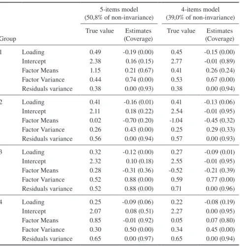
Table A.2 Monte Carlo Simulation for 5-item model and 4-item model. Check of 59 countries Alignment: True values, Estimates, and Coverage (in parentheses). Results for item v50 for the first four groups, N_g=1500.

5-items model

(50,8% of non-invariance) (39,0% of non-invariance)4-items model

Group True value (Coverage)Estimates True value (Coverage)Estimates

1 Loading 0.49 -0.19 (0.00) 0.45 -0.15 (0.00)

Intercept 2.38 0.16 (0.15) 2.77 -0.01 (0.89)

Factor Means 1.15 0.21 (0.67) 0.41 0.26 (0.24)

Factor Variance 0.44 0.74 (0.00) 0.53 0.67 (0.00)

Residuals variance 0.38 0.00 (0.93) 0.38 0.00 (0.94)

2 Loading 0.41 -0.16 (0.01) 0.41 -0.13 (0.06)

Intercept 2.11 0.18 (0.22) 2.54 -0.01 (0.95)

Factor Means 0.02 -0.70 (0.20) -1.04 -0.45 (0.32)

Factor Variance 0.26 0.43 (0.00) 0.25 0.29 (0.33)

3 Loading 0.32 -0.12 (0.00) 0.27 -0.09 (0.01)

Intercept 2.32 0.10 (0.18) 2.55 -0.01 (0.95)

Factor Means 0.28 -0.31 (0.36) -0.52 -0.21 (0.39)

Factor Variance 0.52 0.88 (0.00) 0.59 0.77 (0.00)

4 Loading 0.25 -0.09 (0.06) 0.22 -0.08 (0.19)

Intercept 2.07 0.08 (0.51) 2.27 0.00 (0.95)

Factor Means 0.85 -0.01 (0.92) 0.05 0.07 (0.80)

Factor Variance 0.30 0.50 (0.00) 0.34 0.45 (0.00)

(24)

Table A.3 Monte Carlo Simulation for 4-item model. Check of 47 and 34 coun-tries Alignment: True values, Estimates, and Coverage (in parenthe-sis). Results for item v50 for the first four groups, N_g=1500.

4-items model 47 countries

(26,9% of non-invariance) 4-items model 34 countries(21,0% of non-invariance)

Group True value (Coverage)Estimates True value (Coverage)Estimates

1 Loading 0.30 0.03 (0.96) 0.28 -0.03 (0.77)

Intercept 2.61 -0.20 (0.43) 2.47 -0.08 (0.73)

Factor Means -1.64 0.77 (0.22) -1.24 0.16 (0.90)

Factor Variance 0.47 -0.08 (0.76) 0.53 0.15 (0.96) Residuals variance 0.57 0.00 (0.93) 0.57 0.11 (0.96)

2 Loading 0.22 0.01 (0.98) 0.16 -0.03 (0.68)

Intercept 2.58 -0.12 (0.32) 2.86 -0.03 (0.72)

Factor Means -0.79 0.54 (0.23) -0.34 0.19 (0.61)

3 Loading 0.18 0.01 (0.91) 0.40 -0.06 (0.50)

Intercept 2.30 -0.10 (0.38) 2.44 -0.09 (0.59)

Factor Means -0.10 0.53 (0.27) -0.80 0.10 (0.84)

4 Loading 0.16 0.01 (0.95) 0.29 -0.05 (0.49)

Intercept 2.92 -0.08 (0.34) 1.86 -0.06 (0.56)

Factor Means -0.73 0.52 (0.25) -1.03 0.07 (0.64)

(25)

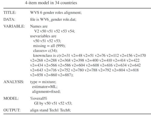
Table A.4 Mplus input excerpts for Fixed alignment ML estimation for the 4-item model in 34 countries

TITLE: WVS 6 gender roles alignment; DATA: file is WV6_gender role.dat; VARIABLE: Names are

V2 v50 v51 v52 v53 v54; usevariables are

v50 v51 v52 v53; missing = all (999); classes= c(34);

knownclass is c(v2=31 v2=48 v2=51 v2=76 v2=112 v2=156 v2=170 v2=268 v2=288 v2=368 v2=398 v2=400 v2=410 v2=414 v2=422 v2=434 v2=566 v2=586 v2=604 v2=608 v2=616 v2=634 v2=642 v2=643 v2=716 v2=752 v2=780 v2=788 v2=792 v2=804 v2=818 v2=858 v2=860 v2=887);

ANALYSIS: type = mixture; estimator=ML; alignment=fixed; MODEL: %overall%

(26)

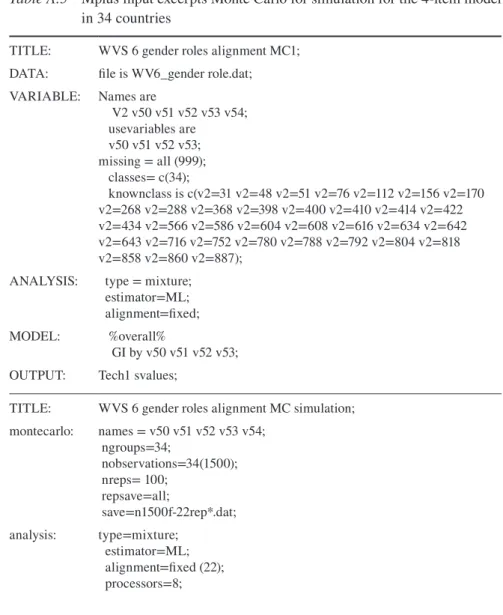
Table A.5 Mplus input excerpts Monte Carlo for simulation for the 4-item model in 34 countries

TITLE: WVS 6 gender roles alignment MC1; DATA: file is WV6_gender role.dat; VARIABLE: Names are

V2 v50 v51 v52 v53 v54; usevariables are

v50 v51 v52 v53; missing = all (999); classes= c(34);

knownclass is c(v2=31 v2=48 v2=51 v2=76 v2=112 v2=156 v2=170 v2=268 v2=288 v2=368 v2=398 v2=400 v2=410 v2=414 v2=422 v2=434 v2=566 v2=586 v2=604 v2=608 v2=616 v2=634 v2=642 v2=643 v2=716 v2=752 v2=780 v2=788 v2=792 v2=804 v2=818 v2=858 v2=860 v2=887);

ANALYSIS: type = mixture; estimator=ML; alignment=fixed; MODEL: %overall%

GI by v50 v51 v52 v53; OUTPUT: Tech1 svalues;

TITLE: WVS 6 gender roles alignment MC simulation; montecarlo: names = v50 v51 v52 v53 v54;

ngroups=34;

nobservations=34(1500); nreps= 100;

repsave=all;

save=n1500f-22rep*.dat; analysis: type=mixture;

(27)

model

population: %overall% gi by v50 -v53*1; %G#1%

gi BY v50*0.44755; gi BY v51*0.66271; gi BY v52*0.41177; gi BY v53*0.68205; [ v50*2.39376 ]; [ v51*2.10195 ]; [ v52*2.75848 ]; [ v53*2.01374 ]; [ gi*0 ]; v50*0.57993; v51*0.36809; v52*0.71822; v53*0.32406; gi*1; %G#2% […] Model: %overall%

gi by v50 -v53*1; %G#1%

gi BY v50*0.44755; gi BY v51*0.66271; gi BY v52*0.41177; gi BY v53*0.68205; [ v50*2.39376 ]; [ v51*2.10195 ]; [ v52*2.75848 ]; [ v53*2.01374 ]; [ gi*0 ]; v50*0.57993; v51*0.36809; v52*0.71822; v53*0.32406; gi*1;

(28)