Non-Randomized Response Models: An Experimental Application of the Triangular Model as an Indirect Questioning Method for Sensitive Topics

(1)

Non-Randomized Response Models:

An Experimental Application of the

Triangular Model as an Indirect

Questioning Method for Sensitive Topics

Anke Erdmann

Bielefeld University

Abstract

When it comes to sensitive questions, data is often affected by bias due to non-response or effects of social desirability. Several methods have been introduced to eliminate answer bias by using randomization processes and probabilistic theory to obscure the respondent’s answer and create anonymity, thus facilitating honest answers. The probably most tradi-tional method is the Randomized Response Technique by Warner (1965). However, this method is loaded with certain disadvantages. Therefore, in the last decade, newer meth-ods were introduced that aim at balancing the disadvantages and weaknesses of previous methods, for instance, the non-randomized models Crosswise Model and Triangular Model (Yu et al. 2008) as well as the Parallel Model (Tian 2014). Although especially the Trian-gular Model is easy to implement in a study, there is only little empirical evidence on its application in different survey modes and populations. Further, it is to assume that certain questions are not equally sensitive for everybody due to specific personal characteristics. Thus, indirect questioning might not be effective in general but only for certain popula-tions. The present study extends prior work on the Triangular Model by evaluating it for different subgroups. The conducted experiment asks for sensitive characteristics in the con-text of mental stress among students. The Triangular Model achieves significantly higher percentages than conventional direct questioning for illegal drug use among persons that answer socially desirable according to the characteristic of Self-Deception. For the other analyzed subgroups (Impression Management, gender, and depressiveness), the Triangular Model could not achieve higher prevalence rates compared to direct questioning on a suf-ficient probability level. But still, hard evidence on the effectiveness of indirect questioning models is thin and further critical discussion is needed.

Keywords: Triangular Model, Social Desirability, Indirect Questioning, Survey Method-ology, Non-Randomized Response

(2)

Acknowledgments

This research article is based on the author’s master thesis at the Faculty of Sociol-ogy at Bielefeld University. The author would like to thank Andreas Pöge (Faculty of Sociology, Bielefeld University) for the main supervision, Fridtjof Nußbeck (Faculty of Psychology and Sport Science, Bielefeld University) for the secondary supervision as well as the editors and the anonymous reviewers for their helpful and constructive com-ments on previous versions of this paper.

Direct correspondence to

Anke Erdmann, M.A., Faculty of Sociology, Bielefeld University, Universitätsstraße 25, 33615 Bielefeld

E-mail: [email protected]

Collecting data is substantial for empirical research. Yet, the reliability and validity of data gathered in surveys is at risk of being limited due to non-response, effects of social desirability or other bias. For that reason, continuous research in survey methodology is essential to further improve modes of data collection and anal-ysis. Especially social desirability has concerned scholars for some time now. It means that a respondent – deliberately or not – adjusts his or her answer according to what he or she thinks is socially accepted. Several scales have been developed to measure this construct and new interrogation techniques have been constantly introduced to take into account systematic bias in surveys. A promising possibility to collect data on sensitive topics is indirect questioning. Such techniques anony-mize the respondent’s answer using probability theory and try to facilitate honest answers by protecting the respondent’s information. Probably the most up-to-date techniques are so-called non-randomized response models. However, to this day, only few studies examine the performance and the viability of these methods. For some of those models, to the best of my knowledge, there is even no empirical testing at all. For this reason, this research article presents an evaluation of one selected non-randomized response model – the Triangular Model – that compares its estimated prevalence rates with the ones obtained with direct questioning.

The present study is mainly inspired by previous work by Jerke & Krumpal (2013) and aims at extending it by evaluating the Triangular Model in different subgroups. To test this assumption, an online survey was conducted in which the method was applied in the context of mental stress and psychological problems.

(3)

The Concept of Social Desirability

When conducting an empirical investigation, it is advisable to pay attention to effects of social desirability. A traditional scale to measure this answering behav-ior is the M-C SDS (Marlowe-Crowne Social Desirability Scale) by Crowne & Marlowe (1960). Redesigns for German studies are, for example, the SDS-CM (Social Desirability Scale by Crowne & Marlowe; Lück & Timaeus 1969, 1997b), the SDS-E (Social Desirability Scale by Edwards, Lück & Timaeus 1997a) and the SES-17 (Soziale Erwünschtheitsskala-17; Stöber 1999, 2001). These scales are easy to handle by using a summed score but there is criticism that they assume a one-dimensionality of the construct. In 1984, Paulhus argued that social desirabil-ity consists of two dimensions: Impression Management (IM) and Self-Deception (SD). Whereas IM means a deliberate deception to create a positive image towards others to gain social acknowledgment, SD describes the unconscious deception of one’s own to maintain an optimistic and positive self-image (Krumpal & Näher 2012; Paulhus 1984; Winkler et al. 2006). To measure those two dimensions, Paul-hus (1984) developed the Balanced Inventory of Desirable Responding (BIDR). Yet, this scale contains 40 items, which makes it inappropriate for most surveys. To overcome this, Winkler et al. (2006) developed a short scale that measures both dimensions of social desirability while containing only six items. The scale fulfills the criteria for reliability, internal and external validity and complies with the theo-retical and empirical assumptions of the BIDR-scale by Paulhus (1984). The scale’s formulation is described in the measurement section.

How strongly a question is affected by social desirability bias depends on the question’s content. A strong vulnerability to social desirability is given when a question is about sensitive, illegal or embarrassing content that is a potential danger for the respondent to reveal his or her true answer (e.g., sexuality, drug consump-tion, political opinions, violation of social norms). However, there is no exact defi-nition of what a sensitive question is. Tourangeau & Yan (2007) define it as follows:

“A question is sensitive when it asks for a socially undesirable answer, when it asks, in effect, that the respondent admits he or she has violated a social norm” (Tourangeau & Yan 2007, p. 860).

So in fact, the sensitivity of a question is not objective but depends on many factors (Wolter 2012). For instance, whether a question is sensitive or not might depend on who is asked. For example, Tourangeau & Yan (2007) mention political elections where the question whether someone voted or not is only sensitive for the ones who did not. Further, questions about political topics are more sensitive among higher educated people (Tourangeau & Yan 2007).

(4)

infor-mation about drug or alcohol consumption, in general, “no” seems to be the desir-able answer, but it is possible that within certain groups (e.g., among peers), “yes” is the more accepted answer. Additionally, whether a question is sensitive or not might depend on “who is asking.” For instance, being asked by a friend about sexu-ality or drug consumption is probably not as sensitive as being asked by a teacher, the parents or a research interviewer. Furthermore, it is possible that a question is differently biased in different subgroups. For example, questions about sexuality (e.g., number of sexual partners) might be equally sensitive for men and women but in opposite ways: While for one group, a high number is socially desirable, it is a low number for the other group. This extension that a question’s sensitivity depends on many circumstances is part of a definition by Porst (2009):

“A question is sensitive when the person answering it expects any negative responses of any kind as consequence of his or her answer in general or as consequence of a specific answer – this is independent from the content of the question” (Porst 2009, p. 124, own translation).

Therefore, a question is not sensitive per se but becomes sensitive through the situ-ation, the involved persons, and their expectations.

Indirect Questioning Models

(5)

are known. Hence it is obscured whether the sensitive characteristic applies. In this way, the general willingness to answer at all as well as the motivation to answer truthfully is expected to rise (Droitcour Miller 1981).

The RRT is well-researched and the body of literature offers many applica-tions and methodological evaluaapplica-tions on different sensitive topics (e.g., Coutts & Jann 2011; Kirchner et al. 2013; Abernathy et al. 1970; Pitsch et al. 2012). But, although many studies justify using the RRT by attesting its success (e.g., Lara et al. 2016; van der Heijden et al. 2016), there are also several investigations that provide evidence that the RRT fails to yield more valid estimates as compared to DQ (e.g., Beldt et al. 2016; Buchman & Tracy 1982; Wolter & Preisendörfer 2013). Some empirical studies further discuss a general failure of the technique due to incorrect following of the instructions and cheating. For example, Holbrook & Krosnick find that the RRT failed in reducing response bias because “respondents were either unable or unwilling to implement the randomized response technique properly” (2010, p. 328). This raises concerns about the viability of the RRT – especially in interview situations like online or telephone surveys that lack control whether the interviewees really use the randomization device. To investigate the effects of determinants of misreporting by question mode, Wolter & Preisendörfer (2013) conducted an experimental study with criminal convicts to compare direct questioning (henceforth: DQ) with RRT. Their findings include that “the success of the RRT varies systematically depending on the interview situation and the actors involved” (Wolter & Preisendörfer 2013, p. 344), which challenges the assumption of a general usefulness of the RRT. Further, the factors that determine response behavior vary by question mode. This finding might explain the mixed results on the performance of the RRT: If response behavior varies by certain characteris-tics, different compositions of analyzed samples lead to diverging results in spite of using the same technique. Additionally, besides mixed evidence, a key disad-vantage of RR-models is their complexity. The respondents have to understand the instructions and trust the procedure (Jann et al. 2012). Thus, cognitive overload, misunderstanding, and suspiciousness might result in answering errors (Jerke & Krumpal 2013). This and other weaknesses of RR-models shall be overcome by so-called non-randomized response models (NRR-models). The three techniques Crosswise Model, Triangular Model and Parallel Model are introduced in the fol-lowing section.

Crosswise Model

(6)

unequal.” The decisive element is that the probability distribution of the non-sensi-tive item is known (e.g., birth dates or random numbers like the last digit of a phone number). The model’s theoretical construction is shown in Figure 1. The parameter

a contains the unknown prevalence rate of the sensitive item and p is the probabil-ity to answer “yes” on the non-sensitive question.

The term s equal

(

" "

)

describes the share of “both answers are equal”-answers and is gathered from the sample. Thus, the estimator for the prevalence rate a – which is called aˆ_C for the CM in this paper – is the following (Jann et al. 2012; Yu et al. 2008):

(

" "

)

-1

, 0.5 2 -1

ˆ_C s equal p

a p

p

+

= ≠

⋅ (1)

ˆ_C

a = Estimated proportion of “yes”-answers on the sensitive item s = Proportion of “both equal”-answers in the sample

p = Probability of the non-sensitive item

The variance of the estimator can be obtained through the following formula (Jerke & Krumpal 2013; Tang et al. 2013; Yu et al. 2008; Liu & Tian 2014):

( )

₍

( )

₎

2

1-

, 0.5 2 -1

ˆ_C a a p p

Var a p

n _n _p

⋅ ⋅

= + ≠

⋅ (2)

The CM is a non-randomized version of Warner’s RRT (Tian 2014). It is character-ized by the same estimator, the same variance and is affected by the same math-ematical restrictions. The CM does also have the same qualities regarding the best possible choice for p and the same calculations of optimal sample size (Ulrich et al. 2012). The first empirical evaluation is by Jann et al. (2012), who use the method

(7)

for analyzing plagiarism and they compare the CM to DQ. Other methodological applications can be found in, for example, Kundt, Misch, & Nerré (2013) and Hoff-mann & Musch (2016).

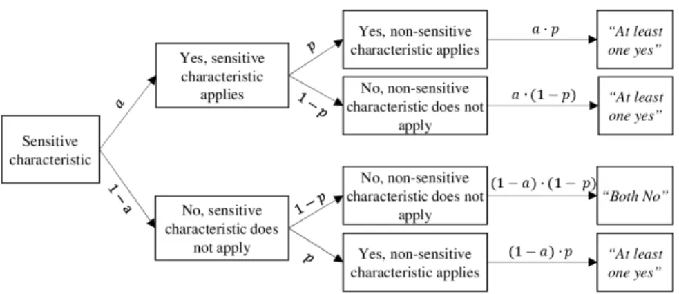
Triangular Model

The Triangular Model (TM) is similar to the CM but the essential distinction lies in the answering options. The sensitive question is once again linked to a non-sen-sitive characteristic with a known probability. But instead of choosing if either both answers are equal or not, the interviewee provides information whether his or her answers are both “no” or he or she affirms at least one of the two questions. Consid-ering these answConsid-ering options, a disadvantage in comparison with the CM becomes evident: The TM has an “option for protection.” Choosing “no on both questions” will definitely reveal that the respondent does not have the sensitive characteristic (Jann et al. 2012). So it can be criticized that the TM does not have a sufficient concealment of the answer “no” thus still being vulnerable to underreporting and the TM might not deliver adequate anonymization under certain circumstances (Tian 2014). Despite this drawback, the TM is worth testing because it surpasses other models regarding efficiency, revealment of the “yes”-answer, and is simple to implement in a survey (Wu & Tang 2016). Additionally, empirical evidence is rather scarce and it is still to be tested how this limitation really affects the model’s effectiveness.

An outline of the model can be seen in Figure 2. The proportion of “both no”-answers in the sample is the product of p’s inverse probability and the inverse proportion of the amount of persons carrying the sensitive item:

(

" "

) ( ) ( )

1-

1-s bothno = a ⋅ p (3)

(8)

Rearranging the term (3) provides the estimator aˆ_T for the TM (Jerke & Krumpal, 2013; Tang et al., 2013; Yu et al., 2008):

(

)

ˆ 1- " " 1-T s bothno

a

p

= (4)

ˆ_T

a = Estimated proportion of “yes”-answers on the sensitive item s = Proportion of “both no”-answers in the sample

p = Probability of the non-sensitive item

The estimator’s variance is described by the following formula (Jerke & Krumpal 2013; Tang et al. 2013; Yu et al. 2008):

( )

ˆ

( )

1-

_{( )}

( )

₁ 1

-T a a p a

Var a

n n p

⋅ ⋅

= +

⋅ (5)

These formulae reveal that the CM’s restriction of choosing a p other than 0.5 is eliminated for the TM. However, although Yu et al. (2008) do not exclude any prob-abilities mathematically1_{, a probability of 1 is not reasonable from a contentual} perspective. If the probability of the non-sensitive item is 1 (i.e., the respondent’s answer is definitely “yes”), the answer “both no” is not possible. Thus, all respon-dents have to answer with “at least one yes” so an estimation of the prevalence rate is impossible since the proportion of “both no”-answers is always 0 independently from the true prevalence rate a. In this case, total anonymity is given but also no result.

The opposite case of p=0 is not advisable as well: If the answer on the non-sensitive item is definitely “no,” then it is clear that “at least one yes” means a “yes” on the sensitive question. Regarding the estimator and its variance, this means that the parts containing p are cancelled. So in fact, a TM with p=0 is basically just direct questioning resulting in total revelation of the answers but no anonymity. In conclusion, it is advisable to choose a probability that balances the relation between anonymity and efficient estimation.

To my best knowledge, the only application of the model is by Jerke & Krump-al. (2013) on student plagiarism at a German university. The study reveals higher prevalence rates for partial as well as for full plagiarism. In comparison to the CM, the authors find a smaller standard error for the TM and thus a more efficient esti-mation. However, the differences achieved with the TM are not significantly higher than in DQ.

(9)

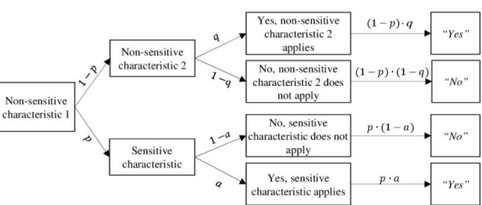
Parallel Model

Despite the advantages of the CM and the TM, they both have a certain limita-tion: one category (usually the “no”-answer) has to be non-sensitive (Tian 2014, p. 293). To eliminate this restriction, Tian (2014) introduces another NRR-model: the Parallel Model (PM). This technique uses two non-sensitive items with a known probability (named as W and U). The respondents belong to two groups (W=1 and W=0, i.e., the first non-sensitive characteristic applies or not). Then, the answer on this first non-sensitive question (W) decides whether the respondent answers the second non-sensitive (U) or the sensitive question (Y) (for an example, see Tian 2014, p. 300). Since the answer on the first question is unknown, the interviewer does not know which question is answered. Figure 3 shows an outline of the PM and how the amount of “yes” and “no” answers in the sample is composed. From this Figure, the following estimator can be derived (Tian 2014, p. 301):

(

" " -

) ( )

1-ˆ_P s yes q p

a

p

⋅

= (6)

ˆ_P

a = Estimated proportion of “yes”-answers on the sensitive item s = Proportion of “yes”-answers in the sample

p, q = Probabilities of the non-sensitive items

Again, the estimator’s variance consists of the usual sampling variance and addi-tionally a part that is induced by the randomization process.

( )

( ) (

)

2

1 1

ˆ_P a a p

Var a

n n p

ϕ

⋅ − − ⋅

= +

⋅

where _{ϕ =}

( )

_p_-1_{⋅ +}_q2

(

_{1- 2}_{⋅ ⋅ ⋅ + ⋅}_{a p q a p}

)

₍₇₎

(10)

The combination of answers leads to a parallelism (for more details, see Tian 2014, p. 300) which is displayed in Figure 4 alongside the answering options for the CM and TM.

The logic of the PM is comparable to the Unrelated Question Model by Hor-vitz et al. (1967). Thus, the PM combines the advantages of this specific RR-model with the strengths of an NRR-model: The design is a device-free technique but has – compared to the CM and the TM – a better anonymization of answers. The infor-mation whether the sensitive characteristic applies or not are both protected. So far, to the best of my knowledge, there are no experimental applications that evaluate the PM in comparison to DQ.

The Present Study

Inspired by the work of Jerke & Krumpal (2013), the present study examines the TM by comparing its estimated prevalence rates to the ones that are achieved using DQ. It is assumed that anonymized questioning “cancels out the costs that make respondents misreport in DQ mode” (Wolter & Preisendörfer 2013, p. 329). This includes persons that strive for social acknowledgment, thus answering socially desirable. Further, several authors point out that misreporting in surveys is most likely for the persons who “have the most to lose” when reporting truthfully (Ber-nstein et al. 2001; Wu & Tang 2016), i.e., the persons that have the sensitive char-acteristic. Thus, this study puts the focus on the assumption that a question might have different levels of sensitivity for different persons or groups, so the TM might prove to be efficient only in certain subgroups in the sample. For this purpose, an online survey on the topic “Mental stress among students” was conducted (field time from 13th_{to 27}th_{July 2015). First, the TM is compared to DQ in general.}

(11)

Since the answers are anonymized when using the TM, a higher prevalence rate can be expected in comparison to DQ because a more honest answering behavior is assumed (Hypothesis 1).

Second, the TM will be analyzed separately for gender (Hypothesis 2), social desirability (with the two dimensions IM and SD; Hypothesis 3), and depressive-ness (Hypothesis 4). Regarding social desirability, a stronger effect of the indirect questioning method is assumed for persons who have the characteristic of answer-ing socially desirable. But, it is expected that the anonymization is only effective for IM. Deceiving according to IM is a conscious act to create a more positive image of oneself, for instance, in an interview situation. Self-deceptive behavior, however, is subconscious. Thus, anonymization of an interview situation should not affect the bias created by this characteristic. Regarding depressiveness, in the present study, the TM is supposed to be more efficient for persons with a high level of depressive-ness because the questions in this specific questionnaire are assumed to be more sensitive for this group than for persons who are not depressive. The effect that is postulated for gender is assumed to be indirect. Prior research indicates that social desirability varies by gender. Females are more prone to answer socially desir-able (Becker & Cherny 1994; Dalton & Ortegren 2011) – especially regarding IM. Further, studies suggest that female students are more strongly strained by depres-siveness than their male colleagues (Burger & Scholz 2018; Margitics & Pauwlik 2009). Thus, it is assumed that the TM works better for females.

The questionnaire was conducted as an online survey because this method offers advantages considering the possibility to contact many people and to ran-domly sort the respondents into the two survey conditions.

Measurements

Sensitive Questions

According to the topic of mental stress amongst students, the respondents were asked whether they ever did the following acts during their studies:

Did you ever make use of a psychological consultancy?

Did you ever use prescriptive medication for enhancing mental performance?2

Did you ever use illegal drugs for enhancing mental performance?3

2 Additional explanation: “For example, to learn more fastly and efficiently, to manage a workload or to be more focused during an exam.”

(12)

Respondents in the DQ condition received the questions as they are and were asked to answer with “yes” or “no.” For the TM, the questions were combined with the following non-sensitive questions:

Is your mother’s birthday in January, February, or March? Is your birthday in May?

Is your birthday in January?

The two possible answering options were:

The answer is “no” on both questions.

The answer is “yes” on at least one of the questions.

Independent Variables

The concept of social desirability was measured using the scale by Winkler et al. (2006). The scale contains six items that represent both dimensions of social desir-ability, Impression Management (IM) and Self-Deception (SD). Table 1 shows the wording of the items and which dimension is measured. The notes + and – depict whether a high or a low value represents the tendency to answer socially desirable.

To check for the scale’s dimensionality, a principal component factor analysis

(PCA; Bortz 1989) was performed. The PCA confirms two factors and also the polarity assumed by Winkler et al. (2006). The results are in line with the findings by the authors and reflect the scale’s theoretical assumptions.

In consideration of the items’ polarity, two mean indices are designed for IM and SD by summing up the values of the items and dividing by their number. The correlation between the two dimensions is rather low (r=0.13, p=0.000), which confirms that these are two distinct concepts which are only slightly correlated. According to Paulhus, only extreme answers can be interpreted as socially desir-able answering behavior. Thus, for each dimension, two subgroups are constructed using the same method as Winkler et al. (2006) by generating a dichotomous vari-able where values of 6 and higher are marked as 1 and all other values below this line are marked as 0.

Depressiveness is operationalized using a scale from Mohr & Müller (2014) which contains eight items that measure depressiveness in a non-clinical context (Table 2).

(13)

not define a cut point that marks depressiveness, the values 5, 6, and 7 (often, very often, and almost always) are coded to indicate a high level of depressiveness.

The collected demographic information are age and gender. For gender, the respondents could choose between male, female, and other. The information on age is used to refine the probability of the non-sensitive questions in the TM (see below). The questions were placed at the end of the questionnaire. No further demographic information were retrieved to keep the survey short and parsimonious.

Table 2 Depressiveness scale by Mohr & Müller (2014)

Instruction: Use the following answering options to state whether resp. how often the fol-lowing statements apply to you. There is no right or wrong answer. Please do not leave out any questions!

I have to push myself to do things. Many things seem pointless to me. I am oppressed by feelings of guilt.

I feel lonely even when I am around other people. I have sad moods.

It is hard for me to make decisions. At the beginning of the day, I feel worst. I look into the future without hope.

Note: Own translation, answering options: 1=never, 2=very rarely, 3=rarely, 4=occasionally, 5=often, 6=very often, 7=almost always.

Table 1 Operationalized BIDR short scale by Winkler et al. (2006)

Instruction: Please take position to the following behaviors. What would you say: To what extent does the sentence apply to you?

My first impression of people usually turns out to be right. SD +

I am often insecure in my judgment. SD –

I always know why I like things. SD +

I have received too much change from a salesperson without telling him or her. IM –

I am always honest to other people. IM +

There have been occasions when I have taken advantage of someone. IM –

(14)

Sampling and Data Collection

As apparent from the previous description, the variance for the estimators of indi-rect questioning models is always inflated due to an additional variance induced by the randomization process. So there is a need for a preferably large sample size to oppose the inaccuracies accompanied by the increased standard errors. Therefore, a main objective was to reach a large number of participants. The call to participate in the survey was sent to students via diverse mail distribution systems at different universities in Germany. First, ten public universities were chosen non-randomly. Then, e-mails were sent out to persons in charge (e.g., secretaries at the dean offices) at all faculties, resp. institutes at these selected universities. Thus, there is no spe-cialization and all kinds of study programs are included. This way, a total sample size of n=1,546 was achieved for this study.4

Table 3 shows the sample size by the two survey conditions DQ and TM as well as for gender.5_{It is obvious that there is a bias regarding the distribution by males} and females: Around 70% of respondents are female. The reason for this discrep-ancy is unclear. It is unlikely that this relation reflects the true gender distribution in the general population or distribution at the universities since a broad variety of study programs was selected. Instead, it is possible that this is the result of a higher willingness for females to participate in studies as well as a greater interest in sur-veys about psychological problems. This bias is considered to be irrelevant for the present experimental study, thus the data will be analyzed as it is.

4 All in all, 230 persons aborted the online survey before reaching the experimental part of the questionnaire where the random sorting into DQ and TM condition takes place. Thus, the following analyses are based on a sample of 1,316 persons.

5 The group of persons that report other as their gender will not be considered as a sepa-rate group in the following gendered analysis due to very low sample size.

Table 3 Sample size by survey condition and gender

Total Gender

Female Male Other N.A.

Direct Questioning 688 478 196 13 1

Triangular Model 628 448 163 15 2

Total 1,316 926 359 28 3

(15)

Analytical Strategy

The TM will be evaluated by estimating the prevalence rates using the formu-lae presented above. Additionally, the differences between the prevalence rates achieved with TM and DQ will be examined. These differences will be tested for statistical significance using the following formula (Jerke & Krumpal 2013, p. 364):

( )

(

)

- 1-ˆ ˆ

ˆ ˆ ˆ

T D

D D

T

D

a a t

a a

Var a

n

=

⋅ +

(8)

The parameters aˆ_T and Var a

( )

ˆ_T have been described before. The abbreviation aˆ_D marks the prevalence rate estimated with direct questioning (with nD as belong-ing sample size). The distribution is the Student t-Distribution with nD+ 2nT − degrees of freedom.

The probabilities of the non-sensitive questions in the TM were determined based on data from the German Federal Statistical Office using age, resp. the birth year of the respondents. For this, the individual probability for each person was estimated by considering the birth rates of males and females for each month within a certain year. Then, the average was calculated for the whole sample. The probability for the mother’s birth month was determined in the same way. Prior to this, however, the mother’s birth year was estimated based on the respondent’s birth year and the average age a mother gave birth to a child. Thus, the probabilities for the non-sensitive characteristics in this specific sample are the following:

“Is your mother’s birthday in January, February, or March?” p=0.258

“Is your birthday in May?” p=0.084

“Is your birthday in January?” p=0.085

Additionally, to analyze whether the TM works differently in certain groups of respondents, the differences-in-differences (DID) are considered. Analyzing DID is a technique to identify causal relationships by examining the influence of a cer-tain treatment (Bertrand et al. 2003). Usually, it analyzes two groups – one group receives a treatment and the other group does not – that are measured at two time points. Then, the difference between the two time points of measurement within

(16)

(

TM DQ-

)

_Subgroup₁-

(

TM DQ-

)

_Subgroup₂ (9)

If this difference-in-differences turns out to be non-random, this would suggest that the difference can be traced back to the subgroup, i.e., the TM works differently in the compared subgroups.

Results

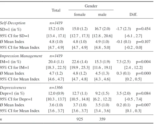
Table 4 shows the descriptive results of the three main independent variables by gender. According to this dichotomization, 15.2 percent of the persons in the sam-ple feature the characteristic of SD. Regarding IM, the proportion of persons classi-fied as having this characteristic amounts to 20.4 percent.

Table 4 Proportions and means for Self-Deception, Impression Management and depressiveness by gender

Total Gender

female male Diff.

Self-Deception n=1419

SD=1 (in %) 15.2 (1.0) 15.0 (1.2) 16.7 (2.0) -1.7 (2.3) p=0.454 95% CI for SD=1 [13.4 , 17.1] [12.7 , 17.3] [12.8 , 20.6] [-6.1 , 2.7] Ø Mean Index 4.8 (1.0) 4.8 (1.0) 4.9 (1.0) -0.1 (0.1) p=0.107 95% CI for Mean Index [4.7 , 4.9] [4.7 , 4.9] [4.8 , 5.0] [-0.2 , 0.0]

Impression Management n=1419

IM=1 (in %) 20.4 (1.1) 22.6 (1.4) 15.3 (1.9) 7.3 (2.5) p=0.004 95% CI for IM=1 [18.3 , 22.5] [19.9 , 25.3] [11.6 , 19.1] [2.4 , 12.2] Ø Mean Index 4.7 (1.2) 4.8 (1.2) 4.5 (1.3) 0.3 (0.1) p=0.000 95% CI for Mean Index [4.6 , 4.7] [4.7 , 4.8] [4.3 , 4.6] [0.2 , 0.5]

Depressiveness n=1366

Depr=1 (in %) 12.0 (0.9) 12.7 (1.1) 9.2 (1.5) 3.5 (2.0) p=0.084 95% CI for Depr=1 [10.3 , 13.7] [10.5 , 14.8] [6.2 , 12.2] [-0.5 , 7.4] Ø Mean Index 3.6 (1.0) 3.7 (1.0) 3.5 (1.0) 0.2 (0.1) p=0.007 95% CI for Mean Index [3.6 , 3.7] [3.6 , 3.7] [3.4 , 3.6] [0.1 , 0.3]

n 925 359

(17)

Men feature a slightly higher proportion of SD than women, but this difference is not statistically significant on a 5%-level. For IM, however, there is a considerably and significantly (p=0.004) higher share for female persons. Similar results about gender differences for these two dimensions were found by other authors as well (Becker & Cherny 1994; Winkler et al. 2006).

Regarding the average depressiveness by gender, it becomes evident that female students feature a rather slightly but significantly higher level of depressive-ness compared to male students. The dichotomized variable shows that the propor-tion of persons classified as depressive is more than three percentage points higher, but not significantly, among females.

Indirect Questioning – Full Sample Analysis

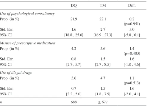
Table 5 shows the prevalence rate for the sensitive questions when asking directly as well as the rates that were estimated using the TM. The results show that the indirect questioning model reveals slightly higher percentages for the sensitive

Table 5 Prevalence rates of the sensitive questions

DQ TM Diff.

Use of psychological consultancy

Prop. (in %) 21.9 22.1 0.2

(p=0.951)

Std. Err. 1.6 2.7 3.0

95% CI [18.8 , 25.0] [16.9 , 27.3] [-5.8 , 6.1]

Misuse of prescriptive medication

Prop. (in %) 4.2 5.6 1.4

(p=0.403)

Std. Err. 0.8 1.5 1.6

95% CI [2.7 , 5.7] [2.7 , 8.5] [-1.8 , 4.6]

Use of illegal drugs

Prop. (in %) 3.6 4.7 1.1

(p=0.513)

Std. Err. 0.7 1.5 1.6

95% CI [2.2 , 5.0] [1.8 , 7.5] [-2.0 , 4.1]

n 688 ≥ 627

(18)

questions. However, none of these differences turn out to be statistically significant. Hence, the TM does not achieve higher estimates when analyzing the total sample of students.

Indirect Questioning – Subgroup Analysis

According to the assumption that a question might only be sensitive for a certain group of people, the TM’s effectiveness is checked within subgroups. As stated in the hypotheses section, the analysis is conducted for gender, the two dimensions of social desirability, and depressiveness.

Gender

The results with respect to gender are displayed in Table 6. The TM reveals slightly higher estimates for females but the differences between the survey conditions are small and not statistically significant. Although the differences between TM and DQ are larger for males, the effect is not significant as well. Thus, for these two subgroups, the indirect questioning model could not achieve non-randomly higher

Table 6 Prevalence rates of the sensitive questions by gender

Female Male

DQ TM Diff. DQ TM Diff.

Prop. (in %) 23.4 25.7 2.3

(p=0.535) 16.8 10.8 (p=0.283)-6.1

Std. Err. 1.9 3.2 3.7 2.7 5.0 5.4

95% CI [19.6 , 27.2] [19.5 , 31.9] [-4.9 , 9.5] [11.6 , 22.1] [0.9 , 20.6] [-16.8 , 4.6]

Prop. (in %) 4.8 5.0 0.2

(p=0.932) 2.6 6.3 (p=0.248)3.7

Std. Err. 1.0 1.7 2.0 1.1 3.0 3.0

95% CI [2.9 , 6.7] [1.6 , 8.4] [-3.7 , 4.0] [0.3 , 4.8] [0.4 , 12.1] [-2.2 , 9.6]

Prop. (in %) 2.5 2.7 0.2

(p=0.913) 5.6 10.9 (p=0.159)5.3

Std. Err. 0.7 1.6 1.7 1.6 3.3 3.5

95% CI [1.1 , 3.9] [-0.5 , 5.9] [-3.2 , 3.6] [2.4 , 8.9] [4.3 , 17.4] [-1.7 , 12.2]

n 478 448 196 163

(19)

percentages for the sensitive questions. As opposed to the theoretical assumptions, the TM even yielded a lower prevalence rate than DQ among men for the question of psychological consultancy.

Since the TM achieves a higher prevalence rate than DQ for females while yielding a lower rate for males, the DID between females and males amounts to 8.4 percentage points for the first question. As to be seen in Table 7, the discrepan-cies of the survey conditions’ differences between the subgroups are lower for the other two questions and also reversed (the TM achieves higher prevalence rates for men). However, none of these DID reach a sufficient level of statistical significance. Therefore, a systematic influence of gender on the TM’s performance cannot be supported.

Social Desirability

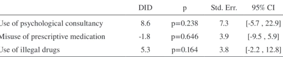
Further, the analysis is conducted for the two dimensions of social desirability of which the results are displayed in Table 8 and Table 10. For persons that answer socially desirable according to IM, it becomes evident that the TM achieves higher percentages of persons having the sensitive characteristics. For example, the preva-lence rate of using a psychological consultancy is seven percentage points higher when asking the question indirectly using the TM. However, this difference fails to achieve statistical significance. A similar difference can be found for the use of illegal drugs: When asking directly, only 0.8 percent of the persons admit to hav-ing used drugs durhav-ing their studies. When asked ushav-ing the TM, 6.1 percent in this subgroup state having used illegal drugs to enhance mental performance. However, none of these differences turn out to be statistically significant on a p≤0.05 level. Regarding the subsample of persons not having the characteristic of IM, no relevant or significant effect of the indirect questioning model can be found.

Although the TM yields higher estimates for the IM=1 group for the first and third question, the DID, as portrayed in Table 9, show no statistical significance. Thus, considering the DID is also in line with the finding that the TM’s estimates

Table 7 Differences-in-differences for gender

DID p Std. Err. 95% CI

Use of psychological consultancy 8.4 p=0.227 6.9 [-5.2 , 22.0] Misuse of prescriptive medication -3.5 p=0.355 3.8 [-10.9 , 3.9]

Use of illegal drugs -5.1 p=0.148 3.5 [-12.0 , 1.8]

(20)

Table 8 Prevalence rates of the sensitive questions by social desirability: Impression Management

IM=1 IM=0

Prop. (in %) 20.9 27.9 7.0

(p=0.298) 22.2 20.6 (p=0.643)-1.6

Std. Err. 3.6 5.7 6.8 1.8 3.0 3.4

95% CI [13.8 , 28.0] [16.8 , 39.0] [-6.5 , 20.5] [18.7 , 25.6] [14.7 , 26.5] [-8.2 , 5.0]

Prop. (in %) 2.3 2.4 0.1

(p=0.990) 4.7 6.6 (p=0.321)1.9

Std. Err. 1.3 2.8 3.2 0.9 1.7 1.9

95% CI [-0.3 , 5.0] [-3.1 , 7.9] [-6.3 , 6.4] [2.9 , 6.4] [3.2 , 10.0] [-1.8 , 5.6]

Prop. (in %) 0.8 6,1 5.3

(p=0.105) 4.3 4.3 (p= 0.999)0.0

Std. Err. 0.8 3.2 3.4 0.9 1.6 1.8

95% CI [-0,8 , 2.3] [-0.1 , 12.4] [-1.4 , 12.1] [2.6 , 6.0] [1.1 , 7.5] [-3.5 , 3.5]

n 129 142 559 ≥ 484

Note: In case of differences, the least number of observations is displayed; n for TM and IM=0: 485, 485, 484; DQ=Direct Questioning, TM=Triangular Model, Prop. (in %)=(Estimated) proportion of “yes”-answers, Std. Err.=Standard Error, 95% CI=95% Confidence Interval.

Table 9 Differences-in-differences for social desirability: Impression Management

Use of psychological consultancy 8.6 p=0.238 7.3 [-5.7 , 22.9] Misuse of prescriptive medication -1.8 p=0.646 3.9 [-9.5 , 5.9]

Use of illegal drugs 5.3 p=0.164 3.8 [-2.2 , 12.8]

(21)

do not systematically differ from DQ and there is also no effect that could be traced back to socially desirable answering behavior according to IM.

As stated earlier, it is assumed that effects of the TM could only be found for IM but not for SD, since SD is not a deliberate form of deception. The estimated percentages show that no significant effects can be found for persons that do not feature the characteristic of SD (Table 10) and the differences between the survey conditions are small. For persons in subgroup SD=1, the TM yields lower percent-ages as DQ for the first two questions but also not on a statistically significant level. However, there is a considerably and statistically significant higher prevalence rate for use of illegal drugs when using the TM (12.6 percent as compared to 3.0 percent using DQ). In fact, the SD=1 group even shows the highest percentage of drug consumption compared to all other subgroups when asking indirectly. These results are reasonable on the assumption of the personality that is ascribed to

per-Table 10 Prevalence rates of the sensitive questions by social desirability: Self-Deception

SD=1 SD=0

Prop. (in %) 16.8 12.4 -4.4

(p=0.557) 22.8 24.1 (p=0.712)1.3

Std. Err. 3.7 6.5 7.4 1.7 2.9 3.3

95% CI [9.4 , 24.3] [-0.2 , 25.1] [-19.0 , 10.3] [19.4 , 26.2] [18.4 , 29.8] [-5.2 , 7.7]

Prop. (in %) 5.0 1.8 -3,2

(p= 0.419) 4.1 6.4 (p=0.217)2.3

Std. Err. 2.2 3.3 3.9 0.8 1.7 1.8

95% CI [0.6 , 9.3] [-4.7 , 8.2] [-10.9 , 4.6] [2.5 , 5.7] [3.1 , 9.6] [-1.2 , 5.8]

Prop. (in %) 3.0 12.6 9.6

(p=0.042) 3.7 3.2 (p= 0.755)-0.5

Std. Err. 1.7 4.4 4.7 0.8 1.5 1.7

95% CI [-0.4 , 6.3] [4.0 , 21.2] [0.4 , 18.9] [2.2 , 5.3] [0.2 , 6.2] [-3.8 , 2.7]

n 101 100 587 ≥ 526

(22)

sons with a high level of SD: First of all, a certain level of SD characterizes a psychologically stable person and a positive self-image (Winkler et al. 2006, p. 3). This is also reflected in the amount of persons that used a psychological consul-tancy, which is rather low among persons with SD=1 (16.8 percent). Also, this is supported by a negative correlation between the mean indices for Self-Deception and depressiveness in this sample (r= –0.31, p=0.000). It is conceivable that per-sons with a high level of SD are also very outgoing and adventurous, thus having a higher tendency toward behavior like drug consumption. Therefore, this question might be especially sensitive to these persons because they are the ones that tend to misuse drugs. This could explain why there is a significant effect of the TM for this subgroup although it is not theoretically assumed according to social desirability.

Regarding the discrepancies between the differences in the survey conditions, it is evident for the first and second question that the TM mostly achieves only slightly higher estimates or even lower percentages which is also reflected in the DID (Table 11). As a consequence, for questions 1 and 2, there is no evidence for an influence of SD on the survey conditions’ estimates. However, for the question about use of illegal drugs, also the DID shows to be statistically significant on the conventional 5%-level. Therefore, it can be concluded that the TM achieves a higher prevalence rate for persons with a high level of self-deceptive attitudes and there is evidence that the model works differently for these two SD groups.

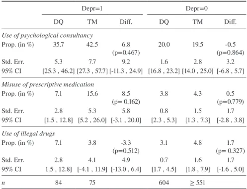
Depressiveness

As compared to the other subgroups, the prevalence rate of using a psychological consultancy is highest among students that are classified as depressive (35.7 per-cent). The TM increases this percentage by nearly seven percentage points. Fur-ther, the percentage for misuse of prescriptive medication is nearly nine percentage points higher when asking indirectly instead of directly (Table 12). But these differ-ences between the survey conditions are not statistically significant. For the use of illegal drugs, the TM cannot achieve a higher prevalence rate for this subgroup. In fact, the estimation is even slightly lower. Further, there are only marginal and no

Table 11 Differences-in-differences for social desirability: Self-Deception

Use of psychological consultancy -5.7 p=0.489 8.2 [-21.9 , 10.5] Misuse of prescriptive medication -5.5 p=0.219 4.5 [-14.3 , 3.3]

Use of illegal drugs 10.1 p=0.022 4.4 [1.5 , 18.7]

(23)

significant differences between direct and indirect questioning for the subsample of persons that are not depressive.

So although the TM generates higher prevalence rates for the first and second sensitive question, there is no effect of depressiveness on the model’s performance as suggested by the DID in Table 13. None of the discrepancies is significant on the conventional level. Therefore, it cannot be concluded that the indirect questioning technique might work differently for persons that are classified as depressed when asking sensitive questions about mental stress.

Table 12 Prevalence rates of the sensitive questions by depressiveness

Depr=1 Depr=0

Prop. (in %) 35.7 42.5 6.8

(p=0.467) 20.0 19.5 (p=0.864)-0.5

Std. Err. 5.3 7.7 9.2 1.6 2.8 3.2

95% CI [25.3 , 46.2] [27.3 , 57.7] [-11.3 , 24.9] [16.8 , 23.2] [14.0 , 25.0] [-6.8 , 5.7]

Prop. (in %) 7.1 15.6 8.5

(p= 0.162) 3.8 4.3 (p=0.779)0.5

Std. Err. 2.8 5.3 5.8 0.8 1.5 1.7

95% CI [1.5 , 12.8] [5.2 , 26.0] [-3.1 , 20.0] [2.3 , 5.3] [1.3 , 7.3] [-2.8 , 3.8]

Prop. (in %) 7.1 3.8 -3.3

(p=0.512) 3.1 4.8 (p= 0.327)1.7

Std. Err. 2.8 4.1 4.9 0.7 1.6 1.7

95% CI 1.5 , 12.8] [-4.1 , 11.9] [-13.0 , 6.4] [1.7 , 4.5] [1.8 , 7.9] [-1.6 , 5.0]

n 84 75 604 ≥ 551

(24)

Conclusion and Discussion

Regarding the full sample, the analysis revealed that there is no significant differ-ence in the percentages achieved by the TM as compared to DQ. The same results can be found for gender: Although differences were expected for females, no sig-nificant higher prevalence rate could be achieved by the TM. Thus, there is no evidence for hypotheses 1 and 2.

Regarding social desirability, the TM could achieve higher percentages in the IM=1 group, but not in a statistically significant way. Although not expected, there is a significant higher prevalence rate for drug use within the group with the char-acteristic of SD. Testing the DID reveals that this performance of the TM differs significantly in this subgroup. Therefore, hypothesis 3 can be partially supported: An effect can be found for one of thedimensions of social desirability but not for the one that was theoretically assumed. Further, the effect can only be found for one of the three questions.

Within the group that is classified as depressed, higher prevalence rates can be found for usage of psychological consultancy and misuse of prescriptive medica-tion, but again not on a sufficient probability level. Thus, no empirical valid support for hypothesis 4 can be found.

In conclusion, the evidence for the postulated assumptions and hypotheses is rather thin. Further, there are some limitations regarding the methodological per-spective. First, it has to be stated that the results are not representative and the numbers of observations in the subgroups are small. A sample of university stu-dents was used and the mode of data collection was an online survey. Hence, the sample’s representativeness is affected by selection through the mail distribution system, through online access, resp. internet affinity, and through self-selection (e.g., willingness to participate in a survey). Therefore, it should be kept in mind that the results are not transferrable to a general population but only to this very

Table 13 Differences-in-differences for depressiveness

Use of psychological consultancy 7.3 p=0.434 9.3 [-11.0 , 25.6] Misuse of prescriptive medication 8.0 p=0.116 5.1 [-2.0 , 18.0]

Use of illegal drugs -5.0 p=0.313 4.9 [-14.7 , 4.7]

(25)

specific sample. Hence, there is still the need to evaluate the technique in other, more general samples and with other modes of data collection.

Another criticism – not only in this study but also in general – is that we can-not know whether the participants follow the instructions of the TM. Although it is unknown as well in DQ mode whether the respondents lie or tell the truth, indi-rect questioning methods might be especially vulnerable to deliberate cheating due to distrust. Very recently, Wu & Tang (2016) discussed noncompliance in NRR-models. They argue that especially the persons that “have the most to lose” (Wu & Tang 2016, p. 2828), i.e., the persons that carry the sensitive characteristic, tend to answer falsely due to distrust in the technique. As mentioned earlier in this paper, the TM has a clear protective answer (“both no”) so it might be especially sensitive to cheating that would result in underreporting thus concealing the model’s effec-tiveness. For that reason, the authors introduce the dual non-randomized response triangular model (DNRRTM) and the alternating non-randomized response trian-gular model (ANRRTM). In the DNRRTM, the respondents are randomly assigned to two groups where each group gets a different non-sensitive question combined with the sensitive question of interest. Thus, two non-sensitive characteristics with known probabilities are needed. The ANRRTM, however, functions with only one non-sensitive question where the two categories are alternated in the two groups. In a test of their models, Wu & Tang (2016) find that the DNRRTM as well as the ANRRTM provide higher prevalence rates compared to the TM. The authors rec-ommend the ANRRTM since it is easier to implement by using only one innocuous question.

These results are useful regarding the results of the present study. Wu & Tang (2016) argue that the TM underestimates the true prevalence rate due to deliberate cheating especially by those who have the sensitive characteristic. In this study, the main assumption was that the TM is especially efficient for subgroups that are somehow related with the sensitive question or social desirability (e.g., depressed persons and questions about psychological consulting). In conclusion, it would be a possible perspective for future research to combine these two findings and to test the improved ANRRTM with regard to relevant subgroups.

(26)

hav-ing the sensitive characteristic). In their validation studies, they show that the CM produces “false positives to a nonignorable extent” (Höglinger & Diekmann 2017, p. 135) which challenges the assumption that higher estimates are more valid. Even further, it calls into question the CM’s good performance that has been suggested in previous studies. It is possible that these studies are biased by these false positives that inflate the model’s estimates. Overall et al. (2018, p. 1) summarize that, in their study, none of the three tested indirect questioning models subtantially outperform direct questioning.

In conclusion, the authors speak against relying blindly on the more-is-better-assumption (Höglinger & Diekmann 2017, p. 136) which has been most prominent when examining (non-) randomized response models. Instead, validation strate-gies should be considered to evaluate indirect questioning models more accurately. In this paper, the validity and performance of the TM was also mainly judged in comparison to direct questioning. Therefore, future studies that evaluate this NRR-model might surely benefit from using validation data as it is suggested in current studies. In summary, the present study cannot deliver evidence for the hypothesis that indirect questioning models might be more effective in certain subgroups but it provides hints that a more precise analysis might be fruitful. We should improve future research on that topic and encourage further theoretical and empirical dis-cussion on randomized and non-randomized response models.

References

Abernathy, J. R., Greenberg, B. G., & Horvitz, D. G. (1970). Estimates of Induced Abortion in Urban North Carolina. Demography, 7(1), 19–29.

Barton, A. H. (1958). Asking the Embarrassing Question. Public Opinion Quarterly, 22(1), 67–68.

Becker, G., & Cherny, S. S. (1994). Gender-controlled measures of socially desirable re-sponding. Journal of Clinical Psychology, 50(5), 746–752. https://doi.org/10.1002/1097-4679(199409)50:5<746::AID-JCLP2270500512>3.0.CO;2-V

Beldt, S. F., Daniel, W. W., & Garcha, B. S. (2016). The Takahasi-Sakasegawa Randomized Response Technique. Sociological Methods & Research, 11(1), 101–111. https://doi.org /10.1177/0049124182011001006

Bernstein, R., Chadha, A., & Montjoy, R. (2001). Overreporting Voting: Why It Happens And Why It Matters. Public Opinion Quarterly, 65, 22–44.

Bertrand, M., Duflo, E., & Mullainathan, S. (2003). How Much Should We Trust Differenc-es-In-Differences Estimates? NBER Working Paper Series, 8841. Cambridge, Massa-chusetts: National Bureau of Economic Research.

Bortz, J. (1989). Statistik für Sozialwissenschaftler. Heidelberg: Springer.

(27)

Burger, P. H. M., & Scholz, M. (2018). Gender as an underestimated factor in mental health of medical students. Annals of Anatomy = Anatomischer Anzeiger : Official Organ of the Anatomische Gesellschaft, 218, 1–6. https://doi.org/10.1016/j.aanat.2018.02.005 Coutts, E., & Jann, B. (2011). Sensitive Questions in Online Surveys: Experimental Results

for the Randomized Response Technique (RRT) and the Unmatched Count Technique (UCT). Sociological Methods & Research, 40(1), 169–193.

Crowne, D. P., & Marlowe, D. (1960). A new Scale of Social Desirability Independent of Psychopathology. Journal of Consulting Psychology, 24(4), 349–354.

Dalton, D., & Ortegren, M. (2011). Gender Differences in Ethics Research: The Importance of Controlling for the Social Desirability Response Bias. Journal of Business Ethics, 103(1), 73–93. https://doi.org/10.1007/s10551-011-0843-8

Droitcour Miller, J. (1981). Complexities of the Randomized Response Solution. American Sociological Review, 46(6), 928–930.

Fox, J. A., & Tracy, P. E. (1986). Randomized Response. A Method for Sensitive Surveys. Beverly Hills, California: Sage Publications (A Sage University Papers Series. Quanti-tative Applications in the Social Sciences, No. 07-058).

Häder, M. (2015). Empirische Sozialforschung: Eine Einführung (3. Aufl.). Wiesbaden: Springer VS. Retrieved from http://dx.doi.org/10.1007/978-3-531-19675-6

Hoffmann, A., & Musch, J. (2016). Assessing the validity of two indirect questioning tech-niques: A Stochastic Lie Detector versus the Crosswise Model. Behavior Research Methods, 48(3), 1032–1046. https://doi.org/10.3758/s13428-015-0628-6

Höglinger, M., & Diekmann, A. (2017). Uncovering a Blind Spot in Sensitive Question Research: False Positives Undermine the Crosswise-Model RRT. Political Analysis, 25(01), 131–137. https://doi.org/10.1017/pan.2016.5

Höglinger, M., & Jann, B. (2018). More is not always better: An experimental individual-level validation of the randomized response technique and the crosswise model. PloS One, 13(8), e0201770. https://doi.org/10.1371/journal.pone.0201770

Holbrook, A. L., & Krosnick, J. A. (2010). Measuring Voter Turnout By Using The Ran-domized Response Technique: Evidence Calling Into Question The Method’s Validity.

Public Opinion Quarterly, 74(2), 328–343. https://doi.org/10.1093/poq/nfq012 Horvitz, D. G., Shah, B. V., & Simmons, W. R. (1967). The Unrelated Question Randomized

Response Model, 65–72.

Jann, B., Jerke, J., & Krumpal, I. (2012). Asking Sensitive Questions Using the Crosswise Model: An Experimental Survey Measuring Plagiarism. Public Opinion Quarterly, 76(1), 32–49. https://doi.org/10.1093/poq/nfr036

Jerke, J., & Krumpal, I. (2013). Plagiarism in Student Papers: An Empirical Study Using the Triangular Model. Methoden, Daten, Analysen, 7(3), 347–368. https://doi.org/10.12758/ mda.2013.017

Kirchner, A., Krumpal, I., Trappmann, M., & Hermanni, H. von. (2013). Messung und Er-klärung von Schwarzarbeit in Deutschland: Eine empirische Befragungsstudie unter besonderer Berücksichtigung des Problems der sozialen Erwünschtheit. Zeitschrift Für Soziologie, 42(4), 291–314.

(28)

Kundt, T. C., Misch, F., & Nerré, B. (2013). Re-assessing the merits of measuring tax eva-sions through surveys: Evidence from Serbian firms. ZEW Discussion Papers, No. 13-047.

Lara, D., Strickler, J., Olavarrieta, C. D., & Ellertson, C. (2016). Measuring Induced Abortion in Mexico. Sociological Methods & Research, 32(4), 529–558. https://doi. org/10.1177/0049124103262685

Liu, Y., & Tian, G.-L. (2014). Sample size determination for the parallel model in a sur-vey with sensitive questions. Journal of the Korean Statistical Society, 43(2), 235–249. https://doi.org/10.1016/j.jkss.2013.08.002

Lück, H., & Timaeus, E. (1997a). Soziale Erwünschtheit (SDS-E). Lück, H., & Timaeus, E. (1997b). Soziale Erwünschtheit SDS-CM.

Lück, H. E., & Timaeus, E. (1969). Skalen zur Messung Manifester Angst (MAS) und sozi-aler Wünschbarkeit (SDS-E und SDS-CM). Diagnostica, 15, 134–141.

Margitics, F., & Pauwlik, Z. (2009). Depression, subjective well-being, and individual aspi-rations of college students. New York: Nova Science Publishers. Retrieved from http:// search.ebscohost.com/login.aspx?direct=true&scope=site&db=nlebk&db=nlabk& AN=281161

Mohr, G., & Müller, A. (2014). Depressivität im nichtklinischen Kontext. In D. Danner & A. Glöckner-Rist (Eds.), Zusammenstellung sozialwissenschaftlicher Items und Skalen. Paulhus, D. L. (1984). Two-Component Models of Socially Desirable Responding. Journal

of Personality and Social Psychology, 46(3), 598–609.

Pitsch, W., Emrich, E., & Pierdzioch, C. (2012). Match Fixing im deutschen Fussball: Eine empirische Analyse mittels der Randomized-Response-Technik. Diskussions-Papier. Helmut-Schmidt-Universität. Fächergruppe Volkswirtschaftslehre. Nummer 120. Porst, R. (2009). Fragebogen. Ein Arbeitsbuch (1.th ed.). Wiesbaden: VS Verlag für

Sozial-wissenschaften (Studienskripten zur Soziologie).

Preisendörfer, P. (2008). Heikle Fragen in mündlichen Interviews: Ergebnisse einer Metho-denstudie im studentischen Milieu.

Stöber, J. (1999). Die Soziale-Erwünschtheits-Skala-17 (SES-17): Entwicklung und erste Be-funde zu Reliabilität und Validität. Diagnostica, 45(4), 173–177.

Stöber, J. (2001). The Social Desirability Scale-17 (SDS-17): Convergent Validity, Dis-crim-inant Validity, and Relationship with Age. European Journal of Psychological Assess-ment, 17(3), 222–232.

Tang, M.-L., Wu, Q., Tian, G.-L., & Guo, J.-H. (2013). Two-sample Non Randomized Re-sponse Techniques for Sensitive Questions. Communications in Statistics - Theory and Methods, 43(2), 408–425. https://doi.org/10.1080/03610926.2012.657323

Tian, G.-L. (2014). A new non-randomized response model: The parallel model. Statistica Neerlandica, 68(4), 293–323. https://doi.org/10.1111/stan.12034

Tourangeau, R., & Yan, T. (2007). Sensitive questions in surveys. Psychological Bulletin, 133(5), 859–883. https://doi.org/10.1037/0033-2909.133.5.859

Ulrich, R., Schröter, H., Striegel, H., & Simon, P. (2012). Asking sensitive questions: A sta-tistical power analysis of randomized response models. Psychological Methods, 17(4), 623–641. https://doi.org/10.1037/a0029314

(29)

Warner, S. L. (1965). Randomized Response: A Survey Technique for Eliminating Evasive Answer Bias. Journal of the American Statistical Association, 60(309), 63–69. Winkler, N., Kroh, M., & Spiess, M. (2006). Entwicklung einer deutschen Kurzskala zur

zweidimensionalen Messung von sozialer Erwünschtheit. DIW Discussion Papers (579).

Wolter, F. (2012). Heikle Fragen in Interviews. Wiesbaden: VS Verlag für Sozialwissen-schaften.

Wolter, F., & Preisendörfer, P. (2013). Asking Sensitive Questions. Sociological Methods & Research, 42(3), 321–353. https://doi.org/10.1177/0049124113500474

Wu, Q., & Tang, M.-L. (2016). Non-Randomized Response Model for Sensitive Survey with Noncompliance. Statistical Methods in Medical Research, 25(6), 2827–2839. https:// doi.org/10.1177/0962280214533022