Abstract—Water management has become a very vital issue due to stringent environmental regulations and rising cost of water resources. Pinch analysis provides a conceptual approach for water network synthesis. Targeting is the first stage in most pinch analysis techniques to provide the baseline for detailed water network design. Although Water Cascade Analysis and Material Recovery Pinch Diagram methods have been developed to handle diverse water network problems, Composite Table Algorithm (CTA) is another water pinch targeting tool with its unique combination of both numerical and graphical characteristics. CTA was originally developed for fixed flow rate problems. In this work, the applicability of CTA for various water network problems such as fixed load, mixed fixed load and fixed flow rate, multiple pinch, and threshold problem is discussed. To facilitate, the approach has been programed in MATLAB and results obtained are validated by comparing with literature.
Index Terms—Pinch analysis, pure utility, targeting, water minimization
I. INTRODUCTION
Environmental sustainability requirement, rising cost of energy, raw material and waste treatment, and increasingly stringent emission regulations are among the factors that encourage the process industries to use process integration as a promising tool for resource conservation. Within the framework of mass integration, water network synthesis can be considered as a special case. Problems are usually considered either as Fixed Load (FL) (mass transfer based) or as Fixed Flow rate (FF) (non-mass transfer based). With some basic data (contaminant concentration and flow rate), the power of water pinch analysis is in its ability to locate minimum utility targets (fresh water consumption and wastewater generation) prior to detailed network design. This provides a base line for any water network to be synthesized.
Pinch targeting methods broadly fall into two classes: graphical and numerical. Although graphical methods provide physical insight to the problem and more understandable by industrial practitioners, numerical methods look at algebraic accuracy and are easily amendable for computer programming. Therefore, these two classes are complementary.
Both graphical and numerical methods were initially developed for FL problems, such as, Limiting Composite
Manuscript received February 28, 2013; revised June 6, 2013.
The authors are with the Department of Chemical Engineering, Curtin University, GPO Box U1987, Perth, WA 6845 (e-mail: [email protected]).
Curve (LCC) [1] and Mass Problem Table (Concentration Interval Table [2], [3], under the assumption that inlet and outlet water flow rate are the same for a particular process. Although this assumption was relaxed by Wang and Smith [4] in their later work, the proposed approach needs tedious procedure to locate a true target. Improved Concentration Interval Table [5] is the extended version of Mass Load Table in order to cope with FF problems. To effectively use this method, limiting data should be at first correctly converted from FF problems to FL problems. Thus, for highly integrated process where, water losses/gains occur extensively, these approaches are very cumbersome. The Source-Sink Composite Curve developed by Dhole et al. [6] overcome this limitation to consider global water operations. However, it has been pointed out later [7] that Source-Sink Composite Curve approach results in several local pinch points and not necessarily guarantees the global pinch point location. Therefore, Evolutionary Table method was proposed [7].
Hallele [8] developed Water Surplus Diagram (WSD) which was the first promising tool able to dealing with the FL and FF problems. He also pointed out that Evolutionary Table method cannot handle multiple pinch problems. However, WSD requires an iterative procedure before targets can be achieved. To rectify this shortage, graphical targeting method such as Material Recovery Pinch Diagram (MRPD) [9], [10] was developed by two groups of researchers simultaneously. Later on, several other numerical methods were also proposed, such as, Water Cascade Analysis (WCA) [11] and Algebraic Targeting Method (ATM) [12]. Furthermore, two hybrid, non-iterative methods were also put forward known as Source Composite Curve (SCC) [13] and Composite Table Algorithm (CTA) [14].
CTA has several advantages compared to all forgoing methods highlighted as follows:
1) It is more analogous to seminal LCC technique. Hence, CTA can easily be extended to cope with various water network synthesis problems such as multiple utilities and regeneration - reuse/recycle.
2) It is the combination of graphical and numerical targeting technique, therefore, provides numerical accuracy as well as physical insight.
3) It requires less calculation effort in terms of numericalanalysis.
CTA has been used for water reuse/recycle network, regeneration reuse/recycle problem [14], zero liquid discharge network [15] and multiple utilities problem [16] considering fixed flow rate operations. In this article, it will
Composite Table Algorithm - A Powerful Hybrid Pinch
Targeting Method for Various Problems in Water
Integration
be demonstrated that this approach can address fixed load as well as hybrid problems which combines both fixed load and fixed flow rate operations. Moreover, the applicability of this method for threshold and multiple pinches problems will be shown. It is concluded that CTA also has the capability of addressing various problems in water network syntheses and it can be considered as one of the well-developed targeting techniques the same as WCA and MRPD.
II. FIXED FLOW RATE OPERATIONS
Fixed flow rate water network consists of processes which are quantity controlled (e.g. cooling towers, boilers, etc.). The main concern for these kinds of operation is the flow rate, not the amount of contaminant picked up. These operations can be represented in sources (outlet streams) and demands (inlet streams) perspective. In this way, inlet and outlet flow rate of particular operation are not necessarily equal and therefore, water losses/gains can be easily taken into account. Example 1 from Polley and Polley [17] with limiting data given in Table I is adopted. Only final targeting results will be presented in this article due to the lack of space. One can find the detailed procedure of CTA from reference [14]. Before considering reuse/recycle, this network requires 300 ton/h of fresh water flow rate (total flow rates of sinks) and generates 280 ton/h of waste water (total flow rates of sources). A proper network design can see that the requirement for fresh water Ffw is only 70 ton/h and 50 ton/h of waste water Fww is generated. This represents a 75% of fresh water saving and 18% of original waste water production.
Waste water contaminant concentration also can be calculated via Eq. (1).
ww ww j j i i
fw
fwC F C FC FC
F (1)
This equation shows the mass balance over the total system. With the available limiting data and targeting results obtained, the expected waste water concentration Cww is calculated as 200 ppm.
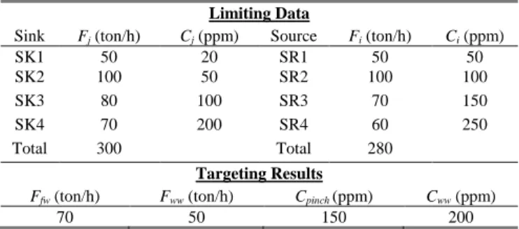
TABLEI: LIMITING DATA AND TARGETING RESULTS FOR EXAMPLE 1
Limiting Data
Sink Fj (ton/h) Cj (ppm) Source Fi (ton/h) Ci (ppm)
SK1 50 20 SR1 50 50
SK2 100 50 SR2 100 100
SK3 80 100 SR3 70 150
SK4 70 200 SR4 60 250
Total 300 Total 280
Targeting Results
Ffw(ton/h) Fww (ton/h) Cpinch(ppm) Cww (ppm)
70 50 150 200
Limiting composite curve can be constructed based on the results of CTA. This is shown in Fig. 1.
Fresh water supply line starts from origin as a pivot and is rotated anticlockwise until touches LCC in the pinch point. Inverse slope of water supply line determines the minimum fresh water requirement. From this graphical representation of CTA, The same targets can be determined.
Fig. 1. LCC and water supply line for example 1.
This demonstrates the hybrid characteristic of Composite Table Algorithm. We have programed this approach using MATLAB. Therefore, it can be used conveniently for any problems, even with large complex industrial processes.
III. FIXED LOAD OPERATIONS
Fixed load water network comprises processes which are quality controlled [17], such as, washing, scrubbing, etc. The main concern for these types of operation is the amount of contaminant mass removal. In this model, each operation has outlet maximum allowable contaminant concentration (Cout) and inlet concentration (Cin) specified by the process constraints. The main assumption is that the water flow rate (F) keeps as constant throughout the process. Then, the fixed amount of mass load (M) will be picked up by water via Eq. (2).
)
(
C
outC
inF
M
(2)TABLEII:LIMITING DATA,DATA CONVERSION, AND TARGETING RESULTS FOR EXAMPLE2
Limiting Data
Process, Pp Δmp(kg/h) Cin (ppm) Cout (ppm) Fp ( ton/h)
1 2 0 100 20
2 5 50 100 100
3 30 50 800 40
4 4 400 800 10
Conversion to FF Model
Sink Fj (ton/h) Cj (ppm) Source Fi (ton/h) Ci (ppm)
P1in 20 0 P1out 20 100
P2in 100 50 P2out 100 100
P3in 40 50 P3out 40 800
P4in 10 400 P4out 10 800
Total 170 Total 170
Targeting Results
Ffw (ton/h) Fww (ton/h) Cpinch(ppm) Cww(ppm)
90 90 100 455.56
To convert the data from fixed load to fixed flow rate model, an inlet stream to any process should be considered as a sink and outlet stream from any operation is treated as a source. Generally, all the inlet streams and outlet streams are regarded as sinks and sources.
Once the integrated network is implemented, 47% of water saving is achievable in this example. Note that fresh water and waste water flow rate are the same because of the fixed load model assumption.
LCC created by MATLAB is illustrated in Fig. 2. The last segment of LCC presents the amount of water loss/gain for total network. The inverse slope of this segment is zero which means no water loss or gain for the network.
Fig. 2. LCC and water supply line for example 2.
IV. COMBINED FF AND FLOPERATIONS
In example 3, the data of examples 1 and 2 are combined to form the new limiting data presented in Table III along with targeting results.
TABLEIII: LIMITING DATA AND TARGETING RESULTS FOR EXAMPLE 3
Limiting Data
Sink Fj(ton/h) Cj(ppm) Source Fi(ton/h) Ci (ppm)
P1in 20 0 P1out 20 100
P2in 100 50 P2out 100 100
P3in 40 50 P3out 40 800
P4in 10 400 P4out 10 800
SK1 50 20 SR1 50 50
SK2 100 50 SR2 100 100
SK3 80 100 SR3 70 150
SK4 70 200 SR4 60 250
Targeting Results
Ffw(ton/h) Fww (ton/h) Cpinch(ppm) Cww (ppm)
155 135 100 377.78
Fig. 3. LCC and water supply line for example 3.
This type of problem was addressed earlier by MRPD method [10]. The consistency of the results from CTA and MRPD is again observed. Please note that the fresh water requirement (155 ton/h) is less than the sum of individual targets for two previous examples (70 + 90 = 160 ton/h). This is because sources in FF model may satisfy inlet stream for FL operation or vice versa. Fig. 3 shows the LCC for this case.
V. MULTIPLE PINCH PROBLEMS
Multiple pinch problem is one of the classes of water network synthesis [18]. The ability of CTA method handling this kind of problem is demonstrated through example 4. FF presentation of limiting data and targeting results are listed in Table IV. Sorin and Bédard [7] using Evolutionary Targeting method initially found only one pinch point at 180 ppm concentration. Later several works [8]-[11] addressed this limitation. In fact, CTA also has the same advantages as WCA, MRPD and WSD methods for multiple pinch problems. Furthermore, its non-iterative and hybrid nature may make it even superior to others. One also can find the relevant limiting composite curve in Fig. 4.
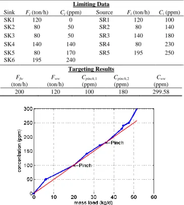
TABLEIV:LIMITING DATA AND TARGETING RESULTS FOR EXAMPLE 4
Limiting Data
Sink Fj (ton/h) Cj (ppm) Source Fi(ton/h) Ci(ppm)
SK1 120 0 SR1 120 100
SK2 80 50 SR2 80 140
SK3 80 50 SR3 140 180
SK4 140 140 SR4 80 230
SK5 80 170 SR5 195 250
SK6 195 240
Targeting Results
Ffw
(ton/h)
Fww
(ton/h)
Cpinch,1
(ppm)
Cpinch,2
(ppm)
Cww
(ppm)
200 120 100 180 299.58
Fig. 4. LCC and water supply line for example 4.
VI. THRESHOLD PROBLEMS
targeting. All limiting data for the following sub-sections are adopted from reference [19].
A. Threshold Problem with Fresh Water Feed and Zero Discharge
Limiting data listed in Table V has been selected for Example 5. Targeting results are also summarized in Table V and illustrated in Fig. 5.
TABLEV:LIMITING DATA AND TARGETING RESULTS FOR EXAMPLE 5
Limiting Data
Sink Fj (ton/h) Cj(ppm) Source Fi(ton/h) Ci(ppm)
SK1 50 20 SR1 20 20
SK2 20 50 SR2 50 100
SK3 100 400 SR3 40 250
Total 170 Total 130
Targeting Results
Ffw (ton/h) Fww (ton/h) Cpinch1 (ppm) Cww(ppm)
34 -26 100 N/A
Fig. 5. Infeasible LCC for example 5.
Dissimilar to forgoing problems, LCC points vertically upward and then left between 100-250 ppm and 250-400 ppm concentration, respectively. This means that for the former concentration interval all sources have been reused/ recycled to process sinks thoroughly and for the latter concentration region the surplus of process sources is available. However, for the first region of LCC (between 0 and 100 ppm), fresh water is needed to fulfill the mass load constraint. The inverse slope of water supply line (shown as red) presents the amount of fresh water requirement. By inspecting the targeting results carefully, it is revealed that this amount of fresh resource is not sufficient for total system due to negative flow rate of waste water. To rectify this infeasibility the absolute amount of waste water flow rate (Fww = 26 ton/h) should be added to fresh water flow rate (Ffw = 34 ton/h). By doing so, the targets have changed to 60 ton/h of fresh water and 0 ton/h of waste water.
To find the pinch point, it is necessary to double check the network with the fresh water source included as one of the process resources. The fourth steps of CTA method for calculating the cumulative mass load is shown in Table VI. Al the values for cumulative mass load are negative which means there is no more pinch point. Hence, this network consumes 60 ton/h of fresh water (64% saving) and generates zero discharge (100% saving) and there is no pinch point. These targets completely match those reported in literature[19].
TABLEVI:FEASIBLE CASCADE TABLE ALGORITHM TO FIND THE PINCH
POINT FOR EXAMPLE 5 Ck
(ppm)
Net.Fk
(t/h)
Δmk
(kg/h)
Cum.Δmk
(kg/h)
0 0
20 -60 -1.2 -1.2
50 -30 -0.9 -2.1
100 -10 -0.5 -2.9
250 -60 -9 -11.6
400 -100 -15 -26.6
(450) 0 (0) (-26.6)
B. Threshold Problem with Waste Disposal Only
The Limiting data, targeting results and LCC for Example 6 are listed in Table VII and shown in Fig. 6.
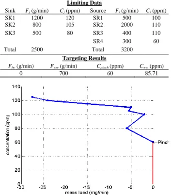
Targeting results have been compared with reference [19] for verification. Nonetheless, there is only one method involved here instead of two complementary methods used by this reference. As targeted, the network has the potential of 100% fresh water saving and reducing waste water by 2500 g/min equated to 78% after reuse/recycling takes place.
TABLEVII:LIMITING DATA AND TARGETING RESULTS FOR EXAMPLE 6
Limiting Data
Sink Fj (g/min) Cj (ppm) Source Fi (g/min) Ci (ppm)
SK1 1200 120 SR1 500 100
SK2 800 105 SR2 2000 110
SK3 500 80 SR3 400 110
SR4 300 60
Total 2500 Total 3200
Targeting Results
Ffw (g/min) Fww (g/min) Cpinch(ppm) Cww (ppm)
0 700 60 85.71
Fig. 6. LCC and water supply line for example 6.
water sources. These special characteristics are unique from this method and cannot easily be found via MRPD or WCA.
C. Threshold Problem with Zero Fresh Water and Zero Discharge
This special case of threshold problems is rare but realistic. Limiting data, targeting results and LCC for this problem (Example 7) are shown in Table VIII and Fig. 7, respectively.
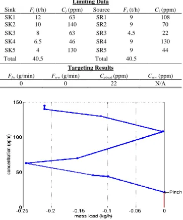
TABLEVIII:LIMITING DATA AND TARGETING RESULTS FOR EXAMPLE 7
Limiting Data
Sink Fj(t/h) Cj(ppm) Source Fi (t/h) Ci (ppm)
SK1 12 63 SR1 9 108
SK2 10 140 SR2 9 70
SK3 8 63 SR3 4.5 22
SK4 6.5 46 SR4 9 130
SK5 4 130 SR5 9 44
Total 40.5 Total 40.5
Targeting Results
Ffw(g/min) Fww(g/min) Cpinch(ppm) Cww(ppm)
0 0 22 N/A
Fig. 7.LCC and water supply line for example 7.
As the characteristics of LCC are the combination of two previous threshold problems, there is no need for further description. For this special case, 100% of fresh water saving and no waste water generating can be achieved. This example seminally was addressed by Hall [20] with the fresh water consumption of 13 ton/h which is a sub-optimal as shown in this work. This problem also has been reported by Foo [19] using MRPD and WCA methods. Here, the applicability of CTA method for this special case is reported. This example is in fact a real case study for organic chemical production.
VII. CONCLUSION
In this work, Composite Table Algorithm is adopted and programmed for variety of problems in water integration. It is proved that this method can successfully find the target both numerically and graphically. Moreover, as this technique has
been programmed by MATLAB, it can be conveniently and trustfully used for any real, complex, and high integrated process industries.
REFERENCES
[1] Y. Wang and R. Smith, “Wastewater minimisation,” Chem. Eng. Sci., vol. 49, pp. 981-1006, 1994.
[2] P. Castro, H. Matos, M. Fernandes, and C. P. Nunes, “Improvements for mass-exchange networks design,” Chem. Eng. Sci., vol. 54, pp. 1649-1665, 1999.
[3] J. G. Mann and Y. A. Liu, Industrial water reuse and wastewater minimization, McGraw-Hill Professional, 1999
[4] Y. Wang and R. Smith, “Wastewater minimization with flowrate constraints,” Chem. Eng. Res. Des., vol. 73, pp. 889-904, 1995. [5] Y. Liu, X. Yuan, and Y. Luo, “Synthesis of water utilization system
using concentration interval analysis method (I) Non-mass-transfer-based operation,” Chin. J. Chem. Eng., vol. 15, pp. 361-368, 2007.
[6] V. R. Dhole, N. Ramchandani, R. A. Tainsh, and M. Wasilewski, “Make your process water pay for itself,” Chem. Eng., vol. 103, 1996. [7] M. Sorin and S. Bédard, “The global pinch point in water reuse networks,” Process Safety Environ. Prot., vol. 77, pp. 305-308, 1999. [8] N. Hallale, “A new graphical targeting method for water
minimisation,” Adv. Environ. Res., vol. 6, pp. 377-390, 2002. [9] M. E. Halwagi, F. Gabriel, and D. Harell, “Rigorous graphical targeting
for resource conservation via material recycle/reuse networks,” Ind. Eng. Chem. Res., vol. 42, pp. 4319-4328, 2003.
[10] R. Prakash and U. V. Shenoy, “Targeting and design of water networks for fixed flowrate and fixed contaminant load operations,” Chem. Eng. Sci., vol. 60, pp. 255-268, 2005.
[11] Z. A. Manan, Y. L. Tan, and D. C. Y. Foo, “Targeting the minimum water flow rate using water cascade analysis technique,” AIChE J., vol. 50, pp. 3169-3183, 2004.
[12] A. M. Almutlaq, V. Kazantzi, and M. M. E. Halwagi, “An algebraic approach to targeting waste discharge and impure fresh usage via material recycle/reuse networks,” Clean Technol. Environ. Policy, vol. 7, pp. 294-305, 2005.
[13] S. Bandyopadhyay, M. D. Ghanekar, and H. K. Pillai, “Process water management,” Ind. Eng. Chem. Res., vol. 45, pp. 5287-5297, 2006. [14] V. Agrawal and U. V. Shenoy, “Unified conceptual approach to
targeting and design of water and hydrogen networks,” AIChE J., vol. 52, pp. 1071-1082, 2006.
[15] C. Deng, X. Feng, and J. Bai, “Graphically based analysis of water system with zero liquid discharge,” Chem. Eng. Res. Des., vol. 86, pp. 165-171, 2008.
[16] C. Deng and X. Feng, “Targeting for Conventional and Property-Based Water Network with Multiple Resources,” Ind. Eng. Chem. Res., 2011. [17] G. T. Polley and H. L. Polley, “Design better water networks,” Chem.
Eng. progress, vol. 96, pp. 47-52, 2000.
[18] D. C. Y. Foo, “State-of-the-art review of pinch analysis techniques for water network synthesis,” Ind. Eng. Chem. Res., vol. 48, pp. 5125-5159, 2009.
[19] D. C. Y. Foo, “Flowrate targeting for threshold problems and plant-wide integration for water network synthesis,” J. Environ. Manage., vol. 88, pp. 253-274, 2008.
[20] S. Hall, “Water and effluent minimisation,” in Symposium papers-institution of chemical engineers north western branch, 1997, pp. 5-8.