124
COMPARATIVE STUDY REGARDING THE OBTAINMENT OF
COORDINATES FOR THE SUPPORT POINTS USING THE TAVERSE
METHOD AND THE METHOD OF THE LEAST SQUARES
GHEORGHE IOSIF University of Craiova
Key words: method of the least squares, traversing, coordinates, radiation
ABSTRACT
A well known truth states that the position (of coordinates) for the new points is determined through several methods: intersections, double radiations, traversing, or the method of the least squares. The new points are being used by specialists in order to create topographical upheavals or cadastral plans. Lately, the great majority of specialists create works for the property right tabulation over small surfaces. Considering the development of the GNSS technology, two GNSS receptor points are determined for the support points from which the traversing is being drawn. Theoretically traversing is not the best method. It is recommended to use the method of the least squares since this takes into account all the measurements conducted. This statement will be demonstrated in this study.
GENERAL CONSIDERATIONS
Lately, the topographic instruments have evolved. Ever since the emergence of the total stations and the GPS technology, subsequently turned into GNSS, performances have been registered that were difficult to reach otherwise.
Thus, we can now talk about millimeter precisions, and millimeter errors. If we look at the data shown by the reports after the processing of the GNSS data, we can say that the position is given with a precision centimeter level, for the least. From the perspective of the used devices these precisions are credible, considering their performances. From the perspective of data processing however, it is questionable whether the precisions are real, and weather the coordinates are the closest possible to the real value.
This is not always the case, we start from the GNSS receptors that produce very good positions in the system WGS84, but which need to be transformed in a plane projection system, the Stenographic 1970 system.
Luckily, today we have ROMPOS and TRANSDAT, which secure a millimeter precision, not a centimeter one but one that secures uniformity. It is not the purpose of this work to study the way in which the positions are obtained using the technology GNSS, so we will not go into further detail. We will remain at the level of studying the traversing method versus the method of the least squares.
In general, specialists in cadaster and topography are currently handling works at a smaller scale, mostly field tabulation documentations for small land owners. For the topographic upheavals they need a support network from which the detail points radiate.
The support network is translated into:
- traversing from the old points existing in the area;
- intersections from which a traversing starts towards the interest area:
- two points are being determined with the help of the GNSS technology from a traversing in the interest area is being conducted.
125
COMPENSATING THE MEASURES THROUGH THE METHOD OF THE LEAST SQUARES
The method of the least squares is very well known, hence this is not the case to repeat all its formulas. Currently, due to the calculation system development, the Gauss method is no longer in use, instead, the conditional measurements and the matrix treatment are being used. Each measurement gives an equation, each new point gives two unknown (coordinates x and coordinate y). The number of measurement (equations) has to be larger than the number of unknown factors in order to obtain the most probable value of the coordinate as close as possible to the real value. Equations are of two or three kinds (on directions, on distances, and on GNSS determinations). In the study cases illustrated only two types of equations have been considered: based on directions, and based on distances. The general case used in processing the data is the method of the least squares, indirect measurements in which each measurement (on direction and on distance) gives out an equation. The equations are different for the two types of measurements, but have the unknown factor in common, respectively the coordinates x and y of the new points.
For both methods to obtain the position it is considered that the distance has been correctly reduced to the 1970 Stenographic projection plan.
Having the correction equations based on directions, distances and difference of coordinates, the following matrix relations can be written:
(2.1)
(2.2)
(2.3)
in which:
- is the correction matrix;
- is the matrix of the correction factor; - is the matrix of the unknown factor;
- is the matrix of weighing factor.
The equations for distances have the following form:
(2.4)
The free term is calculated as follows:
126 And
(2.6)
(2.7)
The correction equations for directions have the following form:
(2.8)
(2.9)
(2.10)
(2.11)
For each determined new point the precisions with which it has been calculated can be obtained. The forms are the following:
, cu j=1,2 ...n (2.12)
Quotients Qij are extracted from the main transverse of the matrix opposite to the
normal system (matrix N-1 )
DETERMINING THE COORDINATES BY USING THE TRASVERSING METHOD
The traversing method is a procedure largely used by the cadaster and geodesy specialists for areas with a small surface. Practically, it starts from a point with known coordinates, on top of which the total station is positioned, with another aimed point which also has known coordinates. From the stationary point, the next point of the traversing is aimed at, also a point that has known coordinates. The next point of the traversing is aimed at from the stationary point, correlated to the previously aimed point, thus the departure orientation can be determined. Also the forth and back distances can be measured (from the point with known coordinates to the new point, and then backwards).
127
Practically, the coordinates are determined from one close up to another and are finally closed on an unknown point. The coordinates transmitted through the traversing should be close to the ones from the inventory, considering the precision of the old network and the errors accumulated in the traversing.
The general formulas of determination are:
(3.1)
The coordinates are being determined from one close up to another, finally reaching a point for known coordinates (the closing point). Between the sent coordinates and the coordinates already existing there is a difference that is called error of unclosing the traversing.
(3.2)
Total linear error:
(3.3)
This error must not overcome the imposed tolerance. The tolerance is given by the precision of the device with which is being worked. If the errors are within the tolerance limit, unitary corrections are being calculated:
(3.4)
In which D is the sum of the distances reduced to the 1970 Stenographic projection plan.
(3.5)
The unitary correction is applied to each Δx and Δy according to distance. After applying the corrections, the coordinates are being retransmitted from one close up to another and
. Each point of the traversing will have new coordinates, corrected according to the traversing and the closing on the traversing.
CASE STUDY
A geodetic network has been created for the thickening whose beneficiary was the local Timis Waters Bazin Administration (Figure xx1). Within the network distances and directions have been determined. There have been 9 points with known coordinates and the new determined points have been 10. The number of equations was 89, enough to apply the method of the least squares and the indirect measures. The network has been compensated and the result have been the precisions presented in the table 4.1.
128
ends (Figure xx2). We have calculated the coordinates with the known formulas and we have obtained the provisory positions. The traversing has been compensated and the unclosing has been -6,19 centimeters on the X axe, and 52,98 centimeters on the Y axe, respectively 53,34 centimeters total unclosing. The total length of the traversing has been of 5984,45 meters and the number of stations of 12. The starting point has been the point "La Gomila" and the closing have been on the point "Biled Nord". Both points are part of the national geodetic network .
Table 1
Compensated through the method of the least squares and the obtained precisions
Name of the point
X
compensated
precision x
Y
compensatated precision y
Total precision
[m] [mm] [m] [mm] [mm]
BIS_SIRBEA 489381.005 0 193158.665 0 0
CA_SANDRA 499303.616 0 182951.287 0 0
BIS_BILED 495532.999 0 186890.594 0 0
BIS_SATCHINEZ 501354.193 0 192865.766 0 0
CAT_SATCHINEZ 500861.438 0 193459.266 0 0
LA_GOMILA 500021.708 0 189945.826 0 0
BIS_HODONI 496756.611 0 196534.092 0 0
BILED_NORD 496829.017 0 188278.994 0 0
BECIC 488937.319 0 193280.931 0 0
B33 499415.774 20 189689.407 23 30
B31 499875.812 20 190528.606 16 26
B30 500117.425 23 190729.652 18 29
B32 499445.179 22 190228.591 23 32
B34 499154.698 28 189222.829 30 41
B35 498864.445 32 188690.549 34 47
B36 498225.579 32 188442.562 37 49
B37 497616.381 27 188817.25 33 42
B38 497015.843 17 188654.847 15 22
B39 496808.699 18 188714.993 14 23
Medium error for determining a point: 25 mm
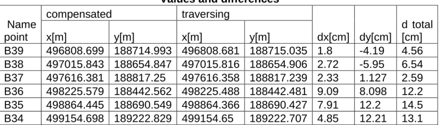
After obtaining the coordinated in the two variants we have created the table (Table 4.2) with the values of the positions and the differences between the two variants.
Table 2.
Values and differences
Name point
compensated traversing
dx[cm]
dy[cm]
d total [cm]
x[m] y[m] x[m] y[m]
129
B33 499415.774 189689.407 499415.748 189689.287 2.64 11.97 12.3 B32 499445.179 190228.591 499445.162 190228.505 1.75 8.596 8.77 B31 499875.812 190528.606 499875.796 190528.539 1.57 6.723 6.9 B30 500117.425 190729.652 500117.416 190729.603 0.92 4.927 5.01
CONCLUSIONS
The case presented is an example proving there are large differences influencing the coordinates of the radiated points between the coordinated determined by the traversing and those determined by the method of the least squares, the indirect measurements.
The radiated points often represent coins of property defining edges. If two properties are being measured by two different specialists, and they will obtain those coordinates in a different way using another method of calculation, subsequently also the coordinates of the common points will be substantially different. We are also not mentioning the different techniques used to measure the land, which can also lead to errors of positioning.
In general, authorized cadaster specialists use the method of traversing because it is easier to calculate. This is wrong since currently, with the help of evolved computers, we can work the data very easy. Let us take for instance the Excel program, delivered along with the computer. This program allows us to work with needed matrixes regarding the least squares method. We have to know that a not very large network is being developed usually, this only for a certain property. Further more, the calculation will be very simple.
From the table 4.2, we can see that the differences of coordinates are smaller at the heads and bigger in the middle, as it was normal as the constriction is done at the heads.
It can be noticed that the total error in the middle is over 13 centimeters.
The conclusion is that it will be necessary to obtain the final coordinates using the methods of the least squares, which offers a value much closer to the real one.
BIBLIOGRAPHY
1. Ghiţău Dumitru – Geodezie şi Gravimetrie geodezică, Editura didactică ţi pedagogică, Bucureşti 1983
2. Moldoveanu Constantin – Geodezie. Noţiuni de geodezie fizică şi elipsoidală,
poziţionare, Editura MATRIXRom 2002