Estimation of the Parameters of the New Weibull-Pareto Distribution Using Ranked Set Sampling

(1)

ESTIMATION OF THE PARAMETERS OF THE NEW

WEIBULL-PARETO DISTRIBUTION USING RANKED SET

SAMPLING

Monjed H. Samuh1

Department of Applied Mathematics & Physics, Palestine Polytechnic University, Hebron, Palestine Amer I. Al-Omari

Department of Mathematics, Al al-Bayt University, Al-Mafraq, Jordan Nursel Koyuncu

Department of Statistics, Hacettepe University, Ankara, Turkey

1. INTRODUCTION

1.1. Ranked set sampling

McIntyre (1952) introduced the concept of ranked set sampling (RSS) as a new sampling scheme for data collection. Due to its importance for a variety of applications in statis-tics, it is republished in McIntyre (2005) to estimate the mean of Australian pasture and forage yields. As claimed by McIntyre (1952, 2005), the mean of the RSS is an unbiased estimator of the population mean. Also, the variance of the RSS mean is smaller than that of the simple random sampling (SRS) with equal number of measurement elements. This sampling scheme is useful when it is difficult to measure large number of elements but visually (without inspection) ranking some of them is easier. For example, in McIn-tyre’s experiment the yields of pasture plots can be assessed without the actual laborious process of weighing and mowing the hay for a lots of plots. Moreover, the RSS scheme is also highly applicable in instances where measuring a variable of interest is difficult and risky to measure. For example, in studying some diseases such as the yellowing of the body of an infant, one of the main steps is to measure the bilirubin level of the infant by taking their blood samples. However, it is risky and excruciating to take the blood samples. It is rather easy to rank the babies and take the measurement of the bilirubin level on their urine samples (Paul and Thomas, 2017).

The RSS consists of the following steps:

(2)

1. randomly selectmsets each of sizemelements from the population under study (typicallymis in the range 2 to 5);

2. the elements for each set in Step (1) are ranked visually or by any negligible cost method that does not require actual measurements;

3. select and quantify theith_{minimum from the}_ith_set,_i₌_{1, 2, ...,}_m_{, to get a new} set of sizem, which is called the ranked set sample;

4. repeat Steps (1)-(3)htimes (cycles) until obtaining a sample of sizen=mh. Theith_{data point (measured unit) acquired in the} _jth_{cycle is denoted by}_Y

j i =Xj(i),

i =1, 2, . . . ,m, and j=1, 2, . . . ,h. This version of RSS is a balanced RSS, in the sense that in each cycle the number of data points is fixed. The following matrices clarify the procedure of RSS.

Step 1: 

   

X11 X12 · · · X1m X21 X22 · · · X2m

. . .

. .

. ... ...

X_m₁ X_m₂ · · · X_mm



   

Step 2: 

    

X1(1) X1(2) · · · X1(m)

X2(1) X2(2) · · · X2(m)

. . .

. .

. ... ...

Xm(1) Xm(2) · · · Xm(m) 

    

Step 3:{X1(1),X2(2), . . . ,Xm(m)} Step 4: 

   

Y11 Y12 · · · Y1m Y21 Y22 · · · Y2m

. . .

. .

. ... ...

Yh1 Yh2 · · · Yh m



   

Note that althoughh×m2elements are sampled, onlyh×mof them are selected for measurement. In case of perfect ranking (no error was made in the ranking mecha-nism) the measured elements are called theorder statisticsand they are not ordered (see Navarroet al., 2007, for some examples where order statistics are not ordered). In case of imperfect ranking the measured elements are called thejudgment order statistics.

Dell and Clutter (1972) and Takahasi and Wakimoto (1968) explained the mathemat-ical theory behind the claims of McIntyre (1952, 2005) by showing that the efficiency of the RSS mean with respect to SRS, defined by the ratio of the variances of the two sample means, is bounded by 1 and(m+1)/2. Moreover, Dell and Clutter (1972) also proved that the RSS mean is at least as efficient as the SRS mean even when there are ranking errors. For more about RSS see Al-Saleh and Samuh (2008), Samuh and Al-Saleh (2011), Al-Nasser and Al-Omari (2015), Al-Omari and Haq (2015), Al-Omari (2016), Amro and Samuh (2017), and Samuh (2017).

(3)

by Khamnei and Abusaleh (2017). Esemen and Gürler (2017) investigated the method of maximum likelihood of the shape and scale parameters of the generalized Rayleigh distribution within the context of RSS. For more results and references, see Lamet al. (1994), Bhoj and Ahsanullah (1996), Chacko and Thomas (2008), Al-Saleh and Diab (2009), Sarikavanijet al.(2014), and Samuh and Qtait (2015).

The purpose of this paper is to study the maximum likelihood estimation of the parameters concerning the new Weibull-Pareto distribution within the context of SRS, RSS, median RSS (MRSS), and extreme RSS (ERSS).

The organization of the paper is the following. The new Weibull-Pareto distribution is introduced in Section 2. Maximum likelihood estimation and Fisher information are discussed in Section 3. Interval estimates for the parameters are constructed in Section 4. A simulation study is carried out in Section 5. A real data application is presented in Section 6. Finally, Section 7 concludes the paper.

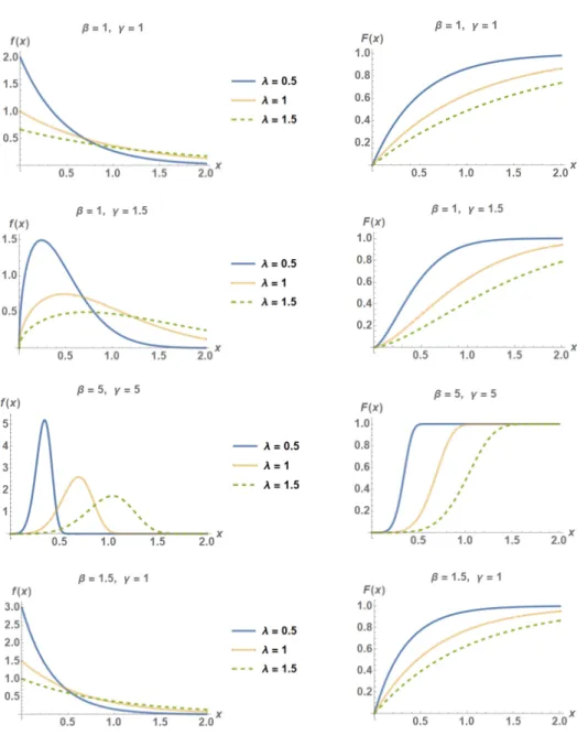
2. THE NEWWEIBULL-PARETO DISTRIBUTION

The new Weibull-Pareto (NWP) distribution is defined by Nasiru and Luguterah (2015) as a generalization of the Pareto distribution. It is of great interest and is popularly used in analyzing lifetime data. For example, it is used by Nasiru and Luguterah (2015) to model the exceedances of flood peaks (inm3_/_s_{) of the Wheaton River near Carcross in} Yukon Territory, Canada. Aljarrahet al.(2015) used the NWP distribution to model the remission times (in months) of a random sample of 128 bladder cancer patients.

The probability density function (pdf) of the NWP distribution, with shape param-eterγ and scale parametersβandλ, is given by

f(x;β,γ,λ) =βγ λ

x λ

γ−1 e−β(xλ)

γ

, x>0,β,γ,λ >0. (1)

The corresponding cumulative distribution function (cdf) is given by F(x;β,γ,λ) =1−e−β(xλ)

γ

. (2)

The mean of the NWP distribution is

µ=E(X) =λβ−1/γΓ

1+ 1 γ

(3)

with variance defined as

σ2₌_Var₍_X_{) =}_λ2_β−2/γ

Γ

_γ₊ 2 γ

−Γ

1+ 1

γ 2

(4)

(5)

3. MAXIMUM LIKELIHOOD ESTIMATION ANDFISHER INFORMATION

In this section, the maximum likelihood estimation of the shape parameterγand scale parametersβandλfor NWP distribution based on SRS, RSS, MRSS, and ERSS is in-vestigated.

3.1. Using SRS

SupposeX₁,X₂, . . . ,X_nbe a random sample of sizenselected from the NWP distribution f(x;β,γ,λ), where the values ofβ,γ, andλare unknown. The likelihood function L_SRS(β,γ,λ)is given by

L_SRS(β,γ,λ) =Yn

i=1

f(x_i;β,γ,λ)

=βnγn

Qn

i=1

xi λ

_γ

e−βPni=1(xiλ)γ

Qn i=1xi

. (5)

Thus, the log likelihood functionl_SRS(β,γ,λ)is l_SRS(β,γ,λ) =logL_SRS(β,γ,λ)

=nlog(β) +nlog(γ)−nγlog(λ) +γ

n

X

i=1 log(x_i)

−βλ−γ

_n X

i=1 x_iγ

− n

X

i=1

log(x_i). (6)

Differentiating the log likelihood function with respect toβ,γ, andλ, respectively, yields

∂l_SRS(β,γ,λ)

∂ β =

n β−λ−γ

_n X

i=1 x_iγ

, (7)

∂ γ =

n

γ −nlog(λ) +

n

X

i=1

log(x_i)−βλ−γ

_n X

i=1

x_iγlog(x_i)

+βλ−γ_log₍_λ₎

_n X

i=1 x_iγ

, (8)

and

∂ λ =βγλ−γ−1

n

X

i=1

x_iγ−γn

(6)

The MLE ofβas a function ofγ andλ, say ˆβ(γ,λ), can be obtained as

ˆ

β(γ,λ) =_Pn_nλγ

i=1x

γ i

, (10)

and the MLE ofλas a function ofβandγ, say ˆλ(β,γ), can be obtained as

ˆ λ(β,γ) =

_βPn i=1x

γ i

n

1/γ

. (11)

The MLE ofγcannot be written in explicit form. So, estimates forγcan be obtained by using numerical methods. Themle2function in thebbmlepackage in R (R Core Team, 2018) is used.

The Fisher information (FI) number is used to measure the amount of information that an observable sample carries about the parameter(s). The FI number for the param-eterθis defined as

F I(θ) =−E

∂2_log_L₍_θ₎ ∂ θ2

.

For a random sampleX₁,X₂, . . . ,X_nfrom the NWP distribution, the FI numbers of β,γ, andλare, respectively, given by

F I_SRS(β) =−E ∂2_l

SRS(β,γ,λ)

∂ β2

= n

β2, (12)

F I_SRS(λ) =−E ∂2_l

SRS(β,γ,λ)

∂ λ2

= nγ2

λ2 , (13)

F I_SRS(γ) =−E ∂2_l

SRS(β,γ,λ)

∂ γ2

=n 6 log(β)(log(β) +2C−2) +6(C−1)

2₊_π2

6γ2 , (14)

whereC=−Γ0₍₁₎_{is the Euler’s constant. The observed FI numbers are evaluated at the}

maximum likelihood estimates.

3.2. Using RSS

(7)

1, 2, . . . ,h, is the same as the distribution of theith_{order statistic of the random sample} X₁,X₂, . . . ,X_m, that is

f_Y

j i(y) =fX(i)(y) =

m!

(i−1)!(m−i)!f(y)(F(y))

i−1₍₁₋_F₍_y₎₎m−i

= m!βγλ−γyγ−

1 ₁₋_eβλ−γ₍₋_yγ₎i

e−βλ−γ₍_m₋_i₎_yγ (i−1)!(m−i)! eβλ−γ_yγ

−1 . (15)

The likelihood function of RSS{Y_{j i},j=1, 2, . . . ,h,i=1, 2, . . . ,m}is given by

L_RSS(β,γ,λ) =

m

Y

i=1

h

Y

j=1 f_Y

j i(yj i)

=Ym

i=1

h

Y

j=1

m!βγλ−γ_yγ−1

j i

1−eβλ−γ

−yγ_{j i}i_e−βλ−γ₍_m₋_i₎_yγ

j i

(i−1)!(m−i)!eβλ−γyγj i₋₁

= β

mh_γmh_λγ(−mh)Qm

i=1 Qh

j=1

1−e−βλ−γyγi ji

Qm

i=1 Qh

j=1

eβλ−γyi jγ₋₁

× m

Y

i=1

h

Y

j=1

yγ_{i j}−1e−βλ−γPim=1

Ph

j=1(m−i)yγi j_. ₍₁₆₎

Thus, the log likelihood function is

lRSS(β,γ,λ) =mhlog(β)−γmhlog(λ) +mhlog(γ)

−

m X

i=1

h X

j=1

logeβλ−γyγj i₋₁

+

m X

i=1

h X

j=1

(γ−1)log(yj i)

+

m X

i=1

h X

j=1

ilog1−e−βλ−γyγj i

−βλ−γ Xm i=1

h X

j=1

(m−i)yγ_{j i}

!

. (17)

Differentiatingl_RSS(β,γ,λ)with respect toβ,γ, andλ, respectively, we get

∂l_RSS(β,γ,λ)

∂ β =

mh

β −

m

X

i=1

h

X

j=1 λ−γ_yγ

j i

eβλ−γyγj i₋_i

eβλ−γyγj i₋₁ −λ−γ

m

X

i=1

h

X

j=1

(8)

∂l_RSS(β,γ,λ)

∂ γ =

mh

γ −mhlog(λ) +

m

X

i=1

h

X

j=1 log(y_{j i})

+βλ−γXm

i=1

h

X

j=1

(m−i)yγ_{j i}(log(λ)−log(y_{j i}))

+Xm

i=1

h

X

j=1

βλ−γ_yγ

j i(log(λ)−log(yj i))

eβλ−γyγj i₋₁

, (19)

∂l_RSS(β,γ,λ)

∂ λ =−

γmh

λ +βγλ−γ− 1Xm

i=1

h

X

j=1

(m−i)yγ_{j i}

+Xm

i=1

h

X

j=1

βγλ−γ−1_yγ

j i

eβλ−γyγj i₋₁

. (20)

The solutions of these equations give the MLEs of the parametersβ,γandλ. How-ever, the solutions are not in closed forms, and hence the estimates forβ,γandλ, can be obtained by solving the equations numerically. Let us denote them by ˆβ_RSS, ˆγ_RSS and ˆλ_RSS, respectively.

3.3. Using ERSS

ERSS was proposed by Samawiet al.(1996). The procedure of the ERSS is described as follows.

1. Randomly selectmsets of sizemelements each from the study population. These may be denoted as set 1={Z₁₁∗,Z₁₂∗, . . . ,Z₁∗_m}, set 2={Z₂₁∗,Z₂₂∗, . . . ,Z₂∗_m}, and so on till the last set, setm={Z_m∗₁,Z_m∗₂, . . . , Z_mm∗ }. It is assumed that the largest and lowest elements in each set can be determined virtually or by any negligible cost method. This is of course, a simple and practical approach.

2. Ifmis even, measure the lowest ranked element in set 1. Repeat this procedure for set 2 till set(m/2). Represent the measured elements as Z₁,Z₂, . . . ,Z₍_m_/₂₎. Furthermore, measure the largest ranked element in set(m/2+1). Repeat this procedure for set(m/2+2)till the last set, setm. Represent the measured elements asZ₍_m_/₂₊₁₎,Z₍_m_/₂₊₂₎, . . . ,Z_m.

(9)

procedure for set((m+3)/2)till set(m−1). Represent the measured elements as Z₍₍_m₊₁₎_/₂₎,Z₍₍_m₊₃₎_/₂₎, . . . ,Z₍_m₋₁₎. Elements in the last set can be measured in two different ways:

• select the average of the measures of the lowest and the largest ranked ele-ments, or

• measure the median ranked element, sayZ_m. In this paper, we consider this way. The acquired sample,{Z₁,Z₂, . . . ,Z_m}, is called an ERSS of sizem.

4. Independently repeat the stepshcycles, if needed, to acquire an ERSS of sizen=

h×m.

To this end, the ERSS scheme produces a data set as follows

Z={Z_{j i}}=



   

Z₁₁ Z₁₂ · · · Z₁_m Z₂₁ Z₂₂ · · · Z₂_m

..

. ... ... ... Z_h₁ Z_h₂ · · · Z_{h m}



    .

Accordingly, the likelihood function of the parameters depends on whethermis odd or even. Let us denote the pdf of theith_{order statistic by}_g

i(zj i). For even set sizem, the

likelihood function of ERSS{Z_{j i},j=1, 2, . . . ,h,i=1, 2, . . . ,m}is given by

LE RSS_e(β,γ,λ) =

m

2 Y

i=1

h Y

j=1 g1(zj i)

m Y

i=m

2+1 h Y

j=1 gm(zj i)

= m

2 Y

i=1

h Y

j=1

mβγλ−γ_zγ−1

j i e −mβλ−γ_zγ

j i

×

m Y

i=m

2+1 h Y

j=1

j i

1−e−βλ−γzγj i

m

eβλ−γzγj i₋₁

= mβγλ−γh mYm

i=1

h Y

j=1 zγ_{j i}−1

m

2 Y

i=1

h Y

j=1

e−mβλ−γzγj i

×

m Y

i=m

2+1 h Y

j=1

m

(10)

For odd set sizem, the likelihood function is

LE RSS_o(β,γ,λ) =

m−1 2 Y

i=1

h Y

j=1 g1(zj i)

m−1

Y

i=m+1 2

h Y

j=1 gm(zj i)

m Y

i=m h Y

j=1 gm+1

2 (zj i)

= m−1

2 Y

i=1

h Y

j=1

j i e −mβλ−γ_zγ

j i

×

m−1

Y

i=m+1 2

h Y

j=1

j i

m

×

m Y

i=m h Y

j=1

βγm!λ−γ_zγ−1

j i e

−1₂β(m−1)λ−γzγ

j i

1−eβλ−γ

−zγ_{j i}

m+1 2

Γ_m₊₁

2

= m!hmh(m−1)(βγλ−γ)

h m

Γ_m₊₁

2

2h

m Y

i=1

h Y

j=1 zγ_{j i}−1

m−1 2 Y

i=1

h Y

j=1

e−mβλ−γzγj i

×

m−1

Y

i=m+1 2

h Y

j=1

m

×

m Y

i=m h Y

j=1

e−12β(m−1)λ−γz γ

j i

1−eβλ−γ

−zγ_{j i}

m+1

2

. (22)

As there are no closed form of the MLEs under even and odd set sizem, the MLEs ˆ

βE RSS, ˆγE RSSand ˆλE RSSare obtained numerically.

3.4. Using MRSS

MRSS was proposed by Muttlak (1997). The procedure of the MRSS is described as follows.

1. Randomly selectmrandom samples, each of sizemelements, from a target pop-ulation.

2. The elements of each random sample in Step 1 are ranked visually with regards to the variable of interest.

(11)

from the firstm/2 samples the(m/2)-th smallest rank element and from the sec-ondm/2 samples the[(m+2)/2]-th smallest rank element. This step yieldsm sample elements which is the median RSS.

4. Repeat Steps 1-3hcycles until obtaining a sample of sizen=mh.

SupposeX₁,X₂, . . . ,X_n be a random sample of sizen selected from the NWP dis-tribution f(x;β,γ,λ). LetV ={V_{j i},j =1, 2, . . . ,h,i =1, 2, . . . ,m}be a MRSS; that is

V_{j i}=

  

 

X₍m+1

2 ) ifmis odd ,i=1, . . . ,m&j=1, . . . ,h

X₍m

2) ifmis even ,i=1, . . . ,

m

2 &j=1, . . . ,h X₍m+2

2 ) ifmis even ,i=

m+2

2 , . . . ,m&j=1, . . . ,h. The pdf ofV_{j i}is

g_V

j i(v) =

      

gm+1

2 (vj i) =fX(m+1 2 )

(v) ifmis odd ,i=1, . . . ,m&j=1, . . . ,h gm

2(vj i) =fX(m

2)

(v) ifmis even ,i=1, . . . ,m₂ &j=1, . . . ,h gm+2

2 (vj i) =fX(m+2 2 )

(v) ifmis even ,i=m₂+2, . . . ,m&j=1, . . . ,h.

The likelihood function of the parameters depends on whethermis odd or even. For even set sizem, the likelihood function of MRSS{V_{j i}, j=1, 2, . . . ,h,i=1, 2, . . . ,m}is given by

LM RSS_e(β,γ,λ) =

m

2 Y

i=1

h Y

j=1 gm

2(vj i) m Y

i=m

2+1 h Y

j=1 gm+2

2 (vj i)

= m

2 Y

i=1

h Y

j=1

βγm!λ−γ_vγ−1

j i e

−1₂βmλ−γvγ

j i

1−eβλ−γ

−vγ_{j i}m/2

Γ m

2 +1

Γ m

2

eβλ−γvγj i₋₁

×

m Y

i=m

2+1 h Y

j=1

j i e

−1₂βmλ−γ_vγ

j i

1−eβλ−γ

−vγ_{j i}m/2

Γ m

2 +1

Γ m 2 =

m!βγλ−γ

Γ m

2 +1

Γ m

2

h m m/2

Y

i=1

h Y

j=1

1

×

m Y

i=1

h Y

j=1

e−12βmλ−γvγj i

1−eβλ−γ

−vγ_{j i}m/2

(12)

For odd set sizem, the likelihood function is

LM RSS_o(β,γ,λ) = m Y

i=1

h Y

j=1 gm+1

2 (vj i)

=

m Y

i=1

h Y

j=1

j i e

−1₂β(m−1)λ−γvγ

j i

1−eβλ−γ

−vγ_{j i}

m+1 2

Γ_m₊₁

2

=





m!βγλ−γ Γ_m₊₁

2

2 

 h m

m Y

i=1

h Y

j=1

vγ_{j i}−1e−12β(m−1)λ−γvγj i

1−eβλ−γ

−vγ_{j i}

m+1 2

. (24)

Again, there are no closed form of the MLEs under even and odd set size m, the MLEs ˆβ_{M RSS}, ˆγ_{M RSS}and ˆλ_{M RSS}are obtained numerically.

The comparison between different estimators of a specific parameterθcan be done using the asymptotic efficiency (see Basu, 1956). The asymptotic efficiency of ˆθ₁with respect to ˆθ2for estimatingθis defined by

Aeff(θˆ₁; ˆθ₂) = lim

n→∞eff(

ˆ θ1; ˆθ2) =

F I₁(θ) F I₂(θ).

Since the FI numbers ofβ,γ, andλcannot be obtained in closed form under RSS, ERSS, and MRSS, their values will be obtained through a simulation study.

4. INTERVAL ESTIMATES

LetX₁, . . . ,X_n be a random sample from f(x;θ), whereθis an unknown quantity. A confidence interval for the parameterθ, with confidence coefficient 1−α, is an interval

with random endpoints[L(X₁, . . . ,X_n),U(X₁, . . . ,X_n)]. It is given by P(L(X₁, . . . ,X_n)≤θ≤U(X₁, . . . ,X_n)) =1−α.

The interval[L(X₁, . . . ,X_n),U(X₁, . . . ,X_n)]is the well-known 100(1−α)% confidence interval forθ. Moreover, let ˆθbe the MLE ofθ. It is well known that, under some mild regularity conditions (see Davison, 2008, p. 118), the MLE has the following properties:

1. ˆθis asymptotically consistent; 2. ˆθis asymptotically unbiased;

3. the sampling distribution of ˆθis asymptotically normal with its variance obtained from the inverse Fisher information number of sample size 1 at the unknown parameterθ; that is, ˆθM LE→N θ,F I−1(θ)

(13)

Accordingly, the approximate 100(1−α)% confidence limits for ˆθofθcan be con-structed as

P 

−zα

2 ≤

ˆ θ−θ

q F I−1(θˆ)

≤zα 2



=1−α,

wherez_αis theαthupper percentile of the standard normal distribution.

Therefore, the approximate 100(1−α)% confidence limits for the parametersβ,γ andλof the NWP distribution are given, respectively, by

P

ˆ β−zα

2

Ç

F I−1₍_βˆ₎_≤_β_≤_βˆ₊_z_α

2

Ç

F I−1₍_βˆ₎

=1−α,

P

ˆ γ−zα

2

Ç

F I−1₍_γˆ₎_≤_γ_≤_γ_ˆ₊_z_α

2

Ç F I−1₍_γˆ₎

=1−α,

P

ˆ λ−zα

2

Ç

F I−1(λˆ)_≤λ_≤λˆ+_zα 2

Ç F I−1(λˆ)

=1−α.

5. SIMULATION STUDY

To investigate the properties of the proposed MLEs of the parametersβ,γ andλof the NWP distribution a simulation study is conducted. Monte Carlo simulation is applied for different sample sizes, m ={4, 5}and h ={10, 50, 100}, for the parameter values

(β=1.5,γ =1,λ=0.5)and(β=0.5,γ =2,λ=1.5). Biases and MSEs of the MLEs ofβ,γandλare computed over 10000 replications under SRS, RSS, ERSS, and MRSS, where

Bias(θˆ) =E(θˆ−θ), and

MSE(θˆ) =E(θˆ−θ)2.

(14)

(15)

T ABLE 2 The bias, MSE, and ef ficiency values of estimating the par ame ter s ( β = 0.5, γ = 2, λ = 1.5 )under SRS, RSS, ERSS, and MRSS. β = 0.5 γ = 2 λ = 1.5 n = m × h Sam pling Bias (

ˆ_β)

MSE

(

ˆ_β)

Ef f Bias ( ˆ γ ) MSE ( ˆ γ ) Ef f Bias (

ˆ_λ)

MSE

(

ˆ_λ)

(16)

TABLE 3

A95%asymptotic confidence interval for (β=1.5,γ=1,λ=0.5) under SRS, RSS, ERSS, and MRSS.

SRS RSS

Parameter Interval Width Interval Width

β (1.426, 1.685) 0.259 (1.444, 1.643) 0.198

γ (0.936, 1.071) 0.135 (0.950, 1.054) 0.104

λ (0.466, 0.570) 0.104 (0.477, 0.552) 0.075

ERSS MRSS

β (1.443, 1.646) 0.204 (1.442, 1.650) 0.208

γ (0.953, 1.050) 0.097 (0.938, 1.068) 0.130

λ (0.477, 0.552) 0.076 (0.473, 0.556) 0.083

TABLE 4

A95%asymptotic confidence interval for (β=0.5,γ=2,λ=1.5) under SRS, RSS, ERSS, and MRSS.

SRS RSS

β (0.445, 0.617) 0.173 (0.464, 0.585) 0.122

γ (1.871, 2.141) 0.270 (1.898, 2.110) 0.213

λ (1.440, 1.652) 0.212 (1.452, 1.622) 0.170

ERSS MRSS

β (0.460, 0.593) 0.133 (0.467, 0.579) 0.112

γ (1.904, 2.102) 0.198 (1.875, 2.135) 0.260

(17)

6. REAL DATA APPLICATION

In this section, a real-life data set is analyzed for the purpose of illustration to show the usefulness of the RSS, MRSS, and ERSS schemes in reducing the MSEs of the estimators comparing with the traditional SRS scheme. Data set includes the 72 exceedances of flood peaks (inm3_/_s_{) of the Wheaton River near Carcross in Yukon Territory, Canada,} for the year 1958-1984, rounded to one decimal place (Choulakian and Stephens, 2001). The observations are given in Table 5.

TABLE 5

Exceedances (in m3_/_{s) of Wheaton river flood data.}

1.7 2.2 14.4 1.1 0.4 20.6 5.3 0.7 1.4 18.7 8.5 25.5

11.6 14.1 22.1 1.1 0.6 2.2 39.0 0.3 15.0 11.0 7.3 22.9

0.9 1.7 7.0 20.1 0.4 2.8 14.1 9.9 5.6 30.8 13.3 4.2

25.5 3.4 11.9 21.5 1.5 2.5 27.4 1.0 27.1 20.2 16.8 5.3

1.9 10.4 13.0 10.7 12.0 30.0 9.3 3.6 2.5 27.6 14.4 36.4

1.7 2.7 37.6 64.0 1.7 9.7 0.1 27.5 1.1 2.5 0.6 27.0

To assess whether this data set is well-modeled by a NWP distribution, Kolmogorov-Smirnov test is applied. The MLEs of the parametersβ,γ,λ and the p-value of the Kolmogorov-Smirnov test are 0.238, 0.883, 2.24 and 0.3526, respectively. The p-value is not significant, and thus, the data can be modeled by the NWP distribution.

For purposes of comparison, a SRS of size 15 is drawn from this data set, and in RSS and its modificationsm=3 andh=5 are chosen. The NWP distribution is fitted to each of these samples (SRS, RSS, MRSS, and ERSS). For each of them, the MLEs, the Akaike information criterion (AIC), and Bayesian information criterion (BIC) are evaluated and the results are reported in Table 6. According to the values of AIC and BIC, data obtained by RSS is the best data fitted by the NWP distribution.

TABLE 6

The MLEs, -2LL, AIC, and BIC values for Exceedances of Wheaton river flood data under SRS, RSS, MRSS, and ERSS.

Sampling Parameter Estimates(_{β, ˆ}ˆ _γ_{, ˆ}_λ) _-2LL _AIC _BIC

SRS (0.199, 0.886, 2.487) -56.629 119.258 121.382

RSS (0.311, 0.776, 2.334) -51.498 108.996 111.120

MRSS (0.064, 1.696, 3.408) -53.418 112.837 114.961

ERSS (0.269, 0.843, 2.411) -52.515 111.030 113.154

7. CONCLUDING REMARKS AND FURTHER WORK

(18)

modifications. Since solutions of these estimators have no closed forms, the new ob-tained estimators are compared via a simulation study with the conventional estimators obtained by SRS. Two criteria are used for comparison, the mean squared errors and the bias values. It is found that the biases and MSEs of the estimators under RSS, ERSS, and MRSS are smaller than the corresponding estimators obtained by SRS. Thus, estimation based on RSS scheme and its modification are more efficient than estimation under the SRS scheme. Also, to evaluate the precision of the estimators, confidence intervals for the unknown parameters are constructed. It is found that the estimators obtained by RSS, ERSS, and MRSS are more precise than the corresponding estimators obtained by SRS.

Finally, it is worth mentioning that in this paper perfect RSS is investigated, and it is of great interest to study how information can be lost due to imperfect ranking. Thus, this study can be extended to include imperfect RSS schemes provided that a multivariate (or bivariate) version of the NWP distribution must be derived, however this is left as a future work.

ACKNOWLEDGEMENTS

The authors are very thankful to the Associate Editor and the anonymous referees for the comments, which led to a considerable improvement of an earlier version of this paper. Moreover, the authors would like to acknowledge their universities (Palestine Polytechnic University, Al al-Bayt University, Hacettepe University) for giving them moral and technical support to carry out research work.

REFERENCES

W. A. ABU-DAYYEH, S. A. AL-SUBH, H. A. MUTTLAK(2004). Logistic parameters estimation using simple random sampling and ranked set sampling data. Applied Math-ematics and Computation, 150, no. 2, pp. 543–554.

A. D. AL-NASSER, A. I. AL-OMARI(2015). Information theoretic weighted mean based on truncated ranked set sampling. Journal of Statistical Theory and Practice, 9, no. 2, pp. 313–329.

A. I. AL-OMARI(2016).Quartile ranked set sampling for estimating the distribution

func-tion. Journal of the Egyptian Mathematical Society, 24, no. 2, pp. 303–308.

A. I. AL-OMARI, A. HAQ(2015). Entropy estimation and goodness-of-fit tests for the

inverse Gaussian and Laplace distributions using paired ranked set sampling. Journal of Statistical Computation and Simulation, 86, no. 11, pp. 2262–2272.

M. F. AL-SALEH, Y. A. DIAB(2009). Estimation of the parameters of Downton’s

(19)

M. F. AL-SALEH, M. H. SAMUH(2008). On multistage ranked set sampling for distribu-tion and median estimadistribu-tion. Computational Statistics & Data Analysis, 52, no. 4, pp. 2066–2078.

M. A. ALJARRAH, F. FAMOYE, C. LEE(2015).A new Weibull-Pareto distribution. Com-munications in Statistics - Theory and Methods, 44, no. 19, pp. 4077–4095.

L. AMRO, M. H. SAMUH(2017). More powerful permutation test based on multistage ranked set sampling. Communications in Statistics - Simulation and Computation, 46, no. 7, pp. 5271–5284.

D. BASU(1956). The concept of asymptotic efficiency. Sankhy¯a: The Indian Journal of Statistics, 17, no. 2, pp. 193–196.

D. S. BHOJ(1997).Estimation of parameters of the extreme value distribution using ranked

set sampling. Communications in Statistics-Theory and Methods, 26, no. 3, pp. 653– 667.

D. S. BHOJ, M. AHSANULLAH(1996). Estimation of parameters of the generalized geo-metric distribution using ranked set sampling. Biometrics, 52, no. 2, pp. 685–694. M. CHACKO, P. Y. THOMAS(2008).Estimation of a parameter of Morgenstern type

bivari-ate exponential distribution by ranked set sampling. Annals of the Institute of Statistical Mathematics, 60, no. 2, pp. 301–318.

V. CHOULAKIAN, M. STEPHENS(2001). Goodness-of-fit tests for the generalized Pareto

distribution. Technometrics, 43, pp. 478–484.

A. C. DAVISON(2008).Statistical Models. Cambridge University Press, New York. T. R. DELL, J. L. CLUTTER(1972).Ranked set sampling theory with order statistics

back-ground. Biometrics, pp. 545–555.

M. ESEMEN, S. GÜRLER(2017).Parameter estimation of generalized Rayleigh distribution

based on ranked set sample. Journal of Statistical Computation and Simulation, 88, no. 4, pp. 615–628.

H. J. KHAMNEI, S. ABUSALEH(2017).Estimation of parameters in the generalized logistic distribution based on ranked set sampling. International Journal of Nonlinear Science, 24, no. 3, pp. 154–160.

K. LAM, B. K. SINHA, Z. WU(1994). Estimation of parameters in a two-parameter ex-ponential distribution using ranked set sample. Annals of the Institute of Statistical Mathematics, 46, no. 4, pp. 723–736.

(20)

G. A. MCINTYRE(2005). A method for unbiased selective sampling, using ranked sets. The American Statistician, 59, pp. 230–232.

H. A. MUTTLAK(1997). Median ranked set sampling. Journal of Applied Statistical Science, 6, pp. 245–255.

S. NASIRU, A. LUGUTERAH (2015). The new Weibull-Pareto distribution. Pakistan Journal of Statistics and Operation Research, 11, no. 1, pp. 103–114.

J. NAVARRO, T. RYCHLIK, M. SHAKED(2007).Are the order statistics ordered? A survey of recent results. Communications in Statistics - Theory and Methods, 36, no. 7, pp. 1273–1290.

J. PAUL, P. Y. THOMAS(2017). Concomitant record ranked set sampling. Communica-tions in Statistics - Theory and Methods, 46, no. 19, pp. 9518–9540.

R CORE TEAM (2018). R: A Language and Environment for Statistical

Com-puting. R Foundation for Statistical Computing, Vienna, Austria. URL https://www.R-project.org.

H. M. SAMAWI, M. S. AHMED, W. ABU-DAYYEH(1996). Estimating the population mean using extreme ranked set sampling. Biometrical Journal, 38, no. 5, pp. 577–586. M. H. SAMUH(2017). Ranked set two-sample permutation test. Statistica, 77, no. 3, pp.

237–249.

M. H. SAMUH, M. F. AL-SALEH(2011).The effectiveness of multistage ranked set sampling in stratifying the population. Communications in Statistics-Theory and Methods, 40, no. 6, pp. 1063–1080.

M. H. SAMUH, A. QTAIT(2015). Estimation for the parameters of the exponentiated ex-ponential distribution using a median ranked set sampling. Journal of Modern Applied Statistical Methods, 14, no. 1, pp. 215–237.

S. SARIKAVANIJ, S. KASALA, B. K. SINHA, M. TIENSUWAN (2014). Estimation of

location and scale parameters in two-parameter exponential distribution based on ranked set sample. Communications in Statistics-Simulation and Computation, 43, no. 1, pp. 132–141.

(21)

SUMMARY

The method of maximum likelihood estimation based on ranked set sampling (RSS) and some of its modifications is used to estimate the unknown parameters of the new Weibull-Pareto distri-bution. The estimators are compared with the conventional estimators based on simple random sampling (SRS). The biases, mean squared errors, and confidence intervals are used to the com-parison. The effect of the set size and number of cycles of the RSS schemes are addressed. Monte Carlo simulation is carried out by using R. The results showed that the RSS estimators are more efficient than their competitors using SRS.